Precise Trajectory Tracking Control of Ship Towing Systems via a Dynamical Tracking Target

Abstract

This paper proposes a novel control strategy to address the precise trajectory tracking control problem of a ship towing system. At first, the kinematics and dynamics models of a ship towing system are established by introducing a passive steering angle and using its structure relationship. Then, by using the motion law derived from its nonholonomic constraints, the relative curvature of the target trajectory curve is applied to design a dynamical tracking target. By applying the sliding mode control and inverse dynamic adaptive control methods, two appropriate robust torque controllers are designed via the dynamical tracking target, so that both the tugboat and the towed ship are able to track the desired path precisely. As we show, the proposed strategy has excellent agreement with the numerical simulation results.

1. Introduction

A ship towing system (STS) consists of a tugboat, a towline, and a towed ship [1]. Owing to its powerful transportation ability, the STS plays an increasing role in the development of marine resources, such as oil, natural gas, mineral resource, etc. In the past, due to external environmental disturbances and inherent internal uncertainties, the motion control of the STS was mostly based on experimental works or numerical simulations, rather than theoretical analysis [2]. As a result, an improper control would cause the actual towing trajectory deviate from the target towing route. This may lead to collisions, capsizing, and other safety accidents. As a consequence, it is necessary to investigate the precise motion control of the STS for its safe navigation at sea.

For the STS, it is subject to non-holonomic constraints when the lateral drift motion is small enough to be neglected. In this case, the inter-coupling action generated by the relative motion among tugboat, towline, and towed ship makes the trajectory planning and motion control of the STS especially challenging [3]. In addition, the STS is affected by various factors and its dynamics model is extremely complex, thus imposing challenges to the model of STS. Accordingly, the related research studies mainly focus on the simplified models. For example, in References [4,5], based on the local linearization stability analysis method, the nonlinear dynamics model of the STS was approximated into a linearized model. In Reference [6], the nonlinear dynamics equation of the STS was transformed into a six-dimensional state space model, then the equation was approximated by Taylor series. However, these methods only solve the nonlinear problem of the STS locally. In addition, in Reference [7], the investigation showed that the nonholonomic constraints were destroyed when the hull occurred lateral drift motion. As a result, it is difficult to analyze the motion law of the STS clearly. To overcome this drawback, the relative width of the towed ship should be small. In this case, the STS is not prone to lateral drift so as to ensure the nonholonomic constraints of zero lateral velocity.

In general, STSs could be divided into two types. One is the towed ship without steering capacity, and the other is the towed ship with certain steering ability. To the former, its motion ability is completely depended on the traction of the tugboat, so it is fully passive. To the latter, it has a certain steering ability to achieve steering motion. For the case of the towed ship without steering ability, the dynamics equation of the STS can be derived by conventional method since the nonholonomic constraint is relatively simple. However, the main drawback of such systems is that the towed ship cannot follow the same trajectory as the tugboat during turning movements. In this case, the STS is easy to collide with obstacles. To address this issue, it is necessary to equip the towed ship with a steering assembly, so that it has a certain steering ability. In general, active steering and passive steering are two main steering strategies in practical implementation. Active steering commonly depends on an active control input, and the corresponding nonholonomic constraints become complex. So, it imposes difficulty in deducing the dynamics model [8]. Thus, it is a challenge to design the model-based controllers. In practice applications, the active controller is usually designed by measuring numerous accurate datas, which leads to complicated calculation and expensive cost. In terms of the passive steering method, the rear beam of the towed ship steers passively through a passive steering mechanism, such as the following-up steering. This is helpful to the system lateral stability against rollover.

Since the STS is an underactuated, nonholonomic, and nonlinear system, its motion control is indeed a challenging problem in the control community. The challenge is even harder when the external disturbance or internal uncertainty influence the system. At present, there are mainly two kinds of relevant research methods for the motion control of the STS. On the one hand, extensively studies consider kinematic models only. Usually, advanced control methods, such as model predictive control [9,10], adaptive control [11,12], sliding mode control [13], back-stepping control [14], etc., are used to design speed controllers [15,16] for the STS. According to the kinematics model, the nonlinear adaptive tracking control and nonlinear feedback tracking control methods, together with the path tracking algorithm, are adopted to make the towed ship track the trajectory of the towing boats [17,18]. On the other hand, some studies consider both kinematic and dynamics models at the same time [19,20]. Howeever, the main drawback of these research studies is that they do not make full use of the motion laws, resulting in complex control and insufficient precision. In addition, the problem of inconsistent tracking path between the tugboat and the towed ship cannot be fundamentally solved by only depending on advanced control methods and measurement technologies, which is mainly due to the following two reasons. At first, the steering of the towed ship is not matched with the tugboat, so that the towed ship is easy to deviate from the trajectory of the tugboat. Second, the speed error of the STS at the initial moment is very large, and the accumulated position errors cannot be adjusted. This leads to increasing accumulated position errors, so that the towed ship deviates increasingly from the trajectory of the tugboat. Therefore, it is reasonable to design trajectory tracking controllers by combining the motion laws with its dynamics equation, so that both the tugboat and the towed ship are able to track the same motion path.

In this paper, motivated by the above observations, we aim to seek a novel control strategy to solve the precise tracking control of the STS with two robust torque controllers and a passive steering angle. The major contributions of this paper are summarized as follows.

• An appropriate passive steering angle is introduced to make the towed ship track well the trajectory of the tugboat.
• A dynamical tracking target, sliding mode control, and inverse dynamics adaptive control methods are introduced to design two robust torque controllers for the STS, so that the tugboat and the towed ship can move along the same target trajectory curve accurately under uncertainties.

The remainder of this paper is structured as follows. Section 2 describes the mathematical model of the ship towing system. Section 3 focuses on designing two robust trajectory tracking controllers. Simulation results are reported and discussed in Section 4. Finally, some conclusions are given in Section 5.

2. System Modeling

Consider a STS consisting of a tugboat, a towed ship, and a towline, as depicted in Figure 1. The tugboat is equipped with two motors, and the towed ship is connected passively with the tugboat. $O_0$ and $O_1$ represent the midpoints of the tugboat and the towed ship, respectively. Both the tugboat and the towed ship are connected with a rigid towline. That is, one end of the towline is flexibly connected to the towing hook of the tugboat at $O_{p0}$, and the other end is flexibly hinged to the joint of the towed ship at $O_{p1}$. The length of the towline $O_{p0}{O}_{p1}$ is defined as a. Then, definitions of symbols used in the text are presented in

Table 1. Parameters and variables of the ship towing system.

Notation	Definition
$T_v$,  $T_{\omega }$	Torques provided by the propeller and rudder of the tugboat
${\phi }_0$,  ${\phi }_1$	Yaw angles of the tugboat and the towed ship
${\omega }_0$,  ${\omega }_1$	Yaw rotation speeds of the tugboat and the towed ship, and ${\omega }_i={\dot{\phi }}_i,i=0,1$
$x_0$,  $y_0$	The coordinates of the midpoint $O_0$ of the tugboat
$x_1$,  $y_1$	The coordinates of the midpoint$O_1$ of the towed ship
$\theta$	Angular difference of yaw angles between the tugboat and the towed ship, and $\theta ={\phi }_0-{\phi }_1$
$v_0$,  $v_1$	Forward speeds of the tugboat and the towed ship
$v_{p0}$	The forward speed of the stern midpoint $O_{p0}$ of the tugboat
$v_{p1}$	The forward speed of the bow midpoint $O_{p1}$ of the towed ship
$\Psi$	Steering angle of the towed ship, and $\Psi =\mu \theta$
$\mu$	Steering coefficient of the steering angle
a	Length of the rigid towline
$m_0,m_1$	Masses of the tugboat and the towed ship
$M_{x0},M_{x1}$	Additional lateral masses of the tugboat and the towed ship
$I_{z0},I_{z1}$	Moment of inertia of the tugboat and the towed ship about Z-axis through the center point
$J_{z0},J_{z1}$	Additional moments of inertia of the tugboat and the towed ship about Z-axis through the center point

.

The goal of the paper is to design two robust torque controllers for the tugboat, so that both the tugboat and the towed ship are able to follow the desired trajectory curve precisely. As such, we introduce a passive steering angle for the towed ship, so that it can follow the trajectory of the tugboat. The steering angle $\Psi$ is defined as the angle between vector $\overrightarrow{O_{p0}{O}_{p1}}$ and $\overrightarrow{v_{p1}}$. For convenience, we further assume $\Psi =\mu ({\phi }_0-{\phi }_1)$, where $\mu$ is an appropriate steering coefficient which makes the towed ship follow well the trajectory of the tugboat. In modeling of the STS, some assumptions are considered, as follows:

A1.

The motion of the STS is in a horizontal plane. The ship roll, pitch, heave, and lateral drift motions are negligibly small.

A2.

The motion of the towed ship is achieved by the system coupling action.

A3.

The nonlinear force is ignored, since the STS commonly does not make large maneuvers.

A4.

The rudder cannot be controlled directly, and the motion of the towed ship is controlled indirectly by the coupling action of nonholonomic constraints.

A5.

The resistance force of the towline is ignored.

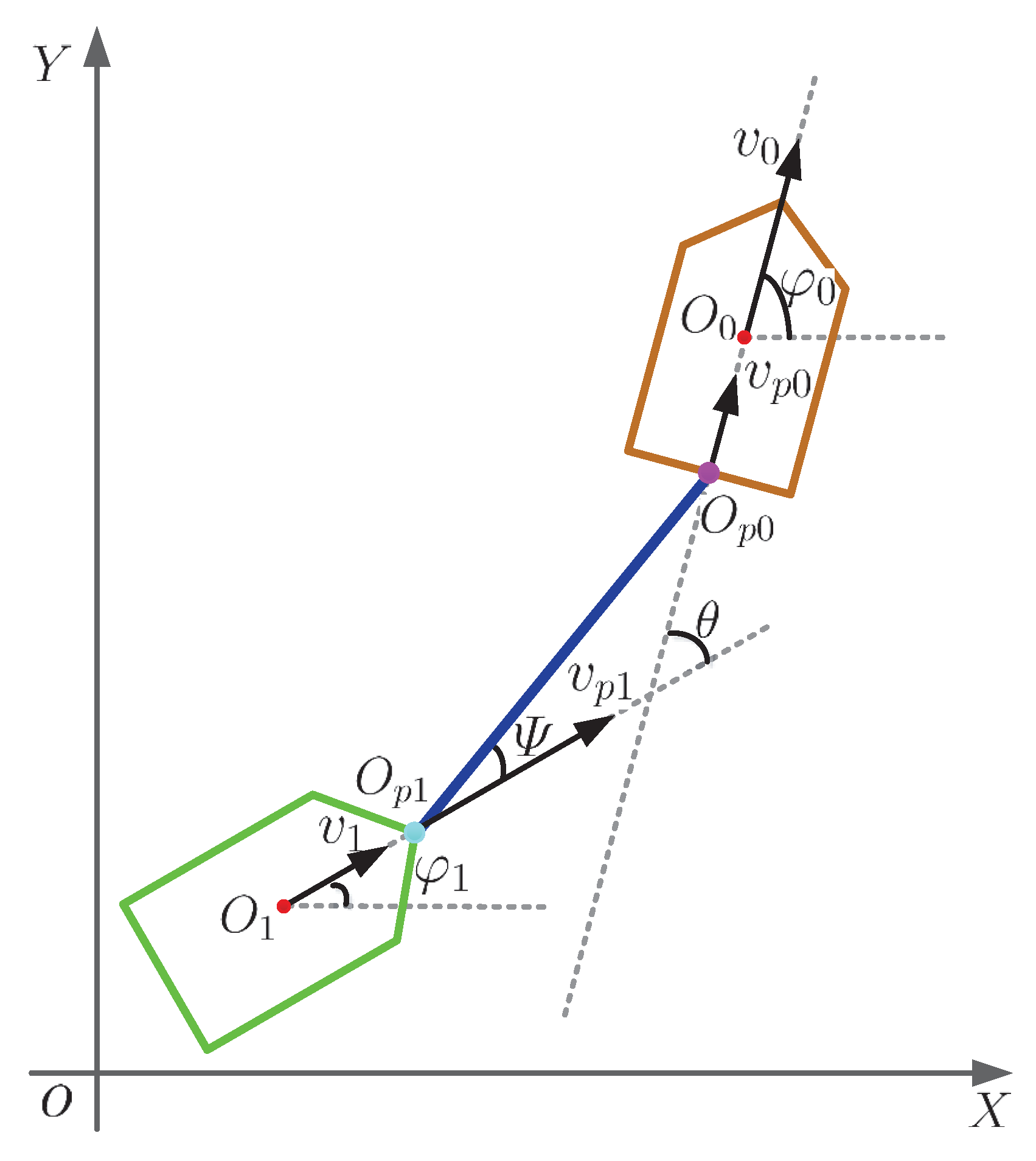
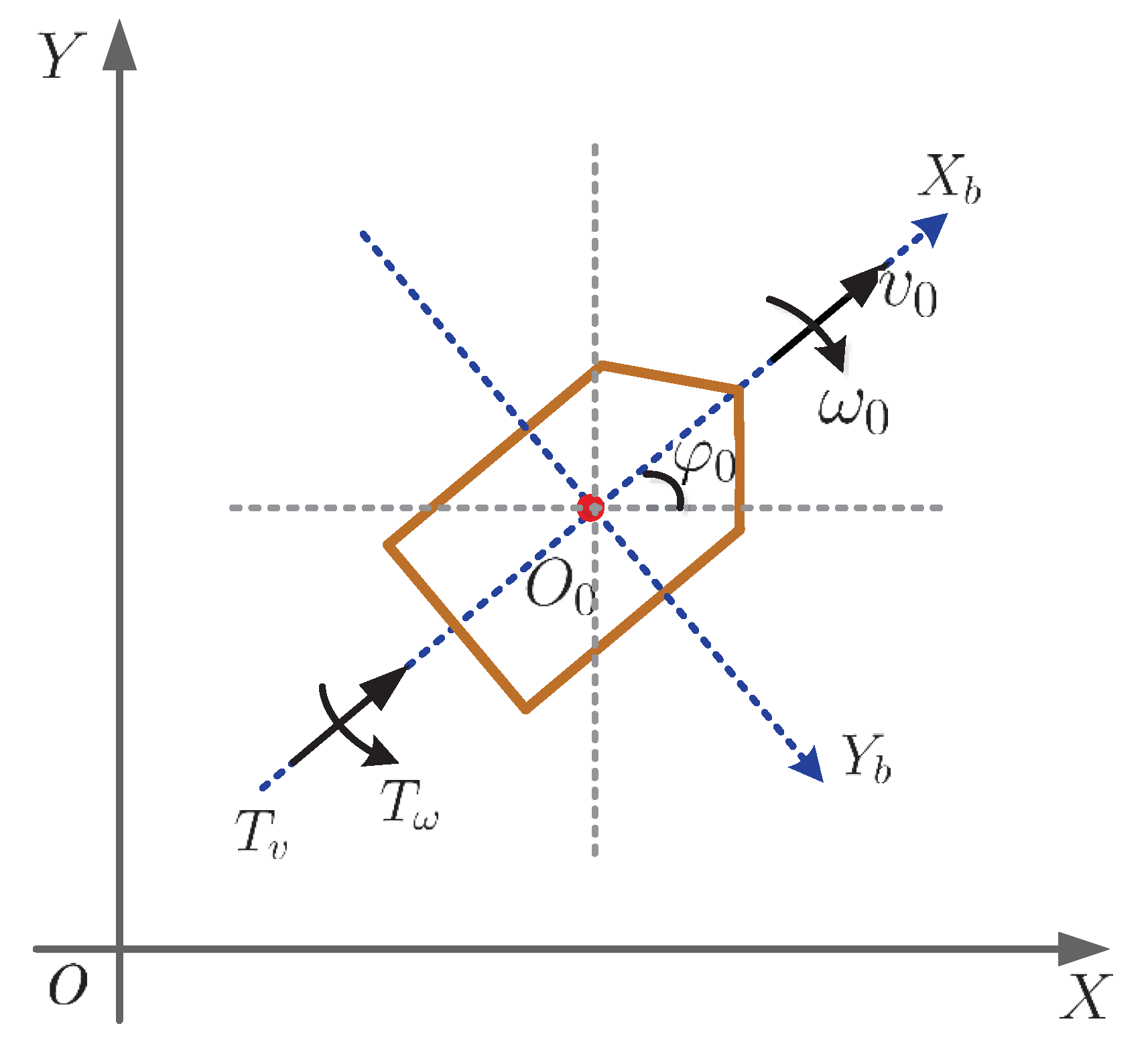
2.1. Kinematics Modeling

The generalized coordinate of the STS is defined as $\mathbf{p}={(x_0,y_0,{\phi }_0,\theta )}^{\mathrm{T}}$, and the system state is described by $(\mathbf{p},\dot{\mathbf{p}})$. Then, the motion states of other degrees of freedom can be deduced by its constraint equations.

For the STS, the motion of the tugboat and the towed ship is subject to the following nonholonomic constraints, respectively,

$$\left\{\begin{array}{c}-{\dot{x}}_0\sin {\phi }_0+{\dot{y}}_0\cos {\phi }_0=0,\hfill \\ v_0={\dot{x}}_0\cos {\phi }_0+{\dot{y}}_0\sin {\phi }_0,\hfill \end{array}\right.$$

(1)

and

$$\left\{\begin{array}{c}-{\dot{x}}_1\sin {\phi }_1+{\dot{y}}_1\cos {\phi }_1=0,\hfill \\ v_1={\dot{x}}_1\cos {\phi }_1+{\dot{y}}_1\sin {\phi }_1.\hfill \end{array}\right.$$

(2)

As shown in Figure 1, the speed relation between the tugboat and the towed ship is expressed as

$$\left\{\begin{array}{c}{v}_{p1}\cos \Psi =\cos (\theta -\Psi )v_{p0},\hfill \\ v_{p0}\sin (\theta -\Psi )+v_{p1}\sin \Psi =a(\dot{\Psi }-\dot{\theta }+{\dot{\phi }}_0).\hfill \end{array}\right.$$

(3)

Here, the first equation denotes that the velocity of joints $O_{p0}$ and $O_{p1}$ along the towline direction are equal. The second equation desribes the speed relation between the joints $O_{p0}$ and $O_{p1}$ in the vertical direction. Such speed relation causes coupling motion between the adjacent structures.

Substituting $\Psi =\mu \theta$ and the first equation of (3) into the second equation of (3), we obtain

$$\dot{\theta }=-\frac{\sin \theta }{a(1-\mu )\cos \Psi }{v}_{p0}+\frac{1}{1-\mu }{\dot{\phi }}_0.$$

(4)

Define $\Omega =\frac{\sin \theta }{\cos \Psi }$, and then (4) can be rewritten as

$$\dot{\theta }=-\frac{\Omega }{a(1-\mu )}{v}_{p0}+\frac{1}{1-\mu }{\dot{\phi }}_0.$$

(5)

Furthermore, according to the coordinates of point $O_0$ and $O_1$, we can get the positional coordinates of $O_{p0}(x_0-\frac{L}{2}\cos {\phi }_0,y_0-\frac{L}{2}\sin {\phi }_0)$ and $O_{p1}(x_1+\frac{L}{2}\cos {\phi }_1,y_1+\frac{L}{2}\sin {\phi }_1)$, where L is the length of the tugboat, as shown in Figure 1. In this way, the speed relations of points $O_{p0}$ and $O_0$, $O_{p1}$ and $O_1$ are expressed as

$$\left\{\begin{array}{c}{v}_{p0}^2={\dot{x}}_0^2+{\dot{y}}_0^2+\frac{L^2}{4}{\dot{\phi }}_0^2+L{\dot{\phi }}_0({\dot{x}}_0\sin {\phi }_0-{\dot{y}}_0\cos {\phi }_0),\hfill \\ v_{p1}^2={\dot{x}}_1^2+{\dot{y}}_1^2+\frac{L^2}{4}{\dot{\phi }}_1^2+L{\dot{\phi }}_1({\dot{y}}_1\cos {\phi }_1-{\dot{x}}_1\sin {\phi }_1).\hfill \end{array}\right.$$

(6)

Squaring both sides of the two equations of (1) and adding the two square equations, we obtain $v_0^2={\dot{x}}_0^2+{\dot{y}}_0^2$. Similarly, from (2), we have $v_1^2={\dot{x}}_1^2+{\dot{y}}_1^2$. In this way, (6) becomes

$$\left\{\begin{array}{c}{v}_{p0}^2=v_0^2+\frac{L^2}{4}{\dot{\phi }}_0^2,\hfill \\ v_{p1}^2=v_1^2+\frac{L^2}{4}{\dot{\phi }}_1^2=v_1^2+\frac{L^2}{4}{({\dot{\phi }}_0-\dot{\theta })}^2.\hfill \end{array}\right.$$

(7)

Substituting $v_{p0}$ and $v_{p1}$ of (7) into(3), one has

$$v_1=\sqrt{\frac{{\cos }^2(\theta -\Psi )}{{\cos }^2\Psi }(v_0^2+\frac{L^2}{4}{\dot{\phi }}_0^2)-\frac{L^2}{4}{({\dot{\phi }}_0-\dot{\theta })}^2}.$$

(8)

Then, substituting $v_{p0}$ of (7) into (5) gives

$$\dot{\theta }=-\frac{\Omega }{a(1-\mu )}\sqrt{v_0^2+\frac{L^2}{4}{\dot{\phi }}_0^2}+\frac{1}{(1-\mu )}{\dot{\phi }}_0.$$

(9)

With these preparations, all constraint equations of the STS are formulated by

$$\left\{\begin{array}{c}-{\dot{x}}_0\sin {\phi }_0+{\dot{y}}_0\cos {\phi }_0=0,\hfill \\ v_0={\dot{x}}_0\cos {\phi }_0+{\dot{y}}_0\sin {\phi }_0,\hfill \\ {\dot{\phi }}_0={\omega }_0,\hfill \\ \dot{\theta }=-\frac{\Omega }{a(1-\mu )}\sqrt{v_0^2+\frac{L^2}{4}{\dot{\phi }}_0^2}+\frac{1}{(1-\mu )}{\dot{\phi }}_0.\hfill \end{array}\right.$$

(10)

By using the motion laws derived from (10), the target trajectory curve can be transformed into a speed target of the tugboat [21], so that the dynamics equation of the STS can match the tracking target well. In fact, the towline is flexibly connected with the two ships. The angle between the rigid towline and the forward speed direction of the towed ship can be adjusted by a gear steering equipment. Then, according to the relationship of motion speed between the towed ship and the tugboat, the towed ship can move along the trajectory of the tugboat by choosing an appropriate steering angle coefficient $\mu$.

2.2. Dynamics Modeling of a Single Ship

In order to establish the dynamics model of the STS, we should first clarify the dynamics equation of a single ship, taking the single tugboat for example. As shown in Figure 2, an earthbound coordinate frame $O-XYZ$ is used to describe the motion of the single ship in the horizontal plane. The body-fixed coordinate frame $O_0-X_b{Y}_b{Z}_b$ centered at midship point $O_0$ of the single ship is used for better force analysis.

On the one hand, according to the kinematics equation in Reference [22] and neglecting the drifting speed, the dynamics equation of the tugboat is given by

$$\left\{\begin{array}{c}{x}_b=m_0{\dot{v}}_0,\hfill \\ z_b=I_{z0}{\dot{\omega }}_0,\hfill \end{array}\right.$$

(11)

where $x_b$ represents the component of the external force in the $X_b$ direction, and $z_b$ denotes the component of the external moment of inertia in the $Z_b$ direction.

On the other hand, according to force analysis of the hull [23], one has

$$\left\{\begin{array}{c}{x}_b=-M_{x0}{\dot{v}}_0-\frac{1}{2}\rho C_{f}S{v}_0^2+X_p+X_r,\hfill \\ z_b=-J_{z0}{\dot{\omega }}_0-\frac{1}{2}\rho L^{2}d{v}_0{\omega }_0(0.45\lambda -{\lambda }^2)(1+0.3\tau )+N_p+N_r,\hfill \end{array}\right.$$

(12)

where $X_p$ denotes the component force acting on the propeller along the $X_b$-axis, and $N_p$ represents the corresponding component of the inertia moment along the $Z_b$-axis. $X_r$ represents the component force on the rudder along the $X_b$-axis and $N_r$ is the corresponding component of the inertia moment along the $Z_b$-axis. $\rho$ is the water density. d is the full load draft height of the tugboat. S is the hull wet area of the tugboat. $\lambda$ is the aspect ratio of the rudder of the tugboat. $\tau$ is the trim value of the tugboat. And $C_f$ is the coefficient of frictional resistance.

It follows from (11) and (12) that the desired dynamics equation of the single tugboat is expressed by

$$\left\{\begin{array}{c}(m_0+M_{x0}){\dot{v}}_0=-\frac{1}{2}\rho C_{f}S{v}_0^2+X_p+X_r,\hfill \\ (I_{z0}+J_{z0}){\dot{\omega }}_0=-\frac{1}{2}\rho L^{2}d{v}_0{\omega }_0(0.45\lambda -{\lambda }^2)(1+0.3\tau )+N_p+N_r.\hfill \end{array}\right.$$

(13)

2.3. Dynamics Modeling

According to the dynamics Equation (13) of the single tugboat, the dynamics model of the STS can be presented by Reference [24]:

$$\left\{\begin{array}{c}(m_0+M_{x0}){\dot{v}}_0=-\frac{1}{2}\rho C_{f}S{v}_0^2+X_p+X_r-T\cos (\theta -\Psi ),\hfill \\ (I_{z0}+J_{z0}){\dot{\omega }}_0=-\frac{1}{2}\rho L^{2}d{v}_0{\omega }_0(0.45\lambda -{\lambda }^2)(1+0.3\tau )+N_p+N_r\hfill \\ -\frac{1}{2}TL\sin (\theta -\Psi ).\hfill \end{array}\right.$$

(14)

$$\left\{\begin{array}{c}(m_1+M_{x1}){\dot{v}}_1=-\frac{1}{2}\rho C_{f}S{v}_1^2+T\cos \Psi ,\hfill \\ (I_{z1}+J_{z1}){\dot{\omega }}_1=-\frac{1}{2}\rho L^{2}d{v}_1{\omega }_1(0.45\lambda -{\lambda }^2)(1+0.3\tau )+\frac{1}{2}TL\sin \Psi ,\hfill \end{array}\right.$$

(15)

where T is the towline tension. From (14), one has

$$\left\{\begin{array}{c}{\dot{v}}_0=\frac{-\frac{1}{2}\rho C_{f}S{v}_0^2+X_p+X_r-T\cos (\theta -\Psi )}{(m_0+M_{x0})},\hfill \\ {\dot{\omega }}_0=\frac{-\frac{1}{2}\rho L^{2}d{v}_0{\omega }_0(0.45\lambda -{\lambda }^2)(1+0.3\tau )+N_p+N_r-\frac{1}{2}TL\sin (\theta -\Psi )}{I_{z0}+J_{z0}}.\hfill \end{array}\right.$$

(16)

According to (15), the towline tension T is expressed as

$$\begin{array}{cc}\hfill T^2=& {[(m_1+M_{x1}){\dot{v}}_1+\frac{1}{2}\rho C_{f}S{v}_1^2]}^2+[\frac{2}{L}(I_{z1}+J_{z1}){\dot{\omega }}_1\hfill \\ \hfill & +\rho Ld{v}_1{\omega }_1(0.45\lambda -{\lambda }^2)(1+0.3\tau ){]}^2,\hfill \end{array}$$

(17)

where $v_1,{\phi }_1$ can be obtained according to (8), (9), and ${\omega }_1={\dot{\phi }}_1={\dot{\phi }}_0-\dot{\theta }$.

It follows from (16) and (17) that the dynamics equation of the STS is ultimately formulated as

$$\left\{\begin{array}{c}{\dot{v}}_0=\frac{-{\Delta }_2{v}_0^2+u_1}{{\Delta }_1},\hfill \\ {\dot{\omega }}_0=\frac{-{\Delta }_4{v}_0{\omega }_0+u_2}{{\Delta }_3},\hfill \end{array}\right.$$

(18)

where ${\Delta }_1=m_0+M_{x0}$, ${\Delta }_2=\frac{1}{2}\rho C_{f}S$, ${\Delta }_3=I_{z0}+J_{z0}$, ${\Delta }_4=\frac{1}{2}\rho L^{2}d(0.45\lambda -{\lambda }^2)(1+0.3\tau )$, $u_1=X_p+X_r-T\cos (\theta -\Psi )$, and $u_2=N_p+N_r-\frac{1}{2}TL\sin (\theta -\Psi )$.

3. Trajectory Tracking Control of the Ship Towing System

In order to make the tugboat track a given target trajectory curve accurately, the target trajectory curve should be firstly converted into a speed target form so as to match the dynamics equation. As such, the original motion task is converted into a general trajectory tracking control problem of the tugboat. Then, two torque controllers can be designed from the forward and yaw speed subsystems, to achieve the given trajectory tracking task.

3.1. Dynamical Tracking Target

In this subsection, we will solve the problem of converting the target curve to an appropriate speed tracking target so as to match the dynamics Equation (18). For a target trajectory curve $\tilde{\mathbf{r}}\left(t\right)={(\tilde{x}\left(t\right),\tilde{y}\left(t\right))}^{\mathrm{T}}$, the speed form of the target trajectory curve is expressed as [21]

$$\left\{\begin{array}{c}{\tilde{v}}_0=\sqrt{{\dot{\tilde{x}}}^2+{\dot{\tilde{y}}}^2},\hfill \\ {\tilde{\omega }}_0={\dot{\tilde{\phi }}}_0=\frac{\dot{\tilde{x}}\ddot{\tilde{y}}-\dot{\tilde{y}}\ddot{\tilde{x}}}{{\dot{\tilde{x}}}^2+{\dot{\tilde{y}}}^2}=k\left(t\right){\tilde{v}}_0,\hfill \end{array}\right.$$

(19)

where $k\left(t\right)=\frac{\dot{\tilde{x}}\ddot{\tilde{y}}-\dot{\tilde{y}}\ddot{\tilde{x}}}{{({\dot{\tilde{x}}}^2+{\dot{\tilde{y}}}^2)}^{\frac{3}{2}}}$ is the relative curvature of the target trajectory curve. We note that the relative curvature is the key point of the target trajectory curve. If the relative curvature is tracked very well, the tugboat can follow the target trajectory curve precisely. On this basis, the target trajectory curve $\tilde{\mathbf{r}}\left(t\right)$ can be further improved into a dynamical tracking target form as

$$\left\{\begin{array}{c}{\tilde{v}}_0=\dot{\varphi }\left(t\right),\hfill \\ {\tilde{\omega }}_0={\dot{\tilde{\phi }}}_0=k\left(s\left(t\right)\right)v_0,\hfill \end{array}\right.$$

(20)

where $v_0$ stands for the actual forward speed of the tugboat, and $\dot{\varphi }\left(t\right)$ represents an appropriate forward speed target which is given by

$$\dot{\varphi }\left(t\right)=l{\beta }^{2}t{\mathrm{e}}^{-\beta t}.$$

(21)

In (21), l is the length of the target curve, $\beta$ is an appropriate parameter according to actual needs [21].

It can be seen from (20) that the target trajectory curve can be converted into a speed target form with the relative curvature. Combined with the dynamics model, two torque controllers can be designed to implement the tracking task of the target trajectory curve. In fact, there are two main advantages by using the dynamical tracking target. First, by choosing an appropriate forward speed target, the initial speed error is equal to zero, which can significantly reduce the position error caused by the accumulated speeds errors. Second, the yaw rotation speed target depends on the actual forward speed, which can be adjusted from moment to moment. Moreover, no matter how large the actual forward speed error is, as long as the curvature tracking error is small enough, satisfactory tracking performance can still be achieved. As a consequence, the idea of dynamical tracking target can fundamentally solve the problem of accurate trajectory tracking.

3.2. Control Design

In this subsection, we will design two torque controllers $(u_1,u_2)$ for the dynamics Equation (18) by using the dynamical tracking target (20). We see that the yaw rotation speed target $\tilde{\omega }$ in the second equation of (20) is the product of the actual forward speed v and the relative curvature $k\left(s\right(t\left)\right)$. Therefore, the controller $u_1$ in the first equation of (18) should be firstly considered so as to obtain the actual forward speed.

3.2.1. Forward Speed Control Subsystem

At first, we consider the first equation of the dynamics model (18)

$${\dot{v}}_0=\frac{-{\Delta }_2{v}_0^2+u_1}{{\Delta }_1}.$$

(22)

Applying the feedback linearization method to (22) and letting

$$u_1={\Delta }_1{h}_1+{\Delta }_2{v}_0^2,$$

(23)

a simple control system is obtained as

$${\dot{v}}_0=h_1\left(t\right).$$

Defining ${\mathbf{X}}_1={(s_1,v_0)}^{\mathrm{T}}$ and $s_1={\int }_0^t{v}_0\left(\xi \right)\mathrm{d}\xi$, the forward speed subsystem is rewritten in a matrix form as

$${\dot{\mathbf{X}}}_1\left(t\right)={\mathbf{A}}_1{\mathbf{X}}_1\left(t\right)+{\mathbf{B}}_1{h}_1\left(t\right),$$

(24)

where ${\mathbf{A}}_1=\left[\begin{array}{cc}0& 1\\ 0& 0\end{array}\right]$, and ${\mathbf{B}}_1=\left[\begin{array}{c}0\\ 1\end{array}\right]$. In this way, (24) is transformed into an error system as

$$\dot{\mathbf{Y}}={\mathbf{A}}_1\mathbf{Y}+{\mathbf{B}}_1{h}_1\left(t\right)+\mathbf{\eta }\left(t\right),$$

(25)

where ${\tilde{\mathbf{X}}}_1={({\tilde{s}}_1,{\tilde{v}}_0)}^{\mathrm{T}},$${\tilde{s}}_1={\int }_0^t{\tilde{v}}_0\left(\tau \right)\mathrm{d}\tau$, $\mathbf{Y}={(y_1,y_2)}^{\mathrm{T}}={\mathbf{X}}_1-{\tilde{\mathbf{X}}}_1$, and $\mathbf{\eta }\left(t\right)={\mathbf{A}}_1{\tilde{\mathbf{X}}}_1-{\dot{\tilde{\mathbf{X}}}}_1.$ It is obvious that the integral of (21) with respect to t from 0 to infinity is convergent. Thus, a linear quadratic performance index is introduced as

$$J=\frac{1}{2}{\int }_0^{+\infty }[{\mathbf{Y}}^{\mathrm{T}}\left(t\right){\mathbf{Q}}_1\mathbf{Y}\left(t\right)+h_1^{\mathrm{T}}\left(t\right)\mathbf{R}{h}_1\left(t\right)]\mathrm{d}t.$$

Here, matrix ${\mathbf{Q}}_1$ should be large weight of the forward speed error. In this way, the forward speed error is able to be small enough by using optimal control. According to the linear quadratic optimal control theory, the optimal control of forward speed error subsystem (25) is formulated as

$$h_1\left(t\right)=-{\mathbf{R}}^{-1}{\mathbf{B}}_1^{\mathrm{T}}[\mathbf{P}\mathbf{Y}+\mathbf{b}\left(t\right)].$$

(26)

where $\mathbf{P}\in {\mathbb{R}}^{2\times 2}$ and $\mathbf{b}\left(t\right)\in {\mathbb{R}}^2$ satisfy the following equations, respectively,

$$\left\{\begin{array}{c}-{\mathbf{PA}}_1-{\mathbf{A}}_1^{\mathrm{T}}\mathbf{P}+\mathbf{P}{\mathbf{B}}_1{\mathbf{R}}^{-1}{\mathbf{B}}_1^{\mathrm{T}}\mathbf{P}-{\mathbf{Q}}_1=\mathbf{0},\hfill \\ \dot{\mathbf{b}}=-{[{\mathbf{A}}_1-{\mathbf{B}}_1{\mathbf{R}}^{-1}{\mathbf{B}}_1^{\mathrm{T}}\mathbf{P}]}^{\mathrm{T}}\mathbf{b}-\mathbf{P}\mathbf{\eta }\left(t\right),\mathbf{b}(+\infty )=\mathbf{0}.\hfill \end{array}\right.$$

Substituting (26) into (23), the controller $u_1$ is formulated by

$$u_1=-{\Delta }_1{\mathbf{R}}^{-1}{\mathbf{B}}_1^{\mathrm{T}}[\mathbf{P}\mathbf{Y}+\mathbf{b}\left(t\right)]+{\Delta }_2{v}_0^2.$$

3.2.2. Yaw Rotation Speed Control Subsystem

Since the actual forward speed v is obtained, we now consider the yaw rotation speed subsystem in the second equation of (18). First, the state equation of the reference model is obtained as

$${\Delta }_3{\dot{\omega }}_0+{\Delta }_4{v}_0{\omega }_0={\mathbf{Y}}_{21}{\mathbf{D}}_2{\mathbf{Y}}_{22}=u_2,$$

(27)

where ${\mathbf{D}}_2=\mathrm{diag}({\Delta }_3,{\Delta }_4),$ ${\mathbf{Y}}_{21}=({\dot{\omega }}_0,1)$, and ${\mathbf{Y}}_{22}={(1,{\omega }_0{v}_0)}^{\mathrm{T}}.$ Since (27) is strongly nonlinear, it is unlikely to obtain an exact solution. Therefore, to seek an approximate solution, we introduce the adaptive control method based on its inverse dynamics. To this end, the basic part of controller $u_2$ is designed as

$$u_{20}={\widehat{\Delta }}_3{s}_2+{\widehat{\Delta }}_4{v}_0{\omega }_0,$$

(28)

which yields the adjusted system of (27) as follows:

$${\Delta }_3{\dot{\omega }}_0+{\Delta }_4{v}_0{\omega }_0=u_{20}.$$

(29)

Here, $s_2={\dot{\tilde{\omega }}}_0-k_2({\omega }_0-{\tilde{\omega }}_0)$ is the adaptation law, ${\tilde{\omega }}_0$ is the ideal yaw rotation speed target of the tugboat, $k_2$ is an adjustable control parameter, $e_2={\omega }_0-{\tilde{\omega }}_0$ is the yaw rotation speed error, and ${\widehat{\Delta }}_3,{\widehat{\Delta }}_4$ are the estimated values of ${\Delta }_3,{\Delta }_4$, respectively. Besides, ${\widehat{\mathbf{D}}}_2=\mathrm{diag}({\widehat{\Delta }}_3,{\widehat{\Delta }}_4)$ is defined as the estimated value of ${\mathbf{D}}_2$. The adjustment gain coefficient $k_2$ can be obtained by using Lyapunov stability theory, thereby getting the adaptation law $s_2$. It can be seen from (28) and (29) that large errors between ${\widehat{\Delta }}_3$ and ${\Delta }_3$, ${\widehat{\Delta }}_4$ and ${\Delta }_4$ may deteriorate the tracking performance, which can be overcome by adjusting the adjustable control parameter $k_2$. Substituting (28) into (29), one has

$${\widehat{\Delta }}_3({\dot{\tilde{\omega }}}_0-k_2({\omega }_0-{\tilde{\omega }}_0))+{\widehat{\Delta }}_4{v}_0{\omega }_0={\Delta }_3{\dot{\omega }}_0+{\Delta }_4{v}_0{\omega }_0,$$

which yields

$$-{\widehat{\Delta }}_3({\dot{\omega }}_0-{\dot{\tilde{\omega }}}_0+k_2({\omega }_0-{\tilde{\omega }}_0))+({\widehat{\Delta }}_3-{\Delta }_3){\dot{\omega }}_0+({\widehat{\Delta }}_4-{\Delta }_4)v_0{\omega }_0=0.$$

(30)

It follows from (30) and ${\dot{e}}_2={\dot{\omega }}_0-{\dot{\tilde{\omega }}}_0$ that

$${\widehat{\Delta }}_3({\dot{e}}_2+k_2{e}_2)={\Delta }_{3e}{\dot{\omega }}_0+{\Delta }_{4e}{v}_0{\omega }_0,$$

(31)

where ${\Delta }_{3e}={\widehat{\Delta }}_3-{\Delta }_3$, ${\Delta }_{4e}={\widehat{\Delta }}_4-{\Delta }_4$, and ${\mathbf{D}}_{2e}={\widehat{\mathbf{D}}}_2-{\mathbf{D}}_2$. Then, together with (27), one has

$${\Delta }_{3e}{\dot{\omega }}_0+{\Delta }_{4e}{v}_0{\omega }_0={\mathbf{Y}}_{21}{\mathbf{D}}_{2e}{\mathbf{Y}}_{22}.$$

(32)

Assume that ${\widehat{\Delta }}_3$ is reversible, and then (31) can be written as

$$({\dot{e}}_2+k_2{e}_2)={\widehat{\Delta }}_3^{-1}({\Delta }_{3e}{\dot{\omega }}_0+{\Delta }_{4e}{v}_0{\omega }_0).$$

Combining (32), one has

$${\dot{e}}_2+k_2{e}_2={\widehat{\Delta }}_3^{-1}{\mathbf{Y}}_{21}{\mathbf{D}}_{2e}{\mathbf{Y}}_{22},$$

(33)

which is the error state equation of (27). Furthermore, (33) can be rewritten in a state equation form as

$${\dot{\mathbf{X}}}_2={\mathbf{A}}_2{\mathbf{X}}_2+{\mathbf{B}}_2{\widehat{\Delta }}_3^{-1}{\mathbf{Y}}_{21}{\mathbf{D}}_{2e}{\mathbf{Y}}_{22},$$

(34)

where ${\mathbf{A}}_2=\left(\begin{array}{cc}0& 1\\ 0& -k_2\end{array}\right)$, ${\mathbf{B}}_2=\left(\begin{array}{c}0\\ 1\end{array}\right)$ and ${\mathbf{X}}_2=\left(\begin{array}{c}{\zeta }_2\\ e_2\end{array}\right)$ with ${\zeta }_2={\int }_0^t{e}_2\left(\tau \right)\mathrm{d}\tau$.

On the other hand, to improve the precision of the estimated matrix ${\widehat{\mathbf{D}}}_2$, a symmetric matrix ${\mathbf{Q}}_2$ is chosen to satisfy the following Lyapunov equation:

$${\mathbf{A}}_2^{\mathrm{T}}{\mathbf{D}}_2+{\mathbf{D}}_2{\mathbf{A}}_2+{\mathbf{Q}}_2=\mathbf{0},$$

(35)

which can be rewritten in a more detailed form as

$$\begin{array}{cc}\hfill \left(\begin{array}{cc}0& 0\\ 1& -k_2\end{array}\right)\left(\begin{array}{cc}{\Delta }_3& 0\\ 0& {\Delta }_4\end{array}\right)+\left(\begin{array}{cc}{\Delta }_3& 0\\ 0& {\Delta }_4\end{array}\right)\left(\begin{array}{cc}0& 1\\ 0& -k_2\end{array}\right)=& \left(\begin{array}{cc}0& {\Delta }_3\\ {\Delta }_3& -2k_2{\Delta }_4\end{array}\right)\hfill \\ \hfill =& \left(\begin{array}{cc}-{\mathbf{Q}}_{11}& -{\mathbf{Q}}_{12}\\ -{\mathbf{Q}}_{21}& -{\mathbf{Q}}_{22}\end{array}\right),\hfill \end{array}$$

(36)

where ${\mathbf{Q}}_2=\left(\begin{array}{cc}{\mathbf{Q}}_{11}& {\mathbf{Q}}_{12}\\ {\mathbf{Q}}_{21}& {\mathbf{Q}}_{22}\end{array}\right)$. It follows from (36) that

$$\left\{\begin{array}{c}{\mathbf{Q}}_{11}=0,\hfill \\ {\mathbf{Q}}_{12}={\mathbf{Q}}_{21}=-{\Delta }_3,\hfill \\ {\mathbf{Q}}_{22}=2k_2{\Delta }_4.\hfill \end{array}\right.$$

Therefore, we can uniquely determine the positive definite matrix ${\mathbf{D}}_2$ by selecting an appropriate matrix ${\mathbf{Q}}_2$.

After that, apositive definite quadratic function is defined as

$$V={\mathbf{X}}_2^{\mathrm{T}}{\mathbf{D}}_2{\mathbf{X}}_2+{\mathbf{Y}}_{22}^{\mathrm{T}}{\mathbf{D}}_{2e}^{\mathrm{T}}{\Gamma }_2{\mathbf{D}}_{2e}{\mathbf{Y}}_{22},$$

(37)

where ${\mathbf{D}}_2$ is the unique positive definite solution of (34), and ${\Gamma }_2$ is an appropriate positive definite symmetric matrix. Differentiating both sides of (35) with respect to t and combining (34) with (35), one has

$$\begin{array}{cc}\hfill \dot{V}=& {\dot{\mathbf{X}}}_2^{\mathrm{T}}{\mathbf{D}}_2{\mathbf{X}}_2+{\mathbf{X}}_2^{\mathrm{T}}{\mathbf{D}}_2{\dot{\mathbf{X}}}_2+{\dot{\mathbf{Y}}}_{22}^{\mathrm{T}}{\mathbf{D}}_{2e}^{\mathrm{T}}{\Gamma }_2{\mathbf{D}}_{2e}{\mathbf{Y}}_{22}+{\mathbf{Y}}_{22}^{\mathrm{T}}{\dot{\mathbf{D}}}_{2e}^{\mathrm{T}}{\Gamma }_2{\mathbf{D}}_{2e}{\mathbf{Y}}_{22}\hfill \\ \hfill & +{\mathbf{Y}}_{22}^{\mathrm{T}}{\mathbf{D}}_{2e}^{\mathrm{T}}{\Gamma }_2{\dot{\mathbf{D}}}_{2e}{\mathbf{Y}}_{22}+{\mathbf{Y}}_{22}^{\mathrm{T}}{\mathbf{D}}_{2e}^{\mathrm{T}}{\Gamma }_2{\mathbf{D}}_{2e}{\dot{\mathbf{Y}}}_{22}\hfill \\ \hfill =& {({\mathbf{A}}_2{\mathbf{X}}_2+{\mathbf{B}}_2{\widehat{\Delta }}_3^{-1}{\mathbf{Y}}_{21}{\mathbf{D}}_{2e}{\mathbf{Y}}_{22})}^{\mathrm{T}}{\mathbf{D}}_2{\mathbf{X}}_2+{\mathbf{X}}_2^{\mathrm{T}}{\mathbf{D}}_2({\mathbf{A}}_2{\mathbf{X}}_2+{\mathbf{B}}_2{\widehat{\Delta }}_3^{-1}{\mathbf{Y}}_{21}{\mathbf{D}}_{2e}{\mathbf{Y}}_{22})\hfill \\ \hfill & +{\dot{\mathbf{Y}}}_{22}^{\mathrm{T}}{\mathbf{D}}_{2e}^{\mathrm{T}}{\Gamma }_2{\mathbf{D}}_{2e}{\mathbf{Y}}_{22}+{\mathbf{Y}}_{22}^{\mathrm{T}}{\dot{\mathbf{D}}}_{2e}^{\mathrm{T}}{\Gamma }_2{\mathbf{D}}_{2e}{\mathbf{Y}}_{22}+{\mathbf{Y}}_{22}^{\mathrm{T}}{\mathbf{D}}_{2e}^{\mathrm{T}}{\Gamma }_2{\dot{\mathbf{D}}}_{2e}{\mathbf{Y}}_{22}+{\mathbf{Y}}_{22}^{\mathrm{T}}{\mathbf{D}}_{2e}^{\mathrm{T}}{\Gamma }_2{\mathbf{D}}_{2e}{\dot{\mathbf{Y}}}_{22}\hfill \\ \hfill =& {\mathbf{X}}_2^{\mathrm{T}}{\mathbf{A}}_2^{\mathrm{T}}{\mathbf{D}}_2{\mathbf{X}}_2+{\widehat{\Delta }}_3^{-1}{\mathbf{Y}}_{22}^{\mathrm{T}}{\mathbf{D}}_{2e}^{\mathrm{T}}{\mathbf{Y}}_{21}^{\mathrm{T}}{\mathbf{B}}_2^{\mathrm{T}}{\mathbf{D}}_2{\mathbf{X}}_2+{\mathbf{X}}_2^{\mathrm{T}}{\mathbf{D}}_2({\mathbf{A}}_2{\mathbf{X}}_2+{\mathbf{B}}_2{\widehat{\Delta }}_3^{-1}{\mathbf{Y}}_{21}{\mathbf{D}}_{2e}{\mathbf{Y}}_{22})\hfill \\ \hfill & +{\dot{\mathbf{Y}}}_{22}^{\mathrm{T}}{\mathbf{D}}_{2e}^{\mathrm{T}}{\Gamma }_2{\mathbf{D}}_{2e}{\mathbf{Y}}_{22}+{\mathbf{Y}}_{22}^{\mathrm{T}}{\dot{\mathbf{D}}}_{2e}^{\mathrm{T}}{\Gamma }_2{\mathbf{D}}_{2e}{\mathbf{Y}}_{22}+{\mathbf{Y}}_{22}^{\mathrm{T}}{\mathbf{D}}_{2e}^{\mathrm{T}}{\Gamma }_2{\dot{\mathbf{D}}}_{2e}{\mathbf{Y}}_{22}+{\mathbf{Y}}_{22}^{\mathrm{T}}{\mathbf{D}}_{2e}^{\mathrm{T}}{\Gamma }_2{\mathbf{D}}_{2e}{\dot{\mathbf{Y}}}_{22}\hfill \\ \hfill =& {\mathbf{X}}_2^{\mathrm{T}}(-{\mathbf{Q}}_2-{\mathbf{D}}_2{\mathbf{A}}_2){\mathbf{X}}_2+{\widehat{\Delta }}_3^{-1}{\mathbf{Y}}_{22}^{\mathrm{T}}{\mathbf{D}}_{2e}^{\mathrm{T}}{\mathbf{Y}}_{21}^{\mathrm{T}}{\mathbf{B}}_2^{\mathrm{T}}{\mathbf{D}}_2{\mathbf{X}}_2+{\mathbf{X}}_2^{\mathrm{T}}{\mathbf{D}}_2({\mathbf{A}}_2{\mathbf{X}}_2+{\mathbf{B}}_2{\widehat{\Delta }}_3^{-1}{\mathbf{Y}}_{21}{\mathbf{D}}_{2e}{\mathbf{Y}}_{22})\hfill \\ \hfill & +{\dot{\mathbf{Y}}}_{22}^{\mathrm{T}}{\mathbf{D}}_{2e}^{\mathrm{T}}{\Gamma }_2{\mathbf{D}}_{2e}{\mathbf{Y}}_{22}+{\mathbf{Y}}_{22}^{\mathrm{T}}{\dot{\mathbf{D}}}_{2e}^{\mathrm{T}}{\Gamma }_2{\mathbf{D}}_{2e}{\mathbf{Y}}_{22}+{\mathbf{Y}}_{22}^{\mathrm{T}}{\mathbf{D}}_{2e}^{\mathrm{T}}{\Gamma }_2{\dot{\mathbf{D}}}_{2e}{\mathbf{Y}}_{22}+{\mathbf{Y}}_{22}^{\mathrm{T}}{\mathbf{D}}_{2e}^{\mathrm{T}}{\Gamma }_2{\mathbf{D}}_{2e}{\dot{\mathbf{Y}}}_{22}\hfill \\ \hfill =& -{\mathbf{X}}_2^{\mathrm{T}}{\mathbf{Q}}_2{\mathbf{X}}_2+2{\mathbf{Y}}_{22}^{\mathrm{T}}{\mathbf{D}}_{2e}^{\mathrm{T}}{\mathbf{Y}}_{21}^{\mathrm{T}}{\widehat{\Delta }}_3^{-1}{\mathbf{B}}_2^{\mathrm{T}}{\mathbf{D}}_2{\mathbf{X}}_2+2{\mathbf{Y}}_{22}^{\mathrm{T}}{\mathbf{D}}_{2e}^{\mathrm{T}}{\Gamma }_2{\dot{\mathbf{D}}}_{2e}{\mathbf{Y}}_{22}+2{\mathbf{Y}}_{22}^{\mathrm{T}}{\mathbf{D}}_{2e}^{\mathrm{T}}{\Gamma }_2{\mathbf{D}}_{2e}{\dot{\mathbf{Y}}}_{22}\hfill \\ \hfill =& -{\mathbf{X}}_2^{\mathrm{T}}{\mathbf{Q}}_2{\mathbf{X}}_2+2{\mathbf{Y}}_{22}^{\mathrm{T}}{\mathbf{D}}_{2e}^{\mathrm{T}}[{\mathbf{Y}}_{21}^{\mathrm{T}}{\widehat{\Delta }}_3^{-1}{\mathbf{B}}_2^{\mathrm{T}}{\mathbf{D}}_2{\mathbf{X}}_2+{\Gamma }_2{\dot{\mathbf{D}}}_{2e}{\mathbf{Y}}_{22}+{\Gamma }_2{\mathbf{D}}_{2e}{\dot{\mathbf{Y}}}_{22}].\hfill \end{array}$$

(38)

Since ${\dot{\mathbf{D}}}_{2e}={\dot{\widehat{\mathbf{D}}}}_2$, ${\widehat{\mathbf{D}}}_2$ is assumed to

$${\dot{\widehat{\mathbf{D}}}}_2=-{\Gamma }_2^{-1}({\mathbf{Y}}_{21}^{\mathrm{T}}{\widehat{\Delta }}_3^{-1}{\mathbf{B}}_2^{\mathrm{T}}{\mathbf{D}}_2{\mathbf{X}}_2+{\Gamma }_2{\mathbf{D}}_{2e}{\dot{\mathbf{Y}}}_{22}){\mathbf{Y}}_{22}^{-1}.$$

(39)

If follows from (38) and (39) that

$$\dot{V}=-{\mathbf{X}}_2^{\mathrm{T}}{\mathbf{Q}}_2{\mathbf{X}}_2\le 0.$$

(40)

We have seen, from (37) and (40), that (33) is stablized. In this way, the adaptive control $u_{20}$ can track the ideal yaw rotation speed ${\tilde{\omega }}_0$ well, which ensures that all signals of the control system are bounded. Thus, by choosing appropriate parameters, the tracking error of the yaw speed can be controlled in a small area.

In order to improve the robustness of the yaw rotation speed subsystem, we introduce an integral sliding mode control method. On the one hand, the basic part of controller $u_2$ is designed as (28). On the other hand, a sliding mode function $S\left(\omega \right(t\left)\right)$ is defined as [25]

$$S\left(\omega \left(t\right)\right)=G[\omega \left(t\right)-{\omega }_0\left(0\right)]-G{\int }_0^t{\dot{\tilde{\omega }}}_0\left(\eta \right)\mathrm{d}\eta ,$$

where G is an appropriate constant. Then, the switching control part is designed on the integral sliding mainifold which is defined as

$$S\left({\omega }_0\left(t\right)\right)=0.$$

Thus, the switching control part of controller $u_2$ is designed as

$$u_{21}=-(G^{-1}\gamma +\epsilon \Vert e_2\Vert )\mathrm{sgn}\left(S\left({\omega }_0\left(t\right)\right)\right).$$

(41)

where $\epsilon$ is the control parameter related to the uncertainties, and $\gamma$ is the sliding mode control parameter. As a consequence, from (28) and (41), the controller is eventually designed as

$$u_2=u_{20}+u_{21}.$$

4. Simulation Results

In this section, we present three simulation results to verify the effectiveness of the proposed method. First, we performed a comparison between using the dynamical target and the statical target. Then, we report the actual trajectories of the towed ship affected by different steering coefficients. Finally, we give an uncertain factor acted on the forward speed subsystem to validate the robustness of the proposed controller.

The target trajectory curve of the STS is assumed to be

$$\begin{array}{c}\hfill {\tilde{\mathbf{r}}}_0={({\tilde{x}}_0\left(t\right),{\tilde{y}}_0\left(t\right))}^{\mathrm{T}}={(80sin\left(\frac{t-\pi }{2}\right)+40t-40\pi ,80-80cos\left(\frac{t-\pi }{2}\right))}^{\mathrm{T}},\end{array}$$

where $t\in [0,2\pi ],l=80\sqrt{2},\dot{\varphi }\left(t\right)=80\sqrt{2}t{e}^{-t},k_0\left(s\left(t\right)\right)=\frac{1}{320cos\left(\frac{t-\pi }{4}\right)}$.

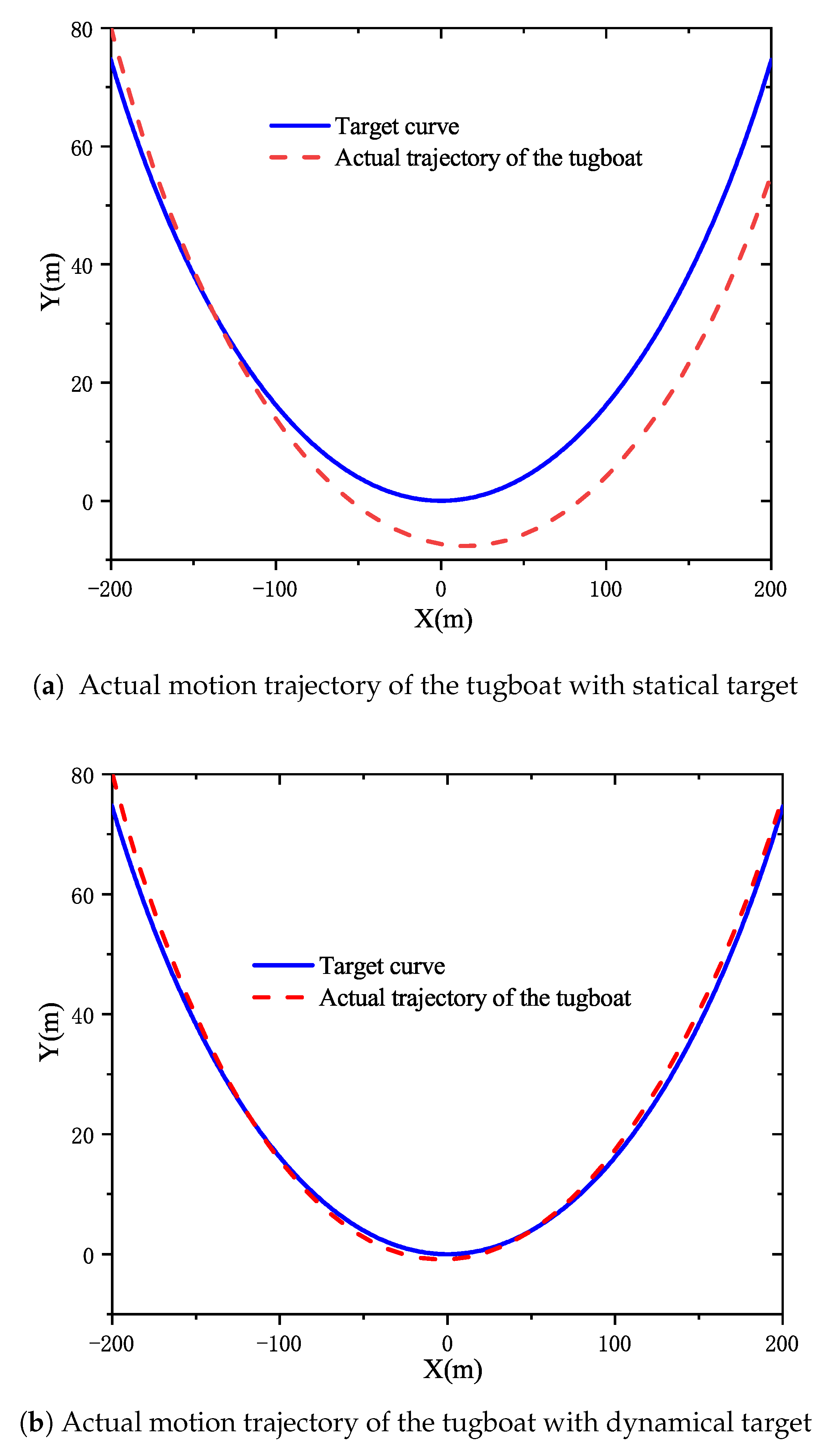
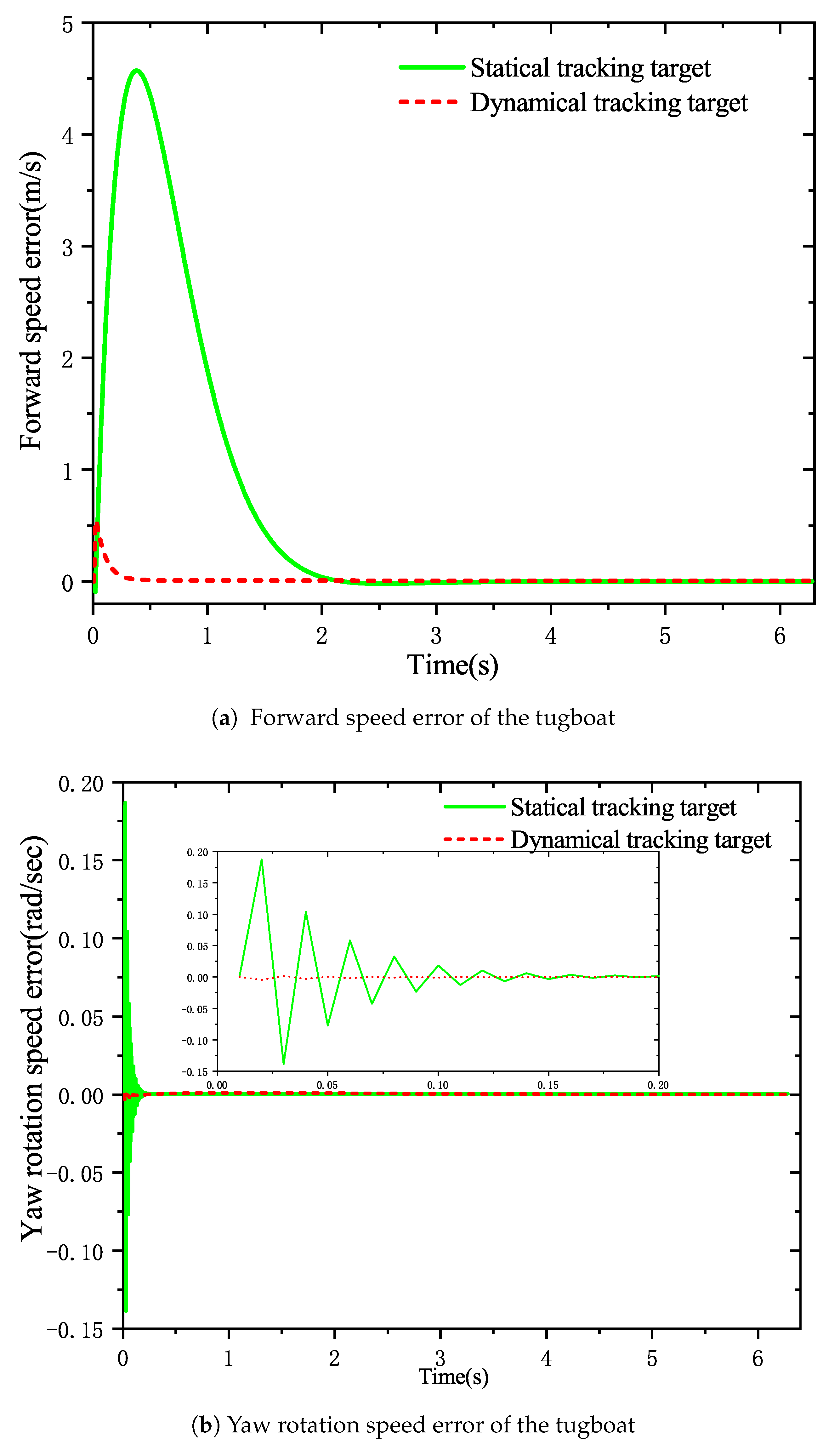
4.1. A Comparison between the Dynamical Target and Statical Target

On the one hand, the statical tracking target (19) is expressed by

$$\left\{\begin{array}{c}{\tilde{v}}_0=\sqrt{{\dot{\tilde{x}}}^2+{\dot{\tilde{y}}}^2}=80cos\left(\frac{t-\pi }{4}\right),\hfill \\ {\tilde{\omega }}_0=\frac{\dot{\tilde{x}}\ddot{\tilde{y}}-\ddot{\tilde{x}}\dot{\tilde{y}}}{{\dot{\tilde{x}}}^2+{\dot{\tilde{y}}}^2}=\frac{1}{4}.\hfill \end{array}\right.$$

(42)

If we use the statical tracking target (42) to design controller $u_1$ and $u_2$, the initial speed error is not zero, given by

$$\left\{\begin{array}{c}{v}_0\left(0\right)-{\tilde{v}}_0\left(0\right)=-80cos(-\frac{\pi }{4})=-40\sqrt{2},\hfill \\ {\omega }_0\left(0\right)-{\tilde{\omega }}_0\left(0\right)=-\frac{1}{4}.\hfill \end{array}\right.$$

On the other hand, the dynamical tracking target (20) is expressed by

$$\left\{\begin{array}{c}{\tilde{v}}_0=80\sqrt{2}t{e}^{-t},\hfill \\ {\tilde{\omega }}_0=k_0\left(s\right)v_0\left(t\right).\hfill \end{array}\right.$$

The relative parameters of the towing system are set as $\lambda =1.3,L=2.6\mathrm{m},\tau =0.25,S=3.3{\mathrm{m}}^2,\rho =1000\mathrm{kg}/{\mathrm{m}}^3,d=0.1\mathrm{m},C_f=0.063,m_0+M_{x0}=103\mathrm{kg},m_1+M_{x1}=103\mathrm{kg},$$I_{z0}+J_{z0}=30\mathrm{kg}·{\mathrm{m}}^2,I_{z1}+J_{z1}=30\mathrm{kg}·{\mathrm{m}}^2,Q_1=\mathrm{diag}(10,100),R=1,k_2=204,G=1,\epsilon =0.1,\gamma =0.3.$ Therefore, all the required quantities in the trajectory tracking controllers $u_1$ and $u_2$ are available in hand. Accordingly, the time histories of all state variables can be simulated.

As can be seen in Figure 3, by using the dynamical tracking target, both the initial forward speed and yaw rotation speed errors are smaller than the one using statical tracking target. Comparing Figure 4a with Figure 4b, we see that the actual motion trajectory of the tugboat deviates largely from the target curve by using the statical tracking target, whereas the actual motion trajectory of the tugboat coincides well the target curve via the dynamical tracking target. In other words, by using the dynamical tracking target, accurate trajectory tracking can be achieved as long as the curvature tracking error is controllable. Even though forward speed and yaw rotation speed errors are large, accurate tracking can be also maintained as long as the relative curvature is well tracked.

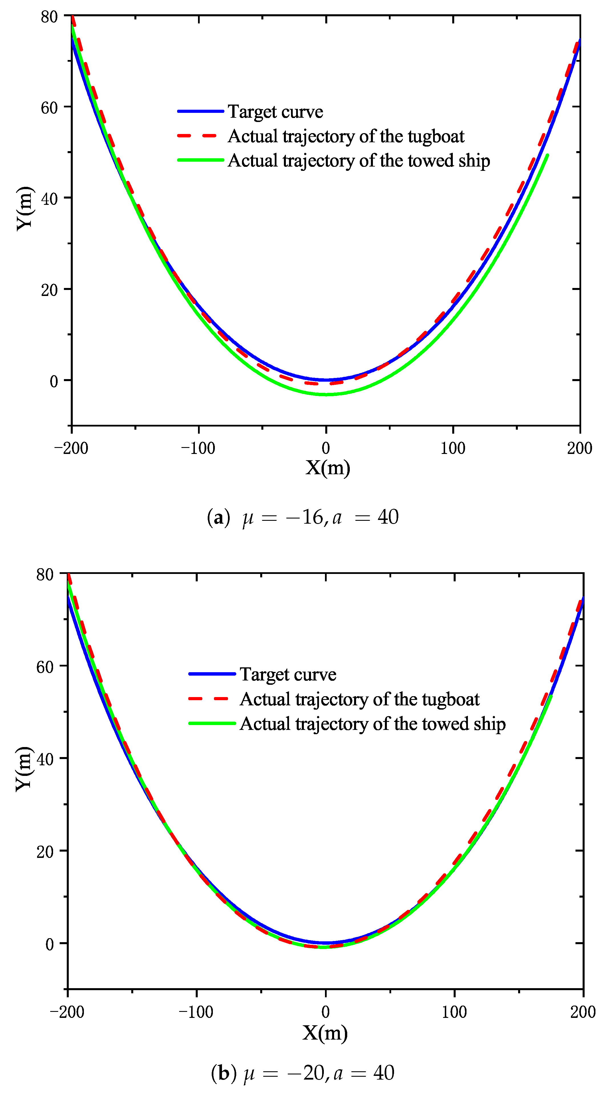
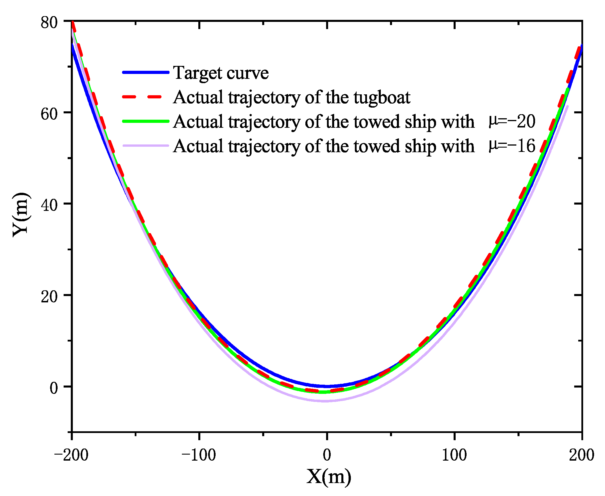
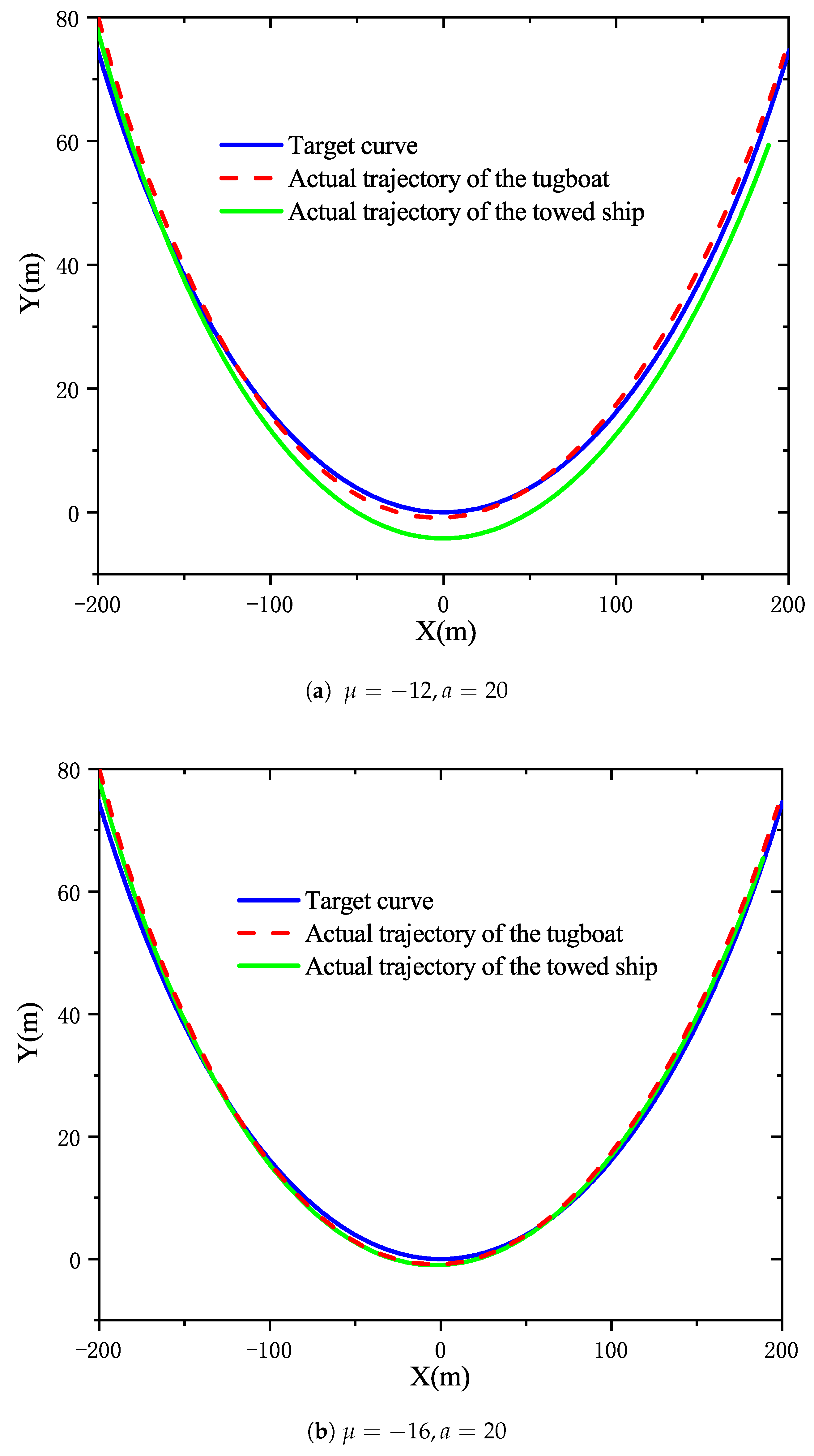
4.2. Actual Trajectories of the Towed Ship with Different Steering Coefficients

In order to further investigate the influence of the steering coefficient on the actual trajectory of the towed ship, we choose different steering coefficients and lengths of towline for simulations.

When the length of towline is relatively small, such as $a=20\mathrm{m}$, the actual motion trajectory of the towed ship deviates largely from the target curve, if the steering coefficient $\mu =-12$ is adopted, as depicted in Figure 5a. However, for the same length of the towline, the actual trajectory of the towed ship follows very well with the target curve by using the steering coefficient $\mu =-16$ in Figure 5b. When the length of the towline is relatively large, such as $a=40\mathrm{m}$, we need a larger steering coefficient to obtain a satisfactory tracking performance, such as $\mu =-20$, as depicted in Figure 6. As a consequence, when the length of the towline is smaller, a satisfactory trajectory tracking performance can be obtained with smaller steering coefficient, whereas, when the length of the towline is large, a larger steering coefficient must be applied to keep the tracking error of the towed ship within a smaller range.

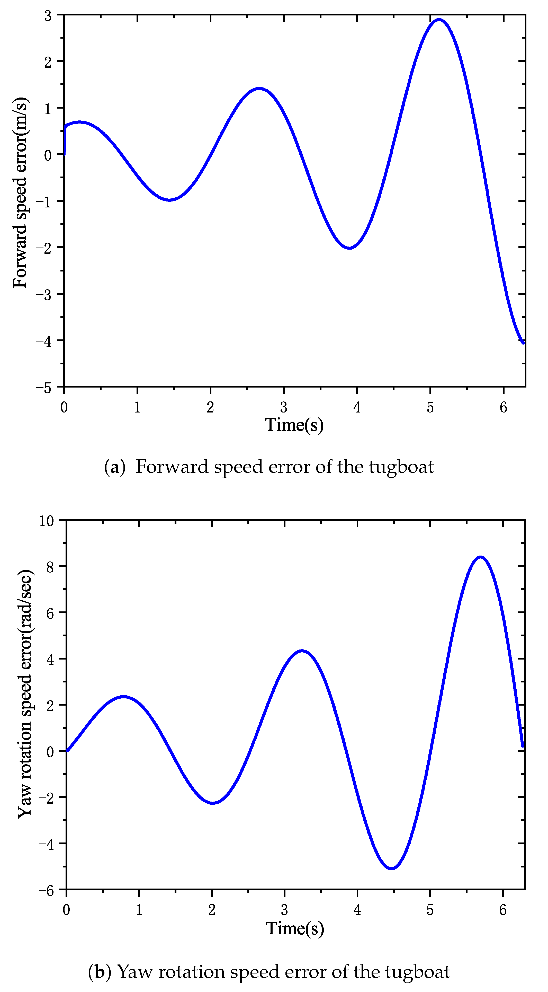
4.3. Robustness of the Proposed Controller

Since the controllers are designed by considering the sliding mode control and inverse dynamics adaptive control methods simultaneously, it has highly robust. Moreover, by using the dynamical tracking target, even though the forward speed and yaw rotation speed error subsystems are unstable due to uncertain factors, the towed ship is also able to achieve satisfactory tracking performance.

Assume that the forward speed error subsystem is subject to an uncertain factor, which is given by

$$\dot{\mathbf{Y}}={\mathbf{A}}_1\mathbf{Y}+{\mathbf{B}}_1{u}_1\left(t\right)+\mathbf{\eta }\left(t\right)+\mathit{d}\left(t\right),$$

where $\mathit{d}\left(t\right)={(10.2y_1,10.2y_2)}^{\mathrm{T}}$ is an uncertain factor.

As shown in Figure 7 and Figure 8, although forward speed and yaw rotation speed errors are large and even divergent, the actual motion trajectory of the tugboat almost coincides with the target curve. The main reason is that the relative curvature error which is obtained by dividing the actual yaw rotation speed by the actual forward speed is small via the dynamical tracking target. Therefore, as long as the relative curvature error is small enough, the accurate tracking of the target trajectory curve can still be guaranteed. Moreover, the towed ship can also obtain satisfactory tracking performance by means of an appropriate steering coefficient, such as $\mu =-20$. Otherwise, there will be a large deviation from the target trajectory curve, such as $\mu =-16$, as depicted in Figure 8.

5. Conclusions

A novel control strategy for the ship towing system is proposed, so that both the tugboat and the towed ship move along the given target trajectory curve accurately. Compared with the existing research studies, the proposed method has the following features.

• The towed ship is able to move along the trajectory of the tugboat by introducing an appropriate passive steering angle. Then, the original motion control problem is transformed into the tugboat tracking the target trajectory curve.
• The target trajectory curve is converted into a dynamical tracking target by using the relative curvature of the target curve, which can fundamentally solve the problem of accurate tracking for the ship towing system.
• By combining dynamical tracking target, sliding mode control and inverse dynamic adaptive control, the torque controller has strong robustness. Even if the error speed subsystem is unstable affected by an uncertain factor, all bodies can still track the target trajectory curve accurately.

The proposed method makes full use of the motion laws under the kinetics model and solves the accuracy problem of trajectory tracking by using the dynamical tracking method. In fact, the proposed method can be applied to the precise motion control design of general mechanical models.

References

1. Tao, J.; Du, L.; Dehmer, M.; Wen, Y.Q.; Xie, G.G.; Zhou, Q. Path following control for towing system of cylindrical drilling platform in presence of disturbances and uncertainties. ISA Trans. 2019, 95, 185–193. [Google Scholar] [CrossRef]
2. Kishimoto, T.; Kijima, K. The manoeuvring characteristics on tug-towed ship systems. IFAC Proc. Vol. 2001, 34, 173–178. [Google Scholar] [CrossRef]
3. Laumond, J.P.; Risler, J.J. Nonholonomic systems: Controllability and complexity. Theor. Comput. Sci. 1996, 157, 101–114. [Google Scholar] [CrossRef] [Green Version]
4. Tao, J.; Henn, R.; Sharma, S.D. Dynamic behavior of a tow system under an autopilot on the tug. Int. Symp. Workshop Forces Act. Manoeuring Vessel 1998, 2, 16–18. [Google Scholar]
5. Tao, J. Autonomous oscillations and bifurcations of a tug-tanker tow. Ship Technol. Res. 1997, 44, 4–12. [Google Scholar]
6. Lee, M.L. Dynamic stability of nonlinear barge-towing system. Appl. Math. Model. 1989, 13, 693–701. [Google Scholar] [CrossRef]
7. Wu, Y.Y.; Wu, Y.Q. Robust stabilization for nonholonomic systerms with state delay and nonline drifits. J. Control Theory Appl. 2011, 9, 256–260. [Google Scholar] [CrossRef]
8. Zhang, D.S. Optimization Design of Ship Rudder Steering Stability Optimization Control System. Inst. Manag. Sci. Ind. Eng. 2019, 1, 535–538. [Google Scholar]
9. Alessandretti, A.; Aguiar, A.P.; Jones, C.N. Trajectory-tracking and path-following controllers for constrained underactuated vehicles using Model Predictive Control. In Proceedings of the 2013 European Control Conference (ECC), Zurich, Switzerland, 17–19 July 2013; Volume 1, pp. 1371–1376. [Google Scholar]
10. Abdelaal, M.; Fra¨nzle, M.; Hahn, A. Nonlinear model predictive control for tracking of underactuated vessels under input constraints. In Proceedings of the 2015 IEEE European Modelling Symposium (EMS), Madrid, Spain, 6–8 October 2015; Volume 1, pp. 6–8. [Google Scholar]
11. Xu, H.; Ioannou, P.A. Robust adaptive control for a class of MIMO nonlinear systems with guaranteed error bounds. IEEE Trans. Autom. Control 2003, 48, 728–742. [Google Scholar]
12. Jin, H.K.; Sung, J.Y. Adaptive Event-Triggered Control Strategy for Ensuring Predefined Three-Dimensional Tracking Performance of Uncertain Nonlinear Underactuated Underwater Vehicles. Mathematics 2021, 9, 137. [Google Scholar]
13. Ashrafiuon, H.; Muske, K.R.; McNinch, L.C.; Soltan, R.A. Sliding-mode tracking control of surface vessels. IEEE Trans. Ind. Electron. 2008, 55, 4004–4012. [Google Scholar] [CrossRef]
14. Lefeber, E.; Pettersen, K.Y.; Nijmeijer, H. Tracking control of an underactuated ship. IEEE Trans. Control Syst. Technol. 2003, 11, 52–61. [Google Scholar] [CrossRef] [Green Version]
15. Sun, L. Dynamic Modeling, Trajectory Generation and Tracking for Towed Cable Systems. Ph.D. Thesis, Brigham Young University, Provo, UT, USA, 2012; pp. 1–137. [Google Scholar]
16. Zhang, Q.; Ding, Z.; Zhang, M. Adaptive self-regulation PID control of course-keeping for ships. Pol. Marit. Res. 2020, 27, 39–45. [Google Scholar] [CrossRef]
17. Fossen, T.I.; Pettersen, K.Y.; Galeazzi, R. Line-of-sight path following for dubins paths with adaptive sideslip compensation of drift forces. IEEE Trans. Control Syst. Technol. 2015, 23, 820–827. [Google Scholar] [CrossRef] [Green Version]
18. Fossen, T.I.; Breivik, M.; Skjetne, R. Line-of-sight path following of underactuated marine craft. IFAC Proc. Vol. 2003, 36, 211–216. [Google Scholar] [CrossRef]
19. Paliotta, C.; Lefeber, E.; Pettersen, K.Y.; Pinto, J.; Costa, M. Trajectory tracking and path following for underactuated marine vehicles. IEEE Trans. Control Syst. Technol. 2018, 27, 1423–1437. [Google Scholar] [CrossRef] [Green Version]
20. Zhang, G.Q.; Zhang, X.K.; Zheng, Y.F. Adaptive neural path-following control for underactuated ships in fields of marine practice. Ocean Eng. 2015, 104, 558–567. [Google Scholar] [CrossRef]
21. Zhou, Y.S.; Wang, Z.H.; Chung, K.K. Turning motion control design of a two-wheeled inverted pendulum by using planar curve theory and dynamical tracking target. J. Optim. Theory Appl. 2019, 181, 634–652. [Google Scholar] [CrossRef] [Green Version]
22. Benedict, K.; Kirchhoff, M.; Fischer, S.; Gluch, M.; Klaes, S.; Baldauf, M. Application of Fast Time Simulation Technologies for enhanced Ship Manoeuvring Operation. IFAC Proc. Vol. 2010, 43, 79–84. [Google Scholar] [CrossRef]
23. Bernitsas, M.M.; Kekridis, N.S. Simulation and stability of ship towing. Int. Shipbuild. Prog. 1985, 32, 112–123. [Google Scholar] [CrossRef]
24. Bernitsas, M.M.; Kekridis, N.S. Nonlinear stability analysis of ship towed by elastic rope. J. Ship Res. 1986, 30, 136–146. [Google Scholar] [CrossRef]
25. Zhou, Y.S.; Wang, Z.H. Robust motion control of a two-wheeled inverted pendulum with an input delay based on optimal integral sliding mode manifold. Nonlinear Dyn. 2016, 85, 2065–2074. [Google Scholar] [CrossRef]
Figure 1. Model of a ship towing system.
Mathematics 09 00974 g001
Figure 2. Force analysis of a single ship.
Mathematics 09 00974 g002
Figure 3. Actual speed error of the tugboat.
Mathematics 09 00974 g003
Figure 4. Actual motion trajectory curve of the tugboat by using different speed targets.
Mathematics 09 00974 g004
Figure 5. Comparison of actual motion trajectories of the towed ship between different steering coefficients.
Mathematics 09 00974 g005
Figure 6. Comparison of actual motion trajectories of the towed ship between different steering coefficients.
Mathematics 09 00974 g006
Figure 7. Actual motion speed error of the tugboat under the uncertain factor d ( t ) .
Mathematics 09 00974 g007
Figure 8. Actual motion trajectory curve under the uncertain factor d ( t ) .
Mathematics 09 00974 g008