On the Cumulants of the First Passage Time of the Inhomogeneous Geometric Brownian Motion

Abstract

We consider the problem of the first passage time T of an inhomogeneous geometric Brownian motion through a constant threshold, for which only limited results are available in the literature. In the case of a strong positive drift, we get an approximation of the cumulants of T of any order using the algebra of formal power series applied to an asymptotic expansion of its Laplace transform. The interest in the cumulants is due to their connection with moments and the accounting of some statistical properties of the density of T like skewness and kurtosis. Some case studies coming from neuronal modeling with reversal potential and mean reversion models of financial markets show the goodness of the approximation of the first moment of T. However hints on the evaluation of higher order moments are also given, together with considerations on the numerical performance of the method.

1. Introduction

Stochastic diffusion processes with linear drift and multiplicative noise are often considered both in theory and applications because they constitute a good compromise between adherence to reality and mathematical tractability when used as models of real phenomena. Among these processes, the Geometric Brownian Motion plays a prominent role in particular in the context of financial modeling. Much is known about this process, although a lack of results emerges when dealing with its version with non-zero asymptotic mean, namely the Inhomogeneous Geometric Brownian Motion (IGBM). The IGBM belongs to the class of Pearson diffusions [1,2] but goes under different names according to the field of study. In the interest rates field, it is called the Brennan-Schwartz model [3,4], denoted as the GARCH model when used for stochastic volatility and for energy markets [5], as Lognormal diffusion process with exogenous factors when used for forecasting and analysis of growth [6,7], in real option literature, it goes under the names of Geometric Brownian motion with affine drift [8,9], Geometric Ornstein-Uhlenbeck [10] or mean-reverting Geometric Brownian motion [11].

Here we want to address the related first-passage-time (FPT) problem that arises in many applications in which the stochastic process evolves in the presence of a threshold [12]. First-passage properties underlie a wide range of stochastic processes, spanning from diffusions with limited growth, to the dynamics of the spike generation in neurons or the triggering of stock options.

The mathematical study of the FPT problem rarely leads to a simple finding of the distribution of the random variable FPT, since it can be written in a closed-form expression only in a few cases [13]. Most of the time it consists in the finding of integral equations involving the FPT density or in the calculation of its Laplace transform ( see [14] for an extensive review). From these equations, information on the moments of the random variable or numerical evaluation of its density can be obtained.

Unlike its simpler version, the IGBM presents some difficulties when using these mathematical tools. The transition density of the IGBM does not have a practical closed-form expression [8,15] and this complicates the use of Volterra integral equations involving the FPT probability density function (pdf). Even the calculation of the moments of FPT is unpractical, despite the closed-form formula for the Laplace transform of the FPT pdf is available in the literature [15]. In fact, the computation requires high order derivatives of a ratio of hypergeometric functions with respect to the first parameter, and to the best of our knowledge, only the expression of the first moment has been obtained with this strategy so far.

Moreover, an exact simulation scheme is not available. The classical Euler-Maruyama and Milstein methods exhibit non-zero probability to cross the entrance or exit boundaries even for arbitrary small time steps, that is the nature of the boundary is not preserved [16]. For this reason, analytical expressions are of primary importance, but a different strategy must be undertaken.

Recently an approach that uses cumulants to obtain FPT pdf and related statistics has been proposed [17,18]. In particular in [18], we propose an approximation of the FPT pdf of a square-root stochastic process by using cumulants and a Laguerre-Gamma polynomial approximation. The method is based on the closed-form expressions for cumulants recovered from the Laplace transform $g^{*}\left(z\right)$ of the FPT random variable $T,$ thanks to the use of the algebra of formal power series of $z.$ Cumulants encode many of the statistical properties of a pdf. For example, the third-order cumulant accounts for the skewness of the FPT pdf while the fourth-order cumulant involves the weight of tails in causing dispersion, that is the kurtosis. Moreover, from cumulants, moments of any order can be recovered.

To apply this method, the starting point is the availability of a closed-form expression of $g^{*}\left(z\right)$ in terms of power series. Unfortunately, this is not the case for the IGBM, but we exploit a property of the Tricomi function involving an asymptotic expansion. This expansion allows us to write $g^{*}\left(z\right)$ as a formal series in powers of z which results to be particularly suited when transformed via the logarithm function. Thus in the case of a strong positive drift, we are able to get an approximation of the cumulants of T of any order. In Section 4.2 we stress that a good approximation of the first cumulant is better achieved when the starting point of the dynamics is close to the threshold suggesting that, in this case, the approximated cumulants could be used to approximate the FPT pdf even for small times t.

We check the goodness of the approximation using realistic sets of parameters coming from two fields of application of the IGBM: neuronal modeling with reversal potential and mean reversion models of financial markets.

The IGBM has been used to model the changes in the membrane depolarization between two consecutive neuronal spikes in models in which the changes in depolarization are state-dependent and an inhibitory reversal potential is present [19,20,21,22,23]. Further, by solving the related FPT problem, the dynamics of the spike generation have been described especially through the instantaneous firing rate that is the reciprocal of the first FPT cumulant [24]. However, it is still undisclosed how the input statistics affect the moments of order higher than one of the neuronal output [25,26,27].

The second application deals with models of financial markets with mean reversion where the study of extreme events, such as defaults, can be studied using the problems of first-passage time or exit time from a region. In this context the IGBM is better know as the GARCH diffusion process or Brennan–Schwartz model and it is characterized by the properties that the changes in the short rate are state-dependent and unlimited excursions of the process are not allowed (see for instance [3,4,28]).

2. IGBM and the Related First-Passage-Time Problem

The inhomogeneous geometric Brownian motion (IGBM) is the diffusion process with infinitesimal mean and variance:

$$M_1(x,t)=-\frac{x}{\theta }+\mu ,M_2(x,t)={\sigma }^2{(x-v)}^2.$$

(1)

It is described by the stochastic differential equation

$$d{X}_t=\left(-\frac{X_t}{\theta }+\mu \right)dt+\sigma (X_t-v)d{W}_t,t>0X_0=x_0,$$

(2)

with $\theta ,\sigma >0$, $\mu ,v\in \mathbb{R}$ and ${\left(W_t\right)}_{t\ge 0}$ is a standard Wiener process. Equation (2) is a linear SDE and admits a unique strong solution.

According to the Feller classification of boundaries if $\mu >v/\theta$ then v is an entrance boundary, i.e., it cannot be reached by $X_t$ in finite time, and there is no probability flow to the outside of the interval $(c,+\infty )$. We will always consider this case in the following.

We note that, for $\mu =0$, the solution of Equation (2) corresponds to the well-known Geometric Brownian motion [29]. Although for this last process a large literature is available, less is known about the IGBM. The transition density of the IGBM does not have a practical closed-form expression [8,30] and an exact simulation scheme is not available albeit very recently a splitting numerical method has been proposed [16]. Explicit expressions of the IGBM solution of Equation (2) can be found for instance in [5] or [31]. In particular in [31] the IGBM moments are written in terms of a transformed Brownian motion, obtained using a change of time method.

We want to address the problem of the evolution of the IGBM process $X_t$ in the presence of a constant threshold S. In particular, we are interested in the random time T the process $X_t$ starting in $x_0<S$ crosses S for the first time. This random variable goes under the name of first-passage time (FPT) and is defined as

$$T:=inf\{t\ge 0:X_t\ge S|v\le x_0<S\}.$$

(3)

An analytical closed-form expression for the probability density function $g\left(t\right)$ of T for the IGBM process is not available but its Laplace transform is known [15]

$$\mathbb{E}\left(e^{-zT}\right)=g^{*}\left(z\right)={\left(\frac{y_0-v}{S-v}\right)}^{-a}\frac{\mathsf{\Psi }\left(a,b;\frac{c}{y_0-v}\right)}{\mathsf{\Psi }\left(a,b;\frac{c}{S-v}\right)},$$

(4)

where

$$a=\frac{\sqrt{{\sigma }^4+4(\frac{1}{\theta }+2z){\sigma }^2+\frac{4}{{\theta }^2}}-(\frac{2}{\theta }+{\sigma }^2)}{2{\sigma }^2};b=\frac{2}{\theta {\sigma }^2}+2a+2;c=\frac{2}{{\sigma }^2}\left(\mu -\frac{v}{\theta }\right)$$

(5)

and $\mathsf{\Psi }$ is the confluent hypergeometric function of the second kind (or Tricomi’s function [32]). When evaluated in $z=0,$ the Laplace transform (4) returns the probability of crossing $S.$ In principle, moments of T (or equivalently cumulants) of any orders can be computed using higher derivatives of $g^{*},$ when they exist. For the IGBM process, only the first moment is known to have an explicit analytical expression, due to the cumbersome expression of $g^{*}.$ Indeed, from Equation (4), in Ref. [23] the mean FPT has been written using hypergeometric functions ${}_p{F}_q$ as follows

$$\begin{array}{ccc}\hfill & & \mathbb{E}\left[T\right]=\frac{2\theta }{2+\theta {\sigma }^2}\left\{ln\frac{y_0-v}{S-v}-\frac{c}{b(y_0-v)}{}_2{F}_2\left(1,1;2,b+1;\frac{c}{y_0-v}\right)\right.\hfill \\ & & +\frac{c}{b(S-v)}{}_2{F}_2\left(1,1;2,b+1;\frac{c}{S-v}\right)+\Gamma (b-1)\left[{\left(\frac{c}{S-v}\right)}^{1-b}\right.\hfill \\ & & \times \left.\left.{}_1{F}_1\left(1-b,2-b;\frac{c}{S-v}\right)-{\left(\frac{c}{y_0-v}\right)}^{1-b}{}_1{F}_1\left(1-b,2-b;\frac{c}{y_0-v}\right)\right]\right\}\hfill \end{array}$$

(6)

with $b=\frac{2}{\theta {\sigma }^2}+2$ and $c=\frac{2}{{\sigma }^2}\left(\mu -\frac{v}{\theta }\right)$. The previous formula holds for $b\notin \mathbb{Z}$; if $b\in \mathbb{Z}$, Equation (6) is intended as taking the following limit

$$\mathsf{\Psi }(a,b,z)=\underset{ϵ\to 0}{lim}\mathsf{\Psi }(a,b+ϵ,z).$$

Asymptotic expansions of the mean first passage time around the starting position $x_0$ or around the boundary points are given in [15].

To the best of our knowledge, explicit expressions for the variance of T or higher-order moments are not available in the literature for the IGBM process. The derivation from the Laplace transform is impractical, involving at least second derivatives of the Tricomi functions with respect to the first parameter.

Often, where analytical methods are impractical, numerical solutions are sought. In terms of complexity, difficulties apply as well in the numerical evaluation of moments of T through the Siegert equation [33],

$$\begin{array}{c}\hfill \mathbb{E}\left[T^n\right]=n{\int }_{x_0}^S\frac{2\mathrm{d}z}{{\sigma }^2{(z-v)}^2\mathcal{W}\left(z\right)}{\int }_{-\infty }^z\mathcal{W}\left(x\right)\mathbb{E}\left[T^{n-1}\right]\mathrm{d}x,n=1,2,\dots \end{array}$$

(7)

although the stationary distribution $\mathcal{W}\left(x\right):=\underset{t\to \infty }{lim}f(x,t|x_0,0)$ of $X_t$ in the absence of a threshold is known to be a shifted inverse gamma distribution with the following shape, scale and location parameters [23]

$$X_{\infty }\sim \mathrm{Inv}-\mathrm{Gamma}\left(1+\frac{2}{\theta {\sigma }^2},\frac{2(\mu \theta -v)}{\theta {\sigma }^2},v\right).$$

(8)

For all these reasons in the next section we propose a method based on the algebra of formal power series, to compute approximations of the cumulants of T using an asymptotic expansion of the Laplace transform $g^{*}.$ Indeed an important asymptotic expansion of $\mathsf{\Psi }(a,b,s)$ is known when $\left|s\right|\to \infty ,$ namely [34]

$${\displaystyle \mathsf{\Psi }}(a,b,s)=s^{-a}\underset{\left|s\right|\to \infty }{lim}\sum _{k=0}^{N-1}{(-1)}^k\frac{{\langle a\rangle }_n{\langle 1+a-b\rangle }_n}{s^{k}k!}+{\epsilon }_N(a,b,s)$$

(9)

with ${\langle a\rangle }_n=a(a+1)\cdots (a+n-1)$, $n\in \mathbb{N}$ the rising factorial. As ${lim}_{\left|s\right|\to \infty }\left|{\epsilon }_N(a,b,s)\right|=0$ for fixed $N,a,b,$ the rhs of (9) returns the hypergeometric series

$${}_2{F}_0\left(a,1+a-b;-\frac{1}{s}\right)=\sum _{k\ge 0}{(-1)}^k\frac{{\langle a\rangle }_n{\langle 1+a-b\rangle }_n}{s^{k}k!}.$$

(10)

Note that the ${}_2{F}_0$ series is divergent unless a or $1+a-b$ are non-positive integers when it reduces to a polynomial. Nevertheless we might write ${\displaystyle \mathsf{\Psi }}(a,b,s)=s^{-a}{}_2{F}_0\left(a,1+a-b;-\frac{1}{s}\right)$ by using the Borel summation of the ${}_2{F}_0$ series. In the following we deal with ${}_2{F}_0$ as it was an exponential formal power series in $a.$ Indeed Lemma 1 in the subsequent section shows that ${}_2{F}_0(a,1+a-b;-1/s)\in \mathbb{R}\left[\left[a\right]\right],$ with $\mathbb{R}\left[\right[a\left]\right]$ the ring of formal power series in the indeterminate a with coefficients in $\mathbb{R}.$

3. Formal Cumulants

Given a sequence ${\left\{{\tilde{g}}_k\right\}}_{k\ge 0}$ of real numbers, with ${\tilde{g}}_0=1,$ the sequence of its formal cumulants ${\left\{{\tilde{c}}_k\right\}}_{k\ge 1}$ is such that

$$log\left(\sum _{k\ge 0}{\tilde{g}}_k\frac{z^k}{k!}\right)=\sum _{k\ge 1}{\tilde{c}}_k\frac{z^k}{k!}.$$

(11)

Note that in the ring $\mathbb{R}\left[\right[z\left]\right]$ of formal power series in $z,$ the (exponential) formal power series $log\tilde{g}\left(z\right)$ is well defined [35] with

$$\tilde{g}\left(z\right)=\sum _{k\ge 0}{\tilde{g}}_k\frac{z^k}{k!}\in \mathbb{R}\left[\left[z\right]\right].$$

(12)

Then ${\left\{{\tilde{c}}_k\right\}}_{k\ge 1}$ are also said formal cumulants of $\tilde{g}\left(z\right).$ A polynomial expression of formal cumulants ${\left\{{\tilde{c}}_k\right\}}_{k\ge 1}$ in terms of ${\left\{{\tilde{g}}_k\right\}}_{k\ge 1}$ involves the logarithmic (partition) polynomials $\left\{P_k\right\}$

$${\tilde{c}}_k=P_k({\tilde{g}}_1,\dots ,{\tilde{g}}_k)=\sum _{j=1}^k{(-1)}^{j-1}(j-1)!B_{k,j}({\tilde{g}}_1,\dots ,{\tilde{g}}_{k-j+1}),\mathrm{for}k\ge 1,$$

(13)

where $\left\{B_{k,j}\right\}$ are the partial exponential Bell polynomials [36]

$$B_{k,j}({\tilde{g}}_1,\dots ,{\tilde{g}}_{k-j+1})=\sum \frac{k!}{{\lambda }_1!{\lambda }_2!\cdots {\lambda }_{k-j+1}!}\prod _{i=1}^{k-j+1}{\left(\frac{{\tilde{g}}_i}{i!}\right)}^{{\lambda }_i}$$

(14)

with the sum taken over all sequences ${\lambda }_1,{\lambda }_2,\dots ,{\lambda }_{k-j+1}$ of non negative integers such that

$${\lambda }_1+2{\lambda }_2+\cdots +(k-j+1){\lambda }_{k-j+1}=k,{\lambda }_1+{\lambda }_2+\cdots +{\lambda }_{k-j+1}=j.$$

In addition, the sequence ${\left\{{\tilde{g}}_k\right\}}_{k\ge 1}$ might be recovered from its formal cumulants ${\left\{{\tilde{c}}_k\right\}}_{k\ge 1}$ by using the complete Bell (exponential) polynomials $\left\{Y_k\right\}$

$${\tilde{g}}_k=Y_k({\tilde{c}}_1,\dots ,{\tilde{c}}_k)=\sum _{j=1}^k{B}_{k,j}({\tilde{c}}_1,\dots ,{\tilde{c}}_{k-j+1}),\mathrm{for}k\ge 1,$$

(15)

with $\left\{B_{k,j}\right\}$ given in Equation (14) and ${\left\{{\tilde{g}}_k\right\}}_{k\ge 1}$ replaced by ${\left\{{\tilde{c}}_k\right\}}_{k\ge 1}.$

Remark 1.

Both the k-th logarithmic polynomial (13) and the k-th complete Bell polynomial (15) are special cases of the k-th general partition polynomial [37]

$$G_k(y_1,\dots ,y_k;x_1,\dots ,x_k)=\sum _{j=1}^k{y}_j{B}_{k,j}(x_1,\dots ,x_{k-j+1}),\mathrm{for}k\ge 1.$$

(16)

In particular, for $y_j={(-1)}^{j-1}(j-1)!,x_j={\tilde{g}}_j,j\ge 1,$ we recover the k-th logarithmic polynomial as given in (13) whereas for $y_j=1,x_j={\tilde{c}}_j,j\ge 1,$ we recover the the k-th complete Bell (exponential) polynomials as given in (15). Moreove if ${\left\{y_j\right\}}_{j\ge 1}$ and ${\left\{x_j\right\}}_{j\ge 1}$ are the coefficients of two exponential formal power series in $z,$ let’s say

$$f\left(z\right)=1+\sum _{j\ge 1}{y}_j\frac{z^j}{j!}and\tilde{f}\left(z\right)=1+\sum _{j\ge 1}{x}_j\frac{z^j}{j!}$$

then the k-th general partition polynomial $G_k$ gives the k-th coefficient of the exponential formal power series composition $f(\tilde{f}\left(z\right)-1)$ [35].

When $\tilde{g}\left(z\right)$ is the Laplace transform of a pdf $g\left(t\right),$ then the logarithmic and the complete Bell polynomials allow us to deal with cumulants and moments related to $g\left(t\right).$ In particular, if $\tilde{g}\left(z\right)$ is the Laplace transform of the FPT pdf and the rhs of Equation (12) is its Taylor expansion about $0,$ then ${\tilde{g}}_0=1,$

$${\tilde{g}}_k={(-1)}^k\mathbb{E}\left[T^k\right],\mathrm{for}k\ge 1$$

and there exist cumulants of any order $\left\{c_k\left(T\right)\right\},$ see for instance [38]. In particular, from Equations (11) and (13), we have

$${\tilde{c}}_k={(-1)}^k{P}_k(\mathbb{E}\left[T\right],\dots ,\mathbb{E}\left[T^k\right])={(-1)}^k{c}_k\left(T\right),\mathrm{for}k\ge 1.$$

(17)

Approximations of FPT Cumulants

Set

$$A_1=\frac{v-y_0}{c},A_2=\frac{v-S}{c}\mathrm{and}{\mathtt{B}}_1=\frac{1}{2}+\frac{1}{{\sigma }^2\theta }$$

(18)

so that, according to the definitions (5), we have $1+a-b=-(a+2{\mathtt{B}}_1).$ From (9) and (10), in the range of parameters such that the asymptotic expression (9) holds, the ratio

$$\tilde{g}\left(z\right)=\frac{{}_2{F}_0(a,-(a+2{\mathtt{B}}_1);A_1)}{{}_2{F}_0(a,-(a+2{\mathtt{B}}_1);A_2)}$$

(19)

gives an approximation of the FPT Laplace transform $g^{*}\left(z\right)$ given in (4). The aim of the subsequent Theorem 1 is to prove that $\tilde{g}\left(z\right)\in \mathbb{R}\left[\left[z\right]\right].$ Thus its logarithm has the exponential formal power series representation (11) whose coefficients ${\left\{{\tilde{c}}_k\right\}}_{k\ge 1}$ are the formal cumulants of $\tilde{g}\left(z\right)$ in (19). From (17), the sequence ${\{{(-1)}^k{\tilde{c}}_k\}}_{k\ge 1}$ will give an approximation of the cumulant sequence ${\left\{c_k\left(T\right)\right\}}_{k\ge 1}$ for the range of parameters such that the asymptotic expression (9) holds. In particular, an approximation of the mean of T is given in Corollary 1.

To this aim, let us start by proving that ${}_2{F}_0(a,-(a+2{\mathtt{B}}_1);A)\in \mathbb{R}\left[\left[a\right]\right],$ with $A\in \mathbb{R}.$ This result is given in Lemma 1 where $\left[\genfrac{}{}{0pt}{}{n}{j}\right]$ denotes the unsigned Stirling numbers of first type and $\lfloor x\rfloor$ denotes the integer part of $x\in {\mathbb{R}}_{+}.$

Lemma 1.

As exponential formal power series in $a,$ the hypergeometric series ${}_2{F}_0(a,-(a+2{\mathtt{B}}_1);A),A\in \mathbb{R}$ has the following representation

$${}_2{F}_0(a,-(a+2{\mathtt{B}}_1);A)=1+\sum _{n\ge 1}{f}_n(A,{\mathtt{B}}_1)\frac{a^n}{n!}$$

(20)

where

$$f_n(A,{\mathtt{B}}_1)=n!\left(\sum _{m\ge \lfloor \frac{n+1}{2}\rfloor }{D}_n^{\left(m\right)}\left({\mathtt{B}}_1\right)\frac{A^m}{m!}\right)$$

(21)

and

$$D_j^{\left(n\right)}\left({\mathtt{B}}_1\right)=\sum _{k=max\{j-n,0\}}^{min\{j,n\}}{b}_k^{\left(n\right)}{C}_{j-k}^{\left(n\right)}\left({\mathtt{B}}_1\right),j=0,\dots ,2n$$

(22)

with

$$b_j^{\left(n\right)}=\left[\genfrac{}{}{0pt}{}{n}{j}\right]\mathrm{and}{C}_j^{\left(n\right)}\left({\mathtt{B}}_1\right)=\sum _{k=j}^n\left[\genfrac{}{}{0pt}{}{n}{k}\right]\left(\genfrac{}{}{0pt}{}{k}{j}\right){(-1)}^k{\left(2{\mathtt{B}}_1\right)}^{k-j},j=0,\dots ,n.$$

Proof of Lemma 1.

From (10), we have

$${}_2{F}_0(a,-(a+2{\mathtt{B}}_1);A)=\sum _{n\ge 0}{\langle a\rangle }_n{\langle -(a+2{\mathtt{B}}_1)\rangle }_n\frac{A^n}{n!}.$$

(23)

To recover the expansion of ${}_2{F}_0(a,-(a+2{\mathtt{B}}_1);A)$ as formal power series in $a,$ we need to express both ${\langle a\rangle }_n$ and ${\langle -(a+2{\mathtt{B}}_1)\rangle }_n$ in powers of $a.$ To this aim, recall that

$${\langle a\rangle }_n=\sum _{j=0}^n\left[\genfrac{}{}{0pt}{}{n}{j}\right]a^j,$$

(24)

where $\left[\genfrac{}{}{0pt}{}{n}{j}\right]$ are unsigned Stirling numbers of the first type. Similarly,

$${\langle -(a+2{\mathtt{B}}_1)\rangle }_n=\sum _{j=0}^n\left[\genfrac{}{}{0pt}{}{n}{j}\right]{(-1)}^j{(a+2{\mathtt{B}}_1)}^j.$$

(25)

By expanding the binomial ${(a+2{\mathtt{B}}_1)}^j$ and grouping with respect to the powers of $a,$ the rising factorial ${\langle -(a+2{\mathtt{B}}_1)\rangle }_n$ can be rewritten as

$${\langle -(a+2{\mathtt{B}}_1)\rangle }_n=\sum _{j=0}^n\left\{\sum _{k=j}^n\left[\genfrac{}{}{0pt}{}{n}{k}\right]\left(\genfrac{}{}{0pt}{}{k}{j}\right){(-1)}^k{\left(2{\mathtt{B}}_1\right)}^{k-j}\right\}{a}^j.$$

(26)

Note that both ${\langle a\rangle }_n$ and ${\langle -(a+2{\mathtt{B}}_1)\rangle }_n$ are polynomials of degree n in a and, after some algebra, their product gives the following polynomial of degree $2n$ in a

$${\langle a\rangle }_n{\langle -(a+2{\mathtt{B}}_1)\rangle }_n=\sum _{j=0}^{2n}{a}^j{D}_j^{\left(n\right)}\left({\mathtt{B}}_1\right)$$

(27)

with the coefficients $\left\{D_j^{\left(n\right)}\right\}$ given in (22). Note that

$$D_0^{\left(n\right)}\left({\mathtt{B}}_1\right)=b_0^{\left(n\right)}{C}_0^{\left(n\right)}\left({\mathtt{B}}_1\right)={\delta }_{n,0}n\ge 0$$

as $b_0^{\left(n\right)}={\delta }_{n,0}$ and $C_0^{\left(0\right)}\left({\mathtt{B}}_1\right)=1.$ Therefore, plugging (27) in (23), an expansion of ${}_2{F}_0(a,-(a+2{\mathtt{B}}_1);A)$ in terms of powers of a is

$${}_2{F}_0(a,-(a+2{\mathtt{B}}_1);A)=1+\sum _{n\ge 1}\left\{\sum _{j=1}^{2n}{a}^j{D}_j^{\left(n\right)}\left({\mathtt{B}}_1\right)\right\}\frac{A^n}{n!}.$$

(28)

The expression of ${}_2{F}_0(a,-(a+2{\mathtt{B}}_1);A)$ given in (20) follows after some algebra, exchanging the two summations in (28). □

From Lemma 1, we have $\tilde{g}\left(z\right)\in \mathbb{R}\left[\left[a\right]\right]$ since $\tilde{g}\left(z\right)$ in (19) is the ratio of two formal power series in $a=a\left(z\right).$ In the following theorem, we first show that $\tilde{g}\left(z\right)\in \mathbb{R}\left[\left[z\right]\right],$ then we expand $log\tilde{g}\left(z\right)$ as given in (11) in order to get a closed form formula of its formal cumulants ${\left\{{\tilde{c}}_k\right\}}_{k\ge 1}.$

Theorem 1.

The formal cumulants ${\left\{{\tilde{c}}_k\right\}}_{k\ge 1}$ of $\tilde{g}\left(z\right)$ in (19) are such that

$${\tilde{c}}_k=c_k^{*}(A_1,{\mathtt{B}}_{\mathtt{1}})-c_k^{*}(A_2,{\mathtt{B}}_{\mathtt{1}})\mathrm{for}k\ge 1,$$

(29)

where for $A=A_1,A_2$ we have

$$c_k^{*}(A;{\mathtt{B}}_1)=P_k\left[h_1(A;{\mathtt{B}}_1),\dots ,h_k(A;{\mathtt{B}}_1)\right],$$

(30)

with $P_k$ the k-th logarithmic polynomial (13),

$$h_n(A;{\mathtt{B}}_1)={\left(\frac{-1}{{\sigma }^2{\mathtt{B}}_1^2}\right)}^n\sum _{k=1}^n{(-{\mathtt{B}}_1)}^k{f}_k(A;{\mathtt{B}}_1)B_{n,k}\left[{\tilde{a}}_1^{*}\left({\mathtt{B}}_1\right),\dots ,{\tilde{a}}_{n-k+1}^{*}\left({\mathtt{B}}_1\right)\right]\mathrm{for}n\ge 1$$

(31)

with ${\left\{f_n(A;{\mathtt{B}}_1)\right\}}_{n\ge 1}$ given in (20), $\left\{B_{n,k}\right\}$ the partial exponential Bell polynomials given in (14) and

$${\tilde{a}}_n^{*}\left({\mathtt{B}}_1\right)=\left\{\begin{array}{cc}1\hfill & n=1,\hfill \\ (2n-3)!!\hfill & n>1.\hfill \end{array}\right.$$

(32)

Proof of Theorem 1.

From Lemma 1, we have ${}_2{F}_0(a,-(a+2{\mathtt{B}}_1);A)\in \mathbb{R}\left[\left[a\right]\right],$ for $A=A_1,A_2.$ Since $a=a\left(z\right),$ let us first expand a in (19) as exponential formal power series in $z.$ Recalling that [39]

$${(1+z)}^{\alpha }=1+\sum _{n\ge 1}{\left(\alpha \right)}_n\frac{z^n}{n!},$$

(33)

from (5) and (18) we have

$$a={\mathtt{B}}_1\left\{{(1+{\mathtt{B}}_{3}z)}^{\frac{1}{2}}-1\right\}={\mathtt{B}}_1\sum _{n\ge 1}{\left(\frac{1}{2}\right)}_n{\mathtt{B}}_3^n\frac{z^n}{n!}$$

(34)

with

$${\mathtt{B}}_3=\frac{2}{{\sigma }^2{\mathtt{B}}_1^2}\mathrm{and}{\left(\frac{1}{2}\right)}_n=\left\{\begin{array}{cc}\frac{1}{2}\hfill & n=1,\hfill \\ {(-1)}^{n-1}\frac{(2n-3)!!}{2^n}\hfill & n>1.\hfill \end{array}\right.$$

(35)

Thus a has the following formal power series representation in z, namely

$$a=\sum _{n\ge 1}{\tilde{a}}_n\left({\mathtt{B}}_1\right)\frac{z^n}{n!},\mathrm{where}{\tilde{a}}_n\left({\mathtt{B}}_1\right)=\left\{\begin{array}{cc}\frac{1}{{\sigma }^2{\mathtt{B}}_1}\hfill & n=1,\hfill \\ {(-1)}^{n-1}\frac{(2n-3)!!}{{\sigma }^{2n}{\mathtt{B}}_1^{2n-1}}\hfill & n>1.\hfill \end{array}\right.$$

(36)

By using (36), the next step is to compute the coefficients of ${}_2{F}_0(a,-(a+2{\mathtt{B}}_1);A)$ as exponential formal power series in $z.$ This follows by observing that ${}_2{F}_0(a,-(a+2{\mathtt{B}}_1);A)$ as given in (20) results to be the composition of the two exponential formal power series

$$f(z;A,{\mathtt{B}}_1)=1+\sum _{n\ge 1}{f}_n(A,{\mathtt{B}}_1)\frac{z^n}{n!}\mathrm{and}\tilde{f}(z;{\mathtt{B}}_1)=1+\sum _{n\ge 1}{\tilde{a}}_n\left({\mathtt{B}}_1\right)\frac{z^n}{n!}$$

with coefficients given respectively in (20) and (36). Applying the Faà di Bruno’s formula (16), we get

$${}_2{F}_0(a,-(a+2{\mathtt{B}}_1);A)=f\left(\tilde{f}(z;{\mathtt{B}}_1)-1;A,{\mathtt{B}}_1\right)=1+\sum _{n\ge 1}{h}_n(A;{\mathtt{B}}_1)\frac{z^n}{n!}$$

(37)

where

$$h_n(A;{\mathtt{B}}_1)=\sum _{k=1}^n{f}_k(A;{\mathtt{B}}_1)B_{n,k}\left[{\tilde{a}}_1\left({\mathtt{B}}_1\right),\dots ,{\tilde{a}}_{n-k+1}\left({\mathtt{B}}_1\right)\right]$$

(38)

and $\left\{B_{n,k}\right\}$ are the partial exponential Bell polynomials (14). From (11) we recover

$$log{}_2{F}_0(a,-(a+2{\mathtt{B}}_1);A)=\sum _{k\ge 1}{c}_k^{*}(A;{\mathtt{B}}_1)\frac{z^k}{k!}$$

(39)

where $c_k^{*}(A;{\mathtt{B}}_1)$ are given in (30). Thus the formal cumulants ${\left\{{\tilde{c}}_k\right\}}_{k\ge 1}$ in (29) are obtained by observing that

$$log\tilde{g}\left(z\right)=log{}_2{F}_0(a,-(a+2{\mathtt{B}}_1);A_1)-log{}_2{F}_0(a,-(a+2{\mathtt{B}}_1);A_2),$$

(40)

using (39) with A replaced respectively by $A_1$ and $A_2$ and using the linearity property of formal power series. Finally, $h_n(A;{\mathtt{B}}_1)$ given in (38) can be further simplified as follows. Observe that from (36)

$${\tilde{a}}_n\left({\mathtt{B}}_1\right)=d_1{d}_2^n{\tilde{a}}_n^{*}\left({\mathtt{B}}_1\right)\mathrm{for}n\ge 1,\mathrm{with}{d}_1=-{\mathtt{B}}_1,d_2=\frac{-1}{{\left(\sigma {\mathtt{B}}_1\right)}^2}$$

and ${\tilde{a}}_n^{*}\left({\mathtt{B}}_{1}f\right)$ given in (32). By recalling a well-known property of Bell’s polynomials (see for instance [40] page 146), we have

$$\begin{array}{ccc}& & B_{n,k}\left[{\tilde{a}}_1\left({\mathtt{B}}_1\right),\dots ,{\tilde{a}}_{n-k+1}\left({\mathtt{B}}_1\right)\right]=B_{n,k}\left[d_1{d}_2{\tilde{a}}_1^{*}\left({\mathtt{B}}_1\right),\dots ,d_1{d}_2^{n-k+1}{\tilde{a}}_{n-k+1}^{*}\left({\mathtt{B}}_1\right)\right]\hfill \\ & & =d_1^k{d}_2^n{B}_{n,k}\left[{\tilde{a}}_1^{*}\left({\mathtt{B}}_1\right),\dots ,{\tilde{a}}_{n-k+1}^{*}\left({\mathtt{B}}_1\right)\right]=\frac{{(-1)}^{n-k}}{{\sigma }^{2n}{\mathtt{B}}_1^{2n-k}}{B}_{n,k}\left[{\tilde{a}}_1^{*}\left({\mathtt{B}}_1\right),\dots ,{\tilde{a}}_{n-k+1}^{*}\left({\mathtt{B}}_1\right)\right]\hfill \end{array}$$

(41)

Thus, Equation (31) follows from (38) using (41). □

As corollary, an approximation of the k-th FPT cumulant $c_k\left(T\right)$ for $A_1,A_2\to 0$ is ${\overline{c}}_k\left(T\right)$ such that

$${\overline{c}}_k\left(T\right)={(-1)}^k{\tilde{c}}_k$$

(42)

with ${\tilde{c}}_k$ the k-th formal cumulant as given in Theorem 1.

Corollary 1.

For $A_1,A_2\to 0$ the mean FPT of T is approximated by

$${\overline{c}}_1\left(T\right)=\frac{1}{{\sigma }^2{\mathtt{B}}_1}\sum _{j\ge 1}{\langle -2{\mathtt{B}}_1\rangle }_j\left(\frac{A_2^j-A_1^j}{j}\right).$$

(43)

Proof of Corollary 1.

The first formal cumulant of $\tilde{g}\left(z\right)$ in (19)

$${\tilde{c}}_1=c_1^{*}(A_1,{\mathtt{B}}_1)-c_1^{*}(A_2,{\mathtt{B}}_1)=P_1\left(h_1(A_1;{\mathtt{B}}_1)\right)-P_1\left(h_1(A_2;{\mathtt{B}}_1)\right)=h_1(A_1;{\mathtt{B}}_1)-h_1(A_2;{\mathtt{B}}_1)$$

(44)

where from (31)

$$h_1(A;{\mathtt{B}}_1))=\frac{{\mathtt{B}}_1{f}_1(A;{\mathtt{B}}_1)}{{\sigma }^2{\mathtt{B}}_1^2}{B}_{1,1}\left(1\right)=\frac{1}{{\sigma }^2{\mathtt{B}}_1}\left(\sum _{j\ge 1}{D}_1^{\left(j\right)}\left({\mathtt{B}}_1\right)\frac{A^j}{j!}\right)$$

(45)

and from (22)

$$D_1^{\left(j\right)}\left({\mathtt{B}}_1\right)=\sum _{k=0}^1{b}_k^{\left(j\right)}{C}_{1-k}^{\left(j\right)}=\left[\genfrac{}{}{0pt}{}{j}{0}\right]C_1^{\left(j\right)}+\left[\genfrac{}{}{0pt}{}{j}{1}\right]C_0^{\left(j\right)}.$$

(46)

Since

$$\left[\genfrac{}{}{0pt}{}{j}{0}\right]=0,\left[\genfrac{}{}{0pt}{}{j}{1}\right]=(j-1)!\mathrm{and}{C}_0^{\left(j\right)}=\sum _{m=0}^j\left[\genfrac{}{}{0pt}{}{j}{m}\right]{(-2{\mathtt{B}}_1)}^m={\langle -2{\mathtt{B}}_1\rangle }_j$$

(47)

then

$$h_1(A;{\mathtt{B}}_1)=\frac{1}{{\sigma }^2{\mathtt{B}}_1}\sum _{j\ge 1}(j-1)!{\langle -2{\mathtt{B}}_1\rangle }_j\frac{A^j}{j!}$$

(48)

and the thesis follows.

Remark 2.

The approximation of the mean FPT can be rewritten in terms of generalized hypergeometric functions as follows:

$${\overline{c}}_1\left(T\right)=\frac{2{\mathtt{B}}_1-1}{{\sigma }^2{\mathtt{B}}_1}[{}_3{F}_1(1,1,-2B_1+1;2;A_2)-{}_3{F}_1(1,1,-2B_1+1;2;A_1)].$$

(49)

Corollary 2.

For $A_1,A_2\to 0$ the FPT variance is approximated by

$${\overline{c}}_2\left(T\right)=h_2(A_1;{\mathtt{B}}_1)+h_1^2(A_2;{\mathtt{B}}_1)-[h_2(A_2;{\mathtt{B}}_1)+h_1^2(A_1;{\mathtt{B}}_1)]$$

(50)

where

$$h_i(A;{\mathtt{B}}_1)=\frac{1}{{\sigma }^{2i}{\mathtt{B}}_1^{2i-1}}\sum _{j\ge i}{h}_{i,j}\left({\mathtt{B}}_1\right)\frac{A^j}{j},i=1,2$$

(51)

with

$$h_{i,j}\left({\mathtt{B}}_1\right)=\left\{\begin{array}{cc}{\langle -2{\mathtt{B}}_1\rangle }_j\hfill & \hfill i=1\\ {\langle -2{\mathtt{B}}_1\rangle }_j(2{\mathtt{B}}_1{H}_{j-1}-1)+\sum _{k=1}^j\left[\genfrac{}{}{0pt}{}{j}{k}\right]k{(-2{\mathtt{B}}_1)}^k\hfill & \hfill i=2\end{array}\right.$$

(52)

Proof of Corollary 2.

The second formal cumulant of $\tilde{g}\left(z\right)$ in (19) is

$${\tilde{c}}_2=c_2^{*}(A_1,{\mathtt{B}}_1)-c_2^{*}(A_2,{\mathtt{B}}_1)=P_2\left(h_1(A_1;{\mathtt{B}}_1),h_2(A_1;{\mathtt{B}}_1)\right)-P_2\left(h_1(A_2;{\mathtt{B}}_1),h_2(A_2;{\mathtt{B}}_1)\right)$$

(53)

with $h_i(A;{\mathtt{B}}_1)$ given in (31) for $i=1,2.$ Thus (50) follows from (53) taking into account that $P_2(x_1,x_2)=x_2-x_1^2.$ Recall that $h_1(A;{\mathtt{B}}_1)$ has been given in (45), from which (51) follows with $h_{1,j}\left({\mathtt{B}}_1\right)$ as given in (52). From (31), we have

$$h_2(A;{\mathtt{B}}_1)=\frac{1}{{\sigma }^4{\mathtt{B}}_1^3}\left({\mathtt{B}}_1{f}_2(A;{\mathtt{B}}_1)-f_1(A;{\mathtt{B}}_1)\right)$$

(54)

since ${\tilde{a}}_1^{*}\left({\mathtt{B}}_1\right)={\tilde{a}}_2^{*}\left({\mathtt{B}}_1\right)=1$ from (32) and $B_{2,1}(1,1)=B_{2,2}\left(1\right)=1.$ As in the proof of Corollary 1, we have

$$f_1(A;{\mathtt{B}}_1)=\sum _{j\ge 1}{\langle -2{\mathtt{B}}_1\rangle }_j\frac{A^j}{j}.$$

(55)

From (20) we recover

$$f_2(A,{\mathtt{B}}_1)=2\left(b_1^{\left(1\right)}{C}_1^{\left(1\right)}\left({\mathtt{B}}_1\right)A+\sum _{j\ge 2}[b_1^{\left(j\right)}{C}_1^{\left(j\right)}\left({\mathtt{B}}_1\right)+b_2^{\left(j\right)}{C}_0^{\left(j\right)}\left({\mathtt{B}}_1\right)]\frac{A^j}{j!}\right)$$

(56)

Observe that $b_1^{\left(1\right)}{C}_1^{\left(1\right)}\left({\mathtt{B}}_1\right)=-1$ and

$$b_1^{\left(j\right)}{C}_1^{\left(j\right)}\left({\mathtt{B}}_1\right)=(j-1)!\sum _{k=1}^j\left[\genfrac{}{}{0pt}{}{j}{k}\right]k{(-1)}^k{\left(2{\mathtt{B}}_1\right)}^{k-1}{b}_2^{\left(j\right)}{C}_0^{\left(j\right)}\left({\mathtt{B}}_1\right)=(j-1)!H_{j-1}{\langle -2{\mathtt{B}}_1\rangle }_j$$

(57)

where $H_{j-1}$ are the generalized harmonic numbers. Therefore from (58) we have

$$f_2(A,{\mathtt{B}}_1)=2\left(-A+\sum _{j\ge 2}\left[\sum _{k=1}^j\left[\genfrac{}{}{0pt}{}{j}{k}\right]{(-1)}^{k}k{\left(2{\mathtt{B}}_1\right)}^{k-1}+H_{j-1}{\langle -2{\mathtt{B}}_1\rangle }_j\right]\frac{A^j}{j}\right)$$

(58)

Replacing (58) and (55) in (54), after some algebra the result follows. □

4. Applications

In this section we consider two case studies coming from different areas of research to show how the problem of the FPT for the IGBM can arise in applied mathematical modeling and how the proposed methodology can be implemented. We limit to the case of the first moment of T mainly for two reasons. The first one is that in this case, we can compare our results with the one existing in the literature. The second one is that this case is simpler from a numerical point of view and the main scope of the present paper is to propose a mathematical approach rather than perform a complete study of the computational properties of the numerical routine. However, we stress that cumulants of any order can be evaluated numerically by implementing a symbolic–numeric procedure using the $\mathtt{R}$ package $\mathtt{kStatistics}$ [41]. Indeed the computation of the k-th formal cumulant $c_k^{*}$ in (30) involves the computation of the k-th logarithmic polynomial (13), which is a special case of the general partition polynomial (16). The routine $\mathtt{GCBellPol}$ in the package $\mathtt{kStatistics}$ generates general partition polynomials. Thus the k-th logarithmic polynomial as given in (30) can be recovered by using the routine $\mathtt{eGCBellPol}$ in the package $\mathtt{kStatistics}$ with

$$y_j={(-1)}^{j-1}(j-1)!\mathrm{and}{x}_j=h_j(A;{\mathtt{B}}_1)\mathrm{for}j\ge 1$$

(59)

where $h_j(A;{\mathtt{B}}_1)$ and ${\mathtt{B}}_1$ are given in (31) and (18) respectively. The computation of $h_j(A;{\mathtt{B}}_1)$ in (59) can be traced back to general partition polynomials by setting

$$y_j={(-{\mathtt{B}}_1)}^j{f}_j(A;{\mathtt{B}}_1)\mathrm{and}{x}_j={\tilde{a}}_j^{*}\left({\mathtt{B}}_1\right)\mathrm{for}j\ge 1$$

with ${\tilde{a}}_j^{*}\left({\mathtt{B}}_1\right)$ and $f_j(A;{\mathtt{B}}_1)$ given in (32) and (21) respectively. As $f_j(A;{\mathtt{B}}_1)$ is the sum of a numerical series, we have performed its computation by truncating the contribution of the remainder term when smaller of a fixed tolerance.

4.1. Stochastic Neuronal Model with Inhibitory Reversal Potential

Stochastic diffusion processes have been extensively used to model the evolution in time of the potential across the membrane of neuronal cells [42]. They describe the changes in the membrane depolarization between two consecutive neuronal spikes. The reason why they are so important is that it is generally agreed that neurons transmit information about their synaptic inputs through these spikes. A spike occurs if the membrane voltage reaches a certain threshold value. From a mathematical point of view, this dynamics is studied by solving the related first-passage-time problem [43]. The classical leaky integrate-and-fire model is described by a linear stochastic differential equation of Ornstein–Uhlenbeck type. However several modifications of the model were proposed to include more realistic features like the state-dependence of the the changes in depolarization and to avoid unrealistic properties like the unlimited state space of the process [19,20,21,22]. These alternative diffusion models maintain the linear drift while the additive noise is replaced by a multiplicative one. Among these diffusion processes, also the IGBM was proposed as a model of the neuronal activity to include the presence of an inhibitory reversal potential $V_I$ [23,44].

The IGBM leaky integrate-and-fire model is described by an Itô stochastic differential equation of the following type

$$d{X}_t=\left(-\frac{X_t}{\theta }+\mu \right)dt+\sigma (X_t-V_I)d{W}_t,t>0X_0=x_0,$$

(60)

where $\mu$ characterizes the synaptic input, $\theta$ is called membrane time constant and takes into account the spontaneous voltage decay towards the resting potential (assumed equal to zero here) in the absence of input, $W={\left\{W_t\right\}}_{t\ge 0}$ is a standard Wiener process and $x_0$ is the starting depolarization. The diffusion coefficient $\sigma (X_t-V_I)$, where $V_I$ represents the inhibitory reversal potential, determines the amplitude of the noise and guarantees at the same time that the changes in the membrane potential are smaller if $X_t$ approaches $V_I$.

It is assumed that neurons express information about their input mainly by means of the average frequency of spikes described usually by the reciprocal value of the interval between consecutive spikes [24,45]. For this reason, the study of the first moment of the FPT is of primary importance.

The range of parameters such that the proposed asymptotic approximation (43) holds can be interpreted in the neuronal modeling context as the presence of a strong excitatory input. This intuition is confirmed in the following figures where we plot the mean FPT for increasing values of $\mu$.

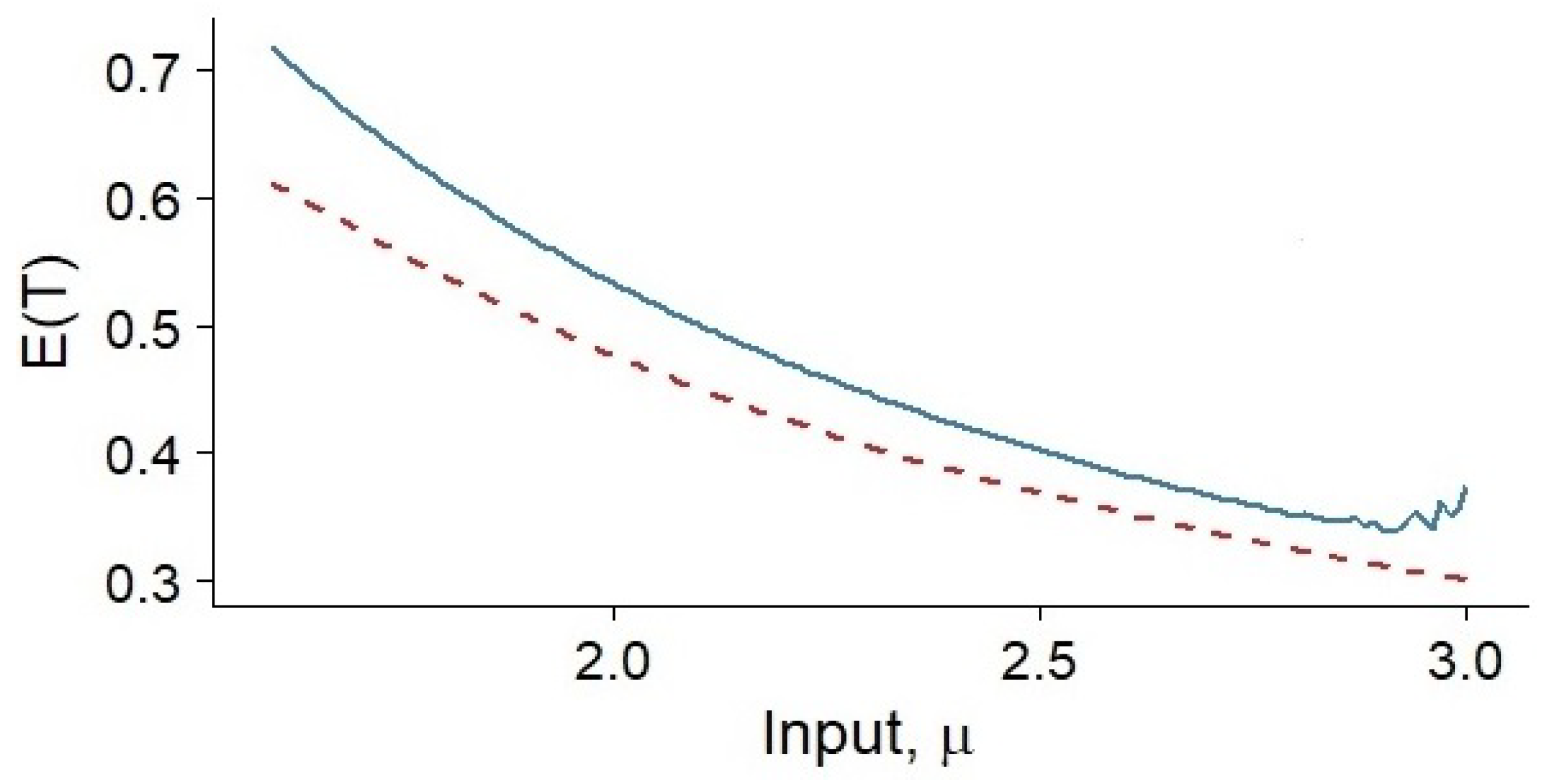
In Figure 1 we compare the mean FPT of the IGBM process obtained with the asymptotic expression (43) (red dashed line) and that given by the exact expression (6) (blue solid line) for $S=1$, $\sigma =0.8$, $\theta =1.1$, $x_0=0.2$, $V_I=0$.

We note that the proposed approximation slightly underestimates the value of $E\left(T\right)$, but the agreement of the two curves improves for larger $\mu$. Moreover for values of $\mu$ corresponding to strong external inputs the exact expression (6) is unstable, while the approximation is not.

In the following, we consider physiologically realistic parameter values as suggested in [19] and [46], with their unit measures. The resetting potential is chosen equal to zero, i.e., $x_0=0$ mV, the inhibitory reversal potential is $V_I=-10$ mV, and the firing threshold $S=10$ mV. The parameter of spontaneous decay towards the resting potential is chosen $\theta =5$ ms.

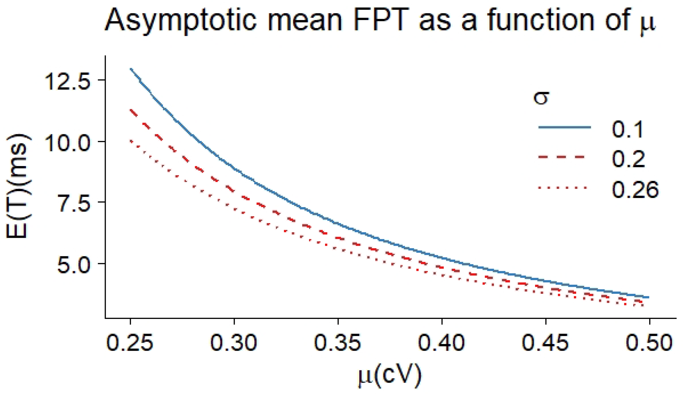
To check how sensitive is the asymptotic expression (43) to a change in $\mu$ or $\sigma$, we show the mean FPT as functions of the input for three different values of the noise amplitude in Figure 2.

As expected the mean waiting time before the first spike decreases as $\mu$ increases. Moreover, for fixed $\mu$, the mean FPT decreases for increasing $\sigma$ (see the plot from the top downwards).

The measure units of the neuronal membrane potential are usually expressed in millivolt, while here we use centivolt. It is just a simple rescale of the SDE (60) and does not affect the dynamics. The change of variable is used here as a numerical trick. In fact the series (43) is more computationally stable for small parameter $A_i$.

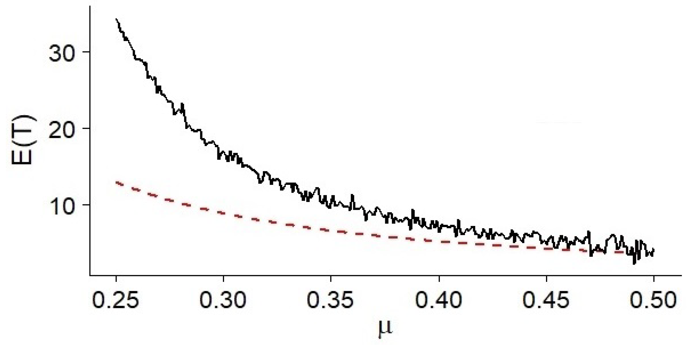
Finally, we observe that for the same computational accuracy, although non-optimal for small values of $\mu$, the approximated expression (43) is way more stable than the exact expression (6). For instance, in Figure 3 we compare the mean FPT obtained via the two formulas for $\sigma =0.2$ ms${}^{-1/2}$ and other parameters as in Figure 2.

Using the software environment R, for equal time and accuracy of the computation we observe that the asymptotic expression (43), for $\mu$ sufficiently large, is a more reliable tool for a numerical study of the firing rate.

4.2. Mean Reversion Models of Financial Markets

Mean reverting stochastic processes are often used in models of financial markets (see for instance [3,4,5,8,10,11,15,28]). The mean reversion property implies that the process tends to drive the short rate value towards the long term average level favoring upward (downward) movements if the short rate is too low (high). Among these processes the IGBM plays a relevant role: as GARCH diffusion process or Brennan and Schwartz model it is adopted to describe the value of real options, to study interest rates and to describe the underlying asset in the study of option prices in stochastic volatility models.

Here we want to investigate the sensitivity of the approximated mean FPT to a change in the threshold value S and in the instantaneous volatility $\sigma$. To avoid cumbersome calculations involving derivatives of hypergeometric functions with respect to the parameters, we display the main features of the approximated FPT through figures, using realistic parameters coming from the option-pricing literature.

We consider the model described by the following stochastic differential equation

$$d{X}_t=\lambda \left(\mu -X_t\right)dt+\sigma X_{t}d{W}_t,t>0X_0=x_0,$$

(61)

where $\mu >0$ represents the long-run mean, $\sigma$ is the instantaneous volatility, $W_t$ is a standard Wiener process and $\lambda$ is related to the speed of reversion towards the mean level. If $\lambda$ is large, on average it takes less time for the process to move around the long-run mean and more time to move towards points far from it, i.e., more likely the process will not move far away from the long-run mean level.

In the following, we consider realistic parameters values as suggested in [15] for Perpetual American Put Options: $\mu =3.25$, $\lambda =0.25$, $x_0=3$, ${\sigma }^2\in [0.08,0.2]$.

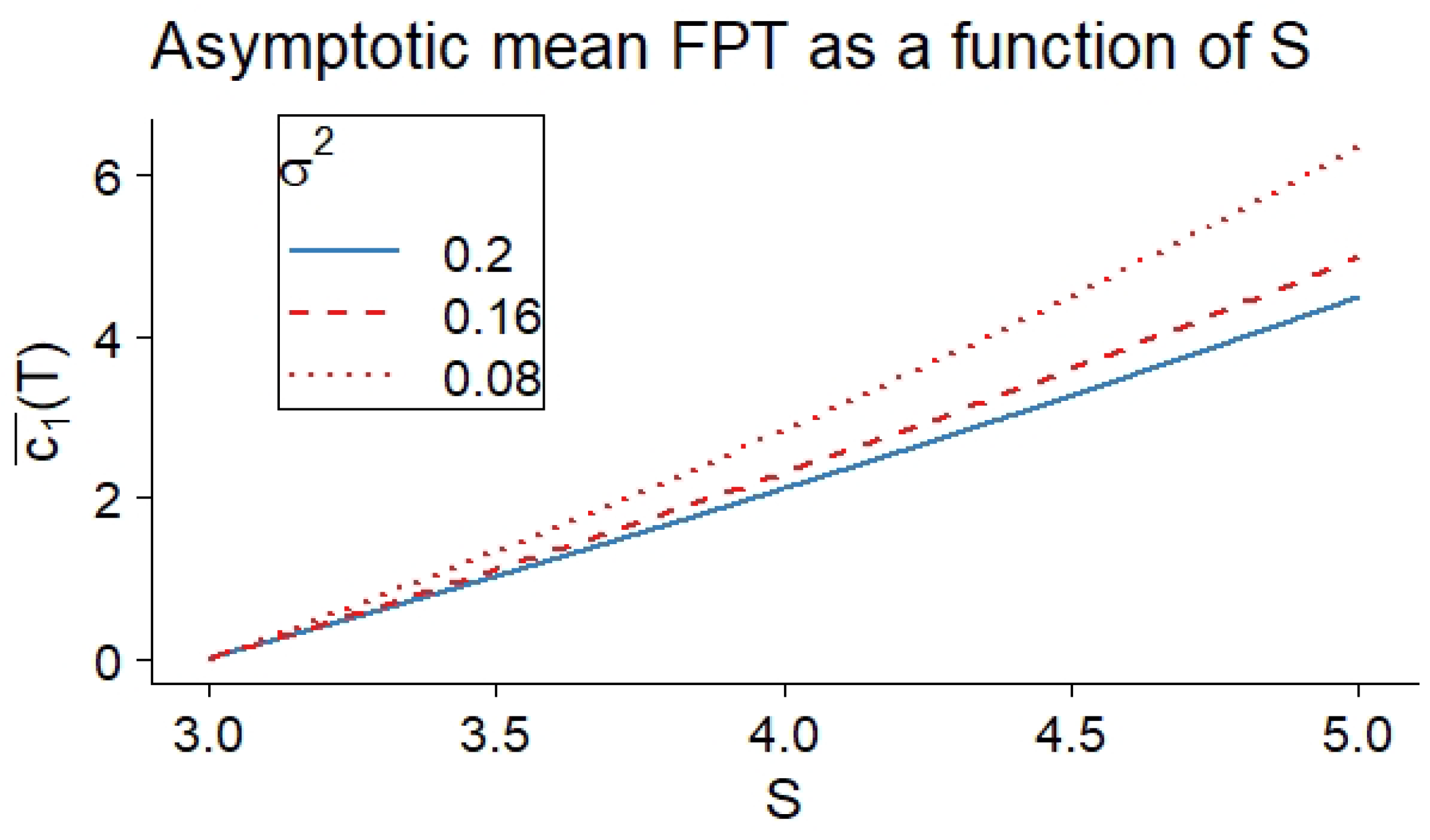
In Figure 4 we show for $X_t$ in Equation (61) the asymptotic first FPT cumulant given by Equation (43) as a function of S. The mean FPT for $S=3$ is equal to zero being, in this case, $S=x_0$, whereas, as expected, the mean time before the first crossing of S increases if the threshold moves away from $x_0$. Moreover, we observe that the mean FPT decreases for increasing values of the instantaneous volatility $\sigma$. In particular, if the long-run mean level is below S and $\lambda$ is large, $\sigma$ is the main factor that can favor the threshold crossing.

In

Table 1. Relative error between the asymptotic expression (43) and the mean FPT given by (6) for the same choices of parameters of Figure 4 and ${\sigma }^2=0.2$.

S	$\mathbb{E}\left(\mathit{T}\right)$	${\overline{\mathit{c}}}_1\left(\mathit{T}\right)$	$RelativeError$
$3.1$	$0.314$	$0.198$	$0.368$
$3.5$	$1.664$	$1.019$	$0.387$
$4.0$	$3.579$	$2.107$	$0.411$
$4.5$	$5.770$	$3.264$	$0.434$
$5.0$	$8.265$	$4.491$	$0.456$

we show the relative error

$$\frac{|\mathbb{E}\left(T\right)-{\overline{c}}_1\left(T\right)|}{\mathbb{E}\left(T\right)}$$

between the asymptotic expression (43) and the mean FPT given by (6) in the case ${\sigma }^2=0.2$ for five different choices of S. We observe that the asymptotic approximation underestimates slightly the waiting time before the first crossing. The error increases with S, although the relative error grows slowly. We note that the error is smaller for S close to $x_0$. The reason is that our approximation performs better for $A_1$, $A_2\to 0$ condition that, for fixed $\mu$, is better fulfilled if $x_0\simeq S$.

4.3. Conclusions and Open Problems

We addressed the problem of the first passage time T of the IGBM through a constant threshold, giving approximations of the cumulants of T of any order obtained from an asymptotic expansion of the Laplace transform of T using the algebra of formal power series. Moreover from the expression of the cumulants, $\left\{c_k\left(T\right)\right\}$, moments of T might be computed by using the recursion formula

$$\mathbb{E}\left[T^k\right]=c_k\left(T\right)+\sum _{i=1}^{k-1}\left(\genfrac{}{}{0pt}{}{k-1}{i-1}\right)c_i\left(T\right)\mathbb{E}\left[T^{k-i}\right].$$

(62)

We have shown that the approximations work better if the IGBM has a large positive drift or if the starting position of the dynamics is close to the threshold. Due to the lack of results in the literature about moments of T of order higher than 1, even though they hold only in a certain parameters range the cumulants approximations constitute a novel result and a step forward in the comprehension of the FPT problem for this diffusion process. The first two approximated cumulants are given explicitly in Corollaries 1 and 2. The higher-order cumulants can be obtained from Theorem 1 analytically or by means of the $\mathtt{R}$ symbolic-numeric procedure sketched at the beginning of Section 4 and based on the package $\mathtt{kStatistics}.$ We stress that the computational cost of this procedure is lighter than the one for the classical approach with the integro-differential equations, although a more in-depth numerical analysis should be carried out.

These results can be used in many applications ranging from neuronal modeling with reversal potential to mean reversion models of financial markets both for understanding the underlying dynamics of extreme events and possibly for the simultaneous estimation of parameters involved in the model. The examples we have given show that this approximation works better when $\mu$ is large or $x_0$ is close to $S.$

These last observations suggest using the cumulants (29) and the Laguerre-Gamma polynomial approximation proposed in [18] to get an estimation of the FPT pdf $g\left(t\right)$ for the range of parameters for which expression (9) holds. For large $t,$ the asymptotic results from [47] can be applied to obtain information on $g\left(t\right)$. Instead, for small-time $t,$ the approximation obtained through the expansion with Laguerre–Gamma polynomials and the cumulants (29) should result to be competitive when compared with the Monte Carlo methods and when traced back to $\mu$ large or $x_0$ close to $S.$ Indeed, the classical simulation schemes like Euler–Maruyama or Milstein method often provide uncorrected values of $g\left(t\right)$ around zero and so the approximation of $g\left(t\right)$ for small t turns out to be particularly relevant. This is on the agenda of our future research.

As the last remark, we stress that the methodology itself is not limited to the IGBM. As future work, we plan to extend this approach to other processes belonging to the class of Pearson’s diffusions, since the expression of the Laplace transform of the FPT pdf for these processes is often written as a ratio of two hypergeometric functions.