A Reliability Growth Process Model with Time-Varying Covariates and Its Application

Abstract

The nonhomogeneous Poisson process model with power law intensity, also known as the Army Materiel Systems Analysis Activity (AMSAA) model, is commonly used to model the reliability growth process of many repairable systems. In practice, it is necessary to test the reliability of the product under different operational environments. In this paper we introduce an AMSAA-based model considering the covariate effects to measure the influence of the time-varying environmental condition. The parameter estimation of the model is typically performed using maximum likelihood on the failure data. The statistical properties of the estimation in the model are comprehensively derived by the martingale theory. Further inferences including confidence interval estimation and hypothesis tests are designed for the model. The performance and properties of the method are verified in a simulation study, compared with the classical AMSAA model. A case study is used to illustrate the practical use of the model. The proposed approach can be adapted for a wide class of nonhomogeneous Poisson process based models.

1. Introduction

A repairable system is a system that can undergo reparation by mending or replacing some system components rather than re-establishing the entire system after failing. Most of the contemporary complex systems are repairable—for instance, communication systems, software systems, automobile engines, helicopters, and aircraft generators all belong to the repairable category. The reliability of some repairable systems can be improved by a test, analyze, and fix process, where system failures are identified and corrective actions are implemented until the reliability reaches a prespecified level. This procedure of improvement is called the reliability growth process, or the reliability growth test.

The reliability growth test is a powerful tool to improve repairable system’s reliability by identifying and repairing failure units, which has been widely used in many industries [1]. In the testing, data of failure times are collected to assess the changing trend of the product’s reliability growth. A variety of reliability models have been developed to study these testing data. Duane [2] first introduced the reliability growth model for aircraft engines by using the learning curve to describe the relationship between the cumulative failure rate and the cumulative testing time. Crow [3] further delved into the stochastic extension of Duane’s model, where failures can be represented as a nonhomogeneous Poisson process (NHPP) with Weibull intensity, which is also called a power law process [4]. The developed model is now known as the Army Materiel Systems Analysis Activity (AMSAA) model and has been popular, with multiple applications in industrial areas including automobiles [5], health care [6], power systems [7], and coal mining [8]. Subsequently, more forms of the NHPP model have been introduced to characterize the time-varying rates, such as the log-linear intensity model [9] and the exponential-trigonometric intensity model [10]. The statistical theory of the classical AMSAA model has been intensively studied as well. Some of these efforts focused on confidence interval estimation [11,12], future reliability estimation [13], first passage time problem [14], model selection [15] and goodness-of-fit test [16].

More recently, an increasing number of extensions of the AMSAA model have been proposed to foster product development. For instance, Somboonsavatdee et al. [17] investigated the statistical inference of the AMSAA model under competing risks; Peng et al. [18] proposed a novel method to evaluate and predict the dynamic reliability of a repairable system subjected to the interval-censoring problem based on the AMSAA model; Hu et al. [19] designed a robust decision method for the planning of reliability growth testing by integrating information gap decision theory and the AMSAA model. A compelling improvement to the AMSAA model is the incorporation of heterogeneity—an inclusion of individual-specific factors or covariates that may affect the reliability growth process. To measure the impact of operational and environmental factors, it is essential to take covariate effects into consideration, and several studies have already displayed this awareness. Van Dyck and Verdonck [20] extended the AMSAA model by introducing a multiplicative covariate factor with the interpretation of a known scaling of the system’s failure character. Similarly, Slimacek and Lindqvist [21] introduced a novel approach for the statistical modeling of failures where nonparametric frailty and covariates were considered in the NHPP model. In addition to the NHPP-based models, proportional hazard models are also able to delineate the covariate effects; however, they make no distributional assumptions about the failure process [22].

Among all the contemporary analyses of repairable systems with covariates or environmental effects, the majority are conducted over reliability growth tests for multiple experimental individuals, machines, or systems. However, with the present rising reliability requirements and the increasing product useful life, the cost of conducting reliability growth tests often becomes exorbitant. Because test costs and the availability of test subjects can sometimes be a barrier to the progression of reliability growth tests, it is more practical and economical to conduct tests with a single test subject under different experimental conditions; in other words, it would be more desirable if the covariates were time-dependent and the data were collected from one sample path. These time-varying covariates can include local climatic conditions like temperature and humidity or operational factors like current intensity and rotating speed, which can all be dynamically monitored during the test. To our best knowledge, there have been few comprehensive investigations on the AMSAA model with such test settings. In this paper, we model the data of a reliability growth test in a time-varying environment through an extended AMSAA model.

In a classical AMSAA model, the parameters can be estimated by using maximum likelihood estimation (MLE) with analytic forms, whose exact distributions can be derived as chi-square distributions [3]. However, since there is no analytic form for MLE in the extension, it is challenging to discuss the properties of MLE. Moreover, most NHPP-based works on repairable systems develop estimations and inferences from the classical MLE theory, which is not readily applicable to small sample data with dependence. With these previous limitations in mind, the statistical properties of MLE and further inferences of the model are derived comprehensively from the martingale theory in the present study. The rest of this paper is organized as follows. In Section 2, we establish the AMSAA model with time-varying covariates of environmental effects. The method and property of the parameter estimation are discussed in Section 3. More statistical inference paradigms are developed in Section 4. A comprehensive simulation study and a case study are described in Section 5 and Section 6. A final discussion and an overview of the study are presented in Section 7.

2. AMSAA Model with Time-Varying Covariates

When evaluating the reliability of complex repairable systems with counting process models, each event in the process represents one instance of a failure of the system. The counting process $\{N(t),t\ge 0\}$ is said to be a nonhomogeneous Poisson process with intensity function $\lambda (t)$, $t\ge 0$ if it satisfies:

• $N(0)=0$;
• $N(t)$ has independent increments;
• $P(N(t+h)-N(t)\ge 2)=o(h)$;
• $P(N(t+h)-N(t)=1)=\lambda (t)h+o(h)$.

Under the conditions in the definition of NHPP, the distribution of the number of events that occurred in $(s,t]$, $N(t)-N(s)$, can be obtained from:

$$P(N(t)-N(s)=k)=\frac{1}{k!}{[\mathsf{\Lambda }(t)-\mathsf{\Lambda }(s)]}^k{e}^{-[\mathsf{\Lambda }(t)-\mathsf{\Lambda }(s)]},$$

(1)

where $\mathsf{\Lambda }(t)=E[N(t)]={\int }_0^t\lambda (u)\mathrm{d}u$. Let $N(t^{-})$ denote the number of events that occurred before time t. If we observe n events in the interval $[0,T]$ and the events occurred at times $t_1,t_2,\cdots ,t_n$, the desired joint probability density function with $t_0=0$ takes the form,

$$\begin{array}{cc}\hfill f(t_1,t_2,\cdots ,t_n)& =\prod _{i=1}^{n}P\left(N(t_i^{-})-N(t_{i-1})=0,N(t_i)-N(t_i^{-})=1\right)P(N(T)-N(t_n)=0)\hfill \\ \hfill & =\prod _{i=1}^n{e}^{-\mathsf{\Lambda }(t_i)+\mathsf{\Lambda }(t_{i-1})}\lambda (t_i)e^{-\mathsf{\Lambda }(T)+\mathsf{\Lambda }(t_n)}\hfill \\ \hfill & =\prod _{i=1}^n\lambda (t_i)e^{-\mathsf{\Lambda }(T)}.\hfill \end{array}$$

(2)

Several forms of the intensity function have been used in modeling the process of reliability growth. In the present study, we considered the celebrated power law intensity adopted in AMSAA model, that is, $\lambda (t)=\gamma \alpha t^{\alpha -1}$. The expected event number up to time t is $\gamma t^{\alpha }$.

When operating the testing machine in environmental or operational conditions that are dynamic, external factors (e.g., temperature and stress) and internal factors (e.g., speed) will influence the reliability growth process of the machine. Now suppose that for the system there is a d-dimensional time-dependent covariate vector $\mathit{X}(t)$ that affects the intensity of events’ occurrence. Note that $\mathit{X}(t)$ may be deterministic or random, continuous or discrete about testing time. A deterministic and discrete situation is the most common due to the multi-stage experiment design, where the experimental conditions are changed in each stage. To quantify the reliability growth process with time-dependent covariate effects, some assumptions are made for the model.

Assumption 1.

$\mathit{X}(t)$ is right-continuous with limits from the left and bounded almost surely.

Assumption 2.

The base reliability growth process under a standard condition evolves as a power law process.

Assumption 3.

$\mathit{X}(t)$ impacts the failure intensity by a multiplicative factor $e^{{\mathit{\beta }}^T\mathit{X}(t)}$, where $\mathit{\beta }$ is a d-dimensional constant vector.

Assumption 1 is satisfied in most cases in reality. Usually, $\mathit{X}(t)$ is the monitoring data, which can be observed up to time t. The bounding condition restricts the covariate effect within a reasonable range so that the expected failure will tend to infinity as the operational time tends to infinity. Assumption 2 is also a common assumption that characterizes evolving pattern of a product’s reliability with normal use. In Assumption 3, the model we consider for the inclusion of $\mathit{X}(t)$ is of the Cox type. This gives us the intensity and the expectation function with covariate effects respectively:

$$\begin{array}{c}\lambda (t)=\gamma \alpha t^{\alpha -1}{e}^{{\mathit{\beta }}^T\mathit{X}(t)},\\ \mathsf{\Lambda }(t)={\int }_0^t\gamma \alpha u^{\alpha -1}{e}^{{\mathit{\beta }}^T\mathit{X}(u)}\mathrm{d}u.\end{array}$$

(3)

In the model, $\alpha$, $\gamma$, and $\beta$ are unknown parameters, with $\alpha$ and $\gamma$ being positive. As a well-known property of the counting process, we have the following martingale property for the model.

Property 1.

$N(t)-\mathsf{\Lambda }(t)$ is a square integrable martingale with respect to the filtration ${\mathcal{F}}_t=\sigma \{N(s),s\le t\}$, and its predictable variation process is $\mathsf{\Lambda }(t)$.

Further properties and theories of the counting process and martingale can be found in [23].

3. Maximum Likelihood Estimation

The maximum likelihood method is considered for estimating the unknown parameters $\gamma ,\alpha$, and $\mathit{\beta }$. The log-likelihood of (2) is given by

$$l_T(t_1,t_2,\cdots ,t_n;\gamma ,\alpha ,\mathit{\beta })=nlog\gamma +nlog\alpha +{\mathit{\beta }}^T\sum _{i=1}^n\mathit{X}(t_i)+(\alpha -1)\sum _{i=1}^{n}log(t_i)-{\int }_0^T\gamma \alpha t^{\alpha -1}{e}^{{\mathit{\beta }}^T\mathit{X}(t)}\mathrm{d}t.$$

(4)

Then, the estimation values can be obtained by the optimization problem,

$$(\widehat{\gamma },\widehat{\alpha },\widehat{\mathit{\beta }})=arg\underset{(\gamma ,\alpha ,\mathit{\beta })}{max}{l}_T(t_1,t_2,\cdots ,t_n;\gamma ,\alpha ,\mathit{\beta }).$$

(5)

The first-order partial derivatives of the log-likelihood are

$$\begin{array}{cc}\frac{\partial l_T}{\partial \gamma }\hfill & =\frac{n}{\gamma }-{\int }_0^T\alpha t^{\alpha -1}{e}^{{\mathit{\beta }}^T\mathit{X}(t)}\mathrm{d}t,\hfill \end{array}$$

(6)

$$\begin{array}{cc}\frac{\partial l_T}{\partial \mathit{\beta }}\hfill & =\sum _{i=1}^n\mathit{X}(t_i)-{\int }_0^T\mathit{X}(t)\gamma \alpha t^{\alpha -1}{e}^{{\mathit{\beta }}^T\mathit{X}(t)}\mathrm{d}t,\hfill \end{array}$$

(7)

$$\begin{array}{cc}\frac{\partial l_T}{\partial \alpha }\hfill & =\frac{n}{\alpha }+\sum _{i=1}^{n}log(t_i)-{\int }_0^T\gamma t^{\alpha -1}{e}^{{\mathit{\beta }}^T\mathit{X}(t)}\mathrm{d}t-{\int }_0^{T}log(t)\gamma \alpha t^{\alpha -1}{e}^{{\mathit{\beta }}^T\mathit{X}(t)}\mathrm{d}t.\hfill \end{array}$$

(8)

The parameter estimation can be computed by setting the partial derivatives equal to zero and solving the equations. However, there is one key problem that requires discussion before the computation—the existence and uniqueness of the solution. We will prove the property by constructing conditional likelihood.

Consider the conditional distribution of $t_1,t_2,\cdots ,t_n$ given $N(T)=n$. The conditional distribution is given by the distribution of the order statistics of the random variable t whose density function is $\frac{\lambda (t)}{\mathsf{\Lambda }(T)}$. Note that the distribution function does not contain the parameter $\gamma$. As a result, the conditional log-likelihood function is given by

$$l(t_1,t_2,\cdots ,t_n|N(T)=n;\alpha ,\mathit{\beta })=\alpha \sum _{i=1}^{n}log(t_i)+{\mathit{\beta }}^T\sum _{i=1}^n\mathit{X}(t)-nlog{\int }_0^T{t}^{\alpha -1}{e}^{{\mathit{\beta }}^T\mathit{X}(t)}\mathrm{d}t.$$

(9)

We have the following lemma for the conditional log-likelihood.

Lemma 1.

The maximum likelihood estimator for the log-likelihood (9) exists and is unique with probability 1 as the time tends to infinity. Moreover, the estimator is strongly consistent.

Proof. 

The problem is equal to discussing the existence and uniqueness of the maximum likelihood estimation of the parameters for n independent and identically distributed random variables with density function $\frac{\lambda (t)}{\mathsf{\Lambda }(T)}$. Furthermore, $\frac{\lambda (t)}{\mathsf{\Lambda }(T)}$ is an exponential distribution family with natural parameter α and $\mathit{\beta }$. Note that $N(T)\to \infty$ with probability 1 as $T\to \infty$. Then, the property in the lemma is derived by the theory of classical repeated sampling from an exponential family [24]. □

The estimator in the lemma gives the same solution with that of (5) for $\alpha$ and $\mathit{\beta }$. We will prove the existence, uniqueness and consistency for the estimator of full log-likelihood in the following theorem.

Theorem 1.

The maximum likelihood estimator from (5) exists and is unique with probability 1 as the time tends to infinity. Moreover, the estimator is strongly consistent.

Proof. 

The estimation for $\widehat{\alpha }$ and $\widehat{\mathit{\beta }}$ in optimization (5) is equal to maximizing the conditional likelihood (9), which derives from the direct calculations shown in Appendix A. Due to the analytic form of $\widehat{\gamma }$ with $\alpha$ and $\mathit{\beta }$ given by (10), the existence and uniqueness are held for (5). The strong consistency of $\widehat{\alpha }$ and $\widehat{\mathit{\beta }}$ is given by Lemma 1.

$$\widehat{\gamma }=\frac{n}{{\int }_0^T\widehat{\alpha }{t}^{\widehat{\alpha }-1}{e}^{{\widehat{\mathit{\beta }}}^T\mathit{X}(t)}\mathrm{d}t}.$$

(10)

As shown in Property 1, $N(T)-\mathsf{\Lambda }(T)$ is a square integrable martingale, whose predictable variation process is $\mathsf{\Lambda }(T)$. By Liptser’s law of large numbers for martingales [25], we have

$$\frac{N(T)-\mathsf{\Lambda }(T)}{\mathsf{\Lambda }(T)}\to 0,T\to \infty$$

(11)

almost surely on $\left\{\mathsf{\Lambda }(\infty )=\infty \right\}$. With the discussion on Assumption 1, we know that $\mathsf{\Lambda }(\infty )=\infty$ holds almost surely. Then, with the consistency of $\widehat{\alpha }$ and $\widehat{\mathit{\beta }}$,

$$\widehat{\gamma }=\gamma \frac{N(T)}{\mathsf{\Lambda }(T;\widehat{\alpha },\widehat{\mathit{\beta }})}\to \gamma ,T\to \infty$$

(12)

almost surely, where $\mathsf{\Lambda }(T;\widehat{\alpha },\widehat{\mathit{\beta }})$ denotes the expectation function with parameters $\gamma ,\widehat{\alpha }$, and $\widehat{\mathit{\beta }}$. Hence, $\widehat{\gamma }$ is strongly consistent. □

With all the proofs above, the full log-likelihood function of the observations can be factorized as follows:

$$l_T(t_1,t_2,\cdots ,t_n;\gamma ,\alpha ,\mathit{\beta })=l(t_1,t_2,\cdots ,t_n;|N(T)=n;\alpha ,\mathit{\beta })+l(n;\gamma ,\alpha ,\mathit{\beta }),$$

(13)

where, $l(t_1,t_2,\cdots ,t_n;|N(T)=n;\alpha ,\mathit{\beta })$ is given by (9) and

$$\begin{array}{c}\hfill l(n;\gamma ,\alpha ,\mathit{\beta })=-{\int }_0^T\gamma t^{\alpha -1}{e}^{{\mathit{\beta }}^T\mathit{X}(t)}\mathrm{d}t+nlog{\int }_0^T\gamma t^{\alpha -1}{e}^{{\mathit{\beta }}^T\mathit{X}(t)}\mathrm{d}t.\end{array}$$

(14)

Then, the optimization (5) can be factorized as follows, which may help to simplify the numerical calculation in practice.

$$\begin{array}{cc}\hfill & \widehat{\alpha },\widehat{\mathit{\beta }}=arg\underset{\alpha ,\mathit{\beta }}{max}l(t_1,t_2,\cdots ,t_n|N(T)=n;\alpha ,\mathit{\beta }),\hfill \end{array}$$

(15)

$$\begin{array}{cc}\hfill & \widehat{\gamma }=arg\underset{\gamma }{max}l(n;\gamma ,\widehat{\alpha },\widehat{\mathit{\beta }}).\hfill \end{array}$$

(16)

4. Statistical Inference

In this section, we will discuss the distribution of the maximum likelihood estimation, which is expected to be asymptotically normal in most cases, as well as some inferences for the proposed model.

4.1. Asymptotic Normality of the Parameter Estimation

Before discussing normality, we present the martingale property of the score function.

Property 2.

Denote ${(\gamma ,\alpha ,\mathit{\beta })}^T$ by θ. The score function $\frac{\partial l_T}{\partial \theta }$ denoted by ${\dot{l}}_T(\theta )$ is a square integrable martingale with mean zero with respect to the filtration ${\mathcal{F}}_T=\sigma \{N(s),s\le T\}$.

The property follows from the fact that ${\dot{l}}_T(\theta )$ can be formulated as ${\int }_0^{T}H(t)(\mathrm{d}N(t)-\mathrm{d}\mathsf{\Lambda }(t))$. The specific form of $H(t)$ can be extracted from (6), (7), and (8). With this property, the asymptotic normality of the maximum likelihood estimator can now be deduced by standard arguments.

Theorem 2.

Suppose $\widehat{\theta }$ is the maximum likelihood estimator given by (5). Then,

$$I_T{(\theta )}^{\frac{1}{2}}(\widehat{\theta }-\theta )\stackrel{d}{⟶}N(0,\mathrm{I})$$

(17)

as $T\to \infty$, where $I_T(\theta )=-E_{\theta }\left[\frac{{\partial }^2{l}_T}{\partial \theta \partial {\theta }^T}\right]$ and $\mathrm{I}$ is the identity matrix.

Proof. 

On series expansion, we see that

$${\dot{l}}_T(\theta )=J_T(\tilde{\theta })(\theta -\widehat{\theta }),$$

(18)

where $J(\tilde{\theta })=-\frac{{\partial }^2{l}_T}{\partial \theta \partial {\theta }^T}{|}_{\theta =\tilde{\theta }}$ and $\tilde{\theta }$ is a convex combination of ${(\gamma ,\alpha ,\mathit{\beta })}^T$ and ${(\widehat{\gamma },\widehat{\alpha },\widehat{\mathit{\beta }})}^T$. Therefore,

$$\begin{array}{cc}\hfill I_T{(\theta )}^{-\frac{1}{2}}{\dot{l}}_T(\theta )& =I_T{(\theta )}^{-\frac{1}{2}}{J}_T(\tilde{\theta })(\theta -\widehat{\theta })\hfill \end{array}$$

(19)

$$\begin{array}{cc}\hfill & =I_T{(\theta )}^{-\frac{1}{2}}(J_T(\tilde{\theta })-I_T(\theta )+I_T(\theta ))(\theta -\widehat{\theta })\hfill \end{array}$$

(20)

$$\begin{array}{cc}\hfill & =(A+\mathrm{I})I_T{(\theta )}^{\frac{1}{2}}(\widehat{\theta }-\theta ),\hfill \end{array}$$

(21)

where

$$A=I_T{(\theta )}^{-\frac{1}{2}}(J_T(\tilde{\theta })-I_T(\theta ))I_T{(\theta )}^{-\frac{1}{2}}.$$

(22)

It follows from the central limit theorem for martingales [26] that

$$I_T{(\theta )}^{-\frac{1}{2}}{\dot{l}}_T(\theta )\stackrel{d}{⟶}N(0,\mathrm{I}),T\to \infty .$$

(23)

Because $I_T(\theta )$ and $J_T(\theta )$ are asymptotically equivalent and the consistency of $\widehat{\theta }$, A tends to zero in probability as $T\to \infty$. Therefore, we get the asymptotic normality of $I_T{(\theta )}^{\frac{1}{2}}(\widehat{\theta }-\theta )$. □

Remark 1.

$I_T(\theta )$ and $J_T(\theta )$ are well known as the expected information matrix and observed information matrix, respectively. The concrete forms are displayed in Appendix B. Due to the asymptotic equivalence of these two information matrices, $I_T(\theta )$ in the theorem can be replaced by $J_T(\theta )$.

4.2. Inference of MTBF

The mean time between failures (MTBF) describes the expected time between two failures for a repairable system, and is a very important indicator in the process of reliability growth. Under the setting of NHPP, the mean time between failures at time t, $MTB{F}_t$, is $\frac{1}{\lambda (t)}$. With the parameters estimated, the estimation of $MTB{F}_t$ can be given by

$$\widehat{MTB{F}_t}=\frac{1}{\widehat{\lambda }(t)}=\frac{1}{\widehat{\gamma }\widehat{\alpha }{t}^{\widehat{\alpha }-1}{e}^{{\widehat{\mathit{\beta }}}^T\mathit{X}(t)}}.$$

(24)

$\widehat{MTB{F}_t}$ is a continuous and differentiable function of $\widehat{\theta }$. The distribution of $\widehat{MTB{F}_t}$ can be given by the delta method as:

$$\widehat{MTB{F}_t}\sim N\left(\frac{1}{\lambda (t)},g^T(\theta )I_T^{-1}(\theta )g(\theta )\right),$$

(25)

where

$$\begin{array}{cc}\hfill g^T(\theta )& =\frac{\partial MTB{F}_t}{\partial {\theta }^T}\hfill \\ \hfill & =\left(-\frac{1}{{\gamma }^2\alpha t^{\alpha -1}{e}^{{\mathit{\beta }}^T\mathit{X}(t)}},-\frac{t^{\alpha -1}+\alpha t^{\alpha -1}logt}{\gamma {(\alpha t^{\alpha -1})}^2{e}^{{\mathit{\beta }}^T\mathit{X}(t)}},-\frac{\mathit{X}(t)e^{{\mathit{\beta }}^T\mathit{X}(t)}}{\gamma \alpha t^{\alpha -1}{(e^{{\mathit{\beta }}^T\mathit{X}(t)})}^2}\right).\hfill \end{array}$$

(26)

Then, the $95\%$ confidence interval estimation of $MTB{F}_t$ can be computed in the form by plugging in $\widehat{\theta }$,

$$\left[\frac{1}{\widehat{\lambda }(t)}-q_{97.5\%}\sqrt{g^T(\widehat{\theta })I_T^{-1}(\widehat{\theta })g(\widehat{\theta })},\frac{1}{\widehat{\lambda }(t)}+q_{97.5\%}\sqrt{g^T(\widehat{\theta })I_T^{-1}(\widehat{\theta })g(\widehat{\theta })}\right],$$

(27)

where $q_{97.5\%}$ is the $97.5$th percentile of the standard normal distribution.

Note that the $MTB{F}_t$ is a transient index computed under the time dimension of the accelerated reliability growth test, where the accelerated factor is decided by the covariate effects. In practice, we also want to know what the reliability of the machine would be like if there have been $\mathsf{\Lambda }(t)$ faults fixed in normal use; such a reliability can be inferred from the MTBF at $t^{(0)}$ in a standard condition test, where the expected cumulative number of failures at t under covariate effects is equal to the expected cumulative number of failures at $t^{(0)}$ under the standard conditions.

To distinguish between the two MTBF types, we will use $MTB{F}^{(0)}$ to denote the latter. There exists a measurable map $\psi$ from the test time t with covariate effects to the equivalent time $t^{(0)}$ in the standard condition so that the transformed process denoted by $\{N(t^{(0)}),t\ge 0\}$ is an NHPP with intensity function ${\lambda }^{(0)}(t^{(0)})=\gamma \alpha {(t^{(0)})}^{\alpha -1}$ and expectation function ${\mathsf{\Lambda }}^{(0)}(t^0)=\gamma {(t^{(0)})}^{\alpha }$. The aforementioned setup yields:

$$\psi (t)=\{t^{(0)}|{\mathsf{\Lambda }}^{(0)}(t^{(0)})=\mathsf{\Lambda }(t)\}={\gamma }^{-\frac{1}{\alpha }}\mathsf{\Lambda }{(t)}^{\frac{1}{\alpha }}.$$

(28)

Subsequently, the estimated $MTB{F}^{(0)}$ for the testing time t in the test with covariate effects is

$${\widehat{MTBF}}_{\psi (t)}^{(0)}=\frac{1}{\widehat{\gamma }\widehat{\alpha }{(\psi (t;\widehat{\theta }))}^{\widehat{\alpha }-1}}={\gamma }^{-\frac{1}{\widehat{\alpha }}}{\widehat{\alpha }}^{-1}\mathsf{\Lambda }{(t;\widehat{\theta })}^{\frac{1}{\widehat{\alpha }}-1}.$$

(29)

The $95\%$ confidence interval is given by

$$\left[{\widehat{MTBF}}_{\psi (t)}^{(0)}-q_{97.5\%}\sqrt{g_{*}^T(\widehat{\theta })I_T^{-1}(\widehat{\theta })g_{*}(\widehat{\theta })},{\widehat{MTBF}}_{\psi (t)}^{(0)}+q_{97.5\%}\sqrt{g_{*}^T(\widehat{\theta })I_T^{-1}(\widehat{\theta })g_{*}(\widehat{\theta })}\right],$$

(30)

where $g_{*}(\widehat{\theta })=\frac{{\widehat{MTBF}}_{\psi (t)}^{(0)}}{\partial \widehat{\theta }}$.

Furthermore, we generalize the MTBF to the situation where $\mathsf{\Lambda }(t)$ faults have been fixed for the machine under the covariate effects of $e^{{\mathit{\beta }}_Y^T\mathit{Y}(t)}$, with parameter ${\mathit{\beta }}_Y$ being known. A new map ${\psi }_Y(t)$ for the testing time is constructed in a similar manner to that of (28),

$${\psi }_Y(t)=\{t^{(Y)}|{\mathsf{\Lambda }}^{(Y)}(t^{(Y)})=\mathsf{\Lambda }(t)\},$$

(31)

where ${\mathsf{\Lambda }}^{(Y)}(t^{(Y)})={\int }_0^{t^{(Y)}}\gamma \alpha u^{\alpha -1}{e}^{{\mathit{\beta }}_Y^T\mathit{Y}(u)}\mathrm{d}u$. Note that the map is one-to-one due to the monotonically increasing property of ${\mathsf{\Lambda }}^{(Y)}(·)$. Therefore, the estimation for $MTB{F}_{{\psi }_Y(t)}^{(Y)}$ is

$${\widehat{MTBF}}_{{\psi }_Y(t)}^{(Y)}=\frac{1}{\widehat{\gamma }\widehat{\alpha }{({\psi }_Y(t;\widehat{\theta }))}^{\widehat{\alpha }-1}{e}^{{\widehat{\mathit{\beta }}}_Y^T\mathit{Y}({\psi }_Y(t;\widehat{\theta }))}}.$$

(32)

In addition, the $95\%$ confidence interval can be given by the delta method, as shown in (27) and (30).

4.3. Hypothesis Test for Covariate Effects

The inference of the covariate effects can be accomplished by using likelihood ratio tests. Consider the hypothesis test problem,

$$H_0:{\mathit{\beta }}_S=0v.s.H_1:{\mathit{\beta }}_S\ne 0,$$

where $S\subseteq \{1,2,\cdots ,d\}$. The test aims to check whether the covariates in the subset S influence the reliability growth process significantly. The likelihood ratio test is designed to achieve this purpose. The likelihood ratio statistic can be given by

$$LR=\frac{{sup}_{{\mathit{\beta }}_{-S},\alpha }f(t_1,t_2,\cdots ,t_n|N(T)=n;\alpha ,{\mathit{\beta }}_{-S},{\mathit{\beta }}_S=\mathbf{0})}{{sup}_{\mathit{\beta },\alpha }f(t_1,t_2,\cdots ,t_n|N(T)=n;\alpha ,\mathit{\beta })}$$

(33)

where ${\mathit{\beta }}_{-S}$ represents the vector excluding ${\mathit{\beta }}_S$. By Wilks’ theorem, under $H_0$, $-2logLR$ has an asymptotic distribution of ${\chi }_{\left|S\right|}^2$, where $\left|S\right|$ is the cardinal number of the set S. Then, the null hypothesis will be rejected at a significance level of $0.05$ if $-2logLR$ is greater than the 95th percentile of ${\chi }_{\left|S\right|}^2$, indicating that the covariate effects of ${\mathit{X}}_S(t)$ are significant.

5. Simulation Study

The functionalities of the proposed model and estimation method are validated in the simulation study. Data of time points when failures happen are simulated by a non-homogeneous Poisson process whose intensity function is defined as (3). The time-dependent covariate effect is considered as a step function which occurs when the environmental factor (e.g., temperature) is changed as designed at some points during the test. The values of the step function are defined in Table 1.

Table 1. Step covariate function.

Time	[0, 10,000)	[10,000, 25,000)	[25,000, 50,000)	[50,000, 100,000]
$\mathit{X}(t)$	0	0.8	0.5	0.3

The parameters in the model are set as, $\gamma =1$, $\alpha =0.5$, and $\beta =1$. The failure points of the process are generated by the thinning approach [27], which applies thinning to the points generated from a homogeneous Poisson process with a rate parameter equal to the maximum of the intensity function. MLE is done for the simulated data and the procedure is repeated 1000 times. The estimation results are summarized in Table 2.

Table 2. Simulation results.

Parameter	Mean	Standard Deviation	Theoretical Standard Deviation	Mean Square Error
$\gamma$	0.9744	0.3168	0.3285	0.101
$\alpha$	0.5066	0.0295	0.0295	0.0009
$\beta$	0.9966	0.1741	0.1741	0.0303

From the results, we can conclude that the MLE results are close to the true values, with relatively small mean square errors (MSEs). The standard deviations of the estimates almost perfectly match the theoretical standard deviations computed from the square root of the inverse of the expected information matrix. As a means of comparison, the classical AMSAA model without considering the covariate effects is fitted as well. This model has a mean of 0.66 and a standard deviation of 0.1991 for $\widehat{\gamma }$; the mean of $\widehat{\alpha }$ is 0.5728 with a standard deviation of 0.0263. The deviation between the estimation of the classical AMSAA model and the true parameters $(\gamma ,\alpha )$ in the base intensity is perceptibly large. In order to further compare the performance in fitting the reliability growth trend, the fitted intensity functions are plotted with the means of MLEs in Figure 1. The curve of the intensity estimated by the AMSAA model with covariate effects is within the $95\%$ confidence band, while the curve of the classical AMSAA model deviates considerably large from the true curve. The comparison result again tellingly emphasizes the indispensability of considering covariate effects.

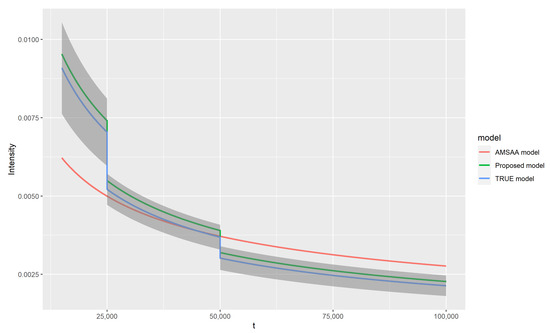
Figure 1. Intensity functions on $[15,000,100,000]$ in different models. The grey area is the $95\%$ confidence band constructed by the true parameters. For the sake of comparison and neatness, the confidence band is constructed around the true curve rather than the two estimated curves. The band width is the same as that of the proposed model, which is computed with the delta method by plugging in the true parameter values.

Another aspect in the simulation study that calls for verification is the normality of the estimators. The quantile-quantile (Q-Q) plot method is employed to show the distributions of $\widehat{\gamma }$, $\widehat{\alpha }$, and $\widehat{\beta }$, which are presented in Figure 2. As expected, the scattered points are distributed around the line $y=x$ except for the most extreme values, and this pattern indicates a good fit. Therefore, it is plausible to conclude that the estimator is approximately normally distributed in practice.

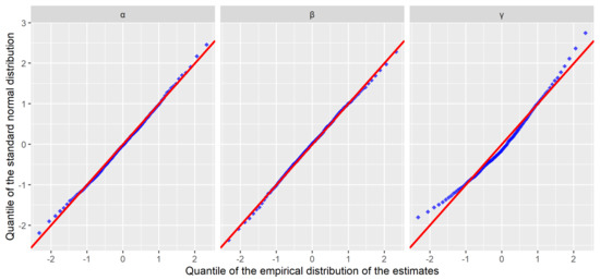
Figure 2. Quantile-quantile plot. The quantiles of the the empirical distributions are calculated with the normalized estimation results.

The relationship between MSE, which is computed by the mean square $l_2$ norm of $\widehat{\theta }-\theta$, and testing time is studied as well. The maximum testing time is increased from $\mathrm{100,000}$ to $\mathrm{600,000}$ with a step size of $\mathrm{50,000}$. The testing time of each phase is increased proportionally. For each testing time, the procedure of simulation and estimation is repeated 1000 times. As seen in Figure 3, MSE decreases with the increase of testing time, which illustrates the consistency of the estimates.

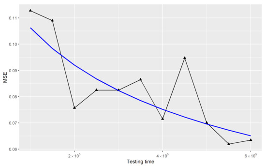
Figure 3. The relationship between mean square error (MSE) and testing time. The blue curve is the trend line fitted by the formula $y=\frac{1}{\sqrt{a+bx}}$.

6. Case Study

The data used in the case study is obtained from a real dataset collected in a reliability growth test during the development phase of an engine. In the test, the engine was tested in four phases with different operational conditions, and the failure times were recorded. Some summary statistics are provided in Table 3.

Table 3. Description of the dataset.

	Phase 1	Phase 2	Phase 3	Phase 4
Time (hour)	[0,230)	[230,1687)	[1687,3764)	[3764,5303]
Number of failures	17	36	58	16
Covariate	0	1	2	0

In this particular case, it is impossible to monitor all aspects of the environment. So, the covariate in table is generated from scoring by experts, and is the evaluation for the stress intensity of the environment. More specially, the testers rate the stress intensity of the experimental environment as $\{\mathrm{0,1,2}\}$ based on the sensitive parameters of the engine, such as gas pressure, temperature, and rotation speed.

We estimate the parameters by maximizing the log-likelihood. The estimation results are shown in Table 4. The value $\widehat{\alpha }$ is less than 1, which suggests that the reliability of the machine is improved in the testing procedure. The positive $\widehat{\beta }$ implies that the increase in the stress intensity of the environment accelerates the process of the fault exposure.

Table 4. Estimation results.

Parameter	Estimation	Standard Deviation
$\gamma$	0.3511	0.2041
$\alpha$	0.647	0.0709
$\beta$	0.3121	0.1222

With the estimated parameters, we estimate $\widehat{MTB{F}_t}$ and its $95\%$ confidence interval at the failure points. The estimation results are plotted in Figure 4. As shown in the figure, $\widehat{MTB{F}_t}$ grows as testing time increases in each phase, and the growth rate is attenuating. The MTBFs for other operational conditions at the end of the test are also calculated through (32). The estimations and their $95\%$ confidence intervals are presented in Table 5. The first row of the table presents the reliability computed in the experiment condition; the other three rows are the transformation results estimated for the testing machine put in each of the remaining operational conditions, respectively. However, due to the short test duration in the present study, the variance of the estimation is relatively large. This limitation can be addressed in the future by incorporating a longer testing time so that a more accurate set of data can be obtained.

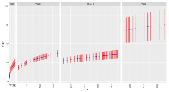
Figure 4. $\widehat{MTB{F}_t}$ and $95\%$ confidence intervals at the failure points. Red lines represent the range of the $95\%$ confidence intervals.

Table 5. Estimations for MTBF and their $95\%$ confidence intervals.

Type	MTBF	Lower Bound	$95\%$ Upper Bound
$X(t)$	90.851	66.7379	114.9641
$X(t)=0$	109.4868	74.4374	144.5362
$X(t)=1$	67.5841	55.5149	79.6534
$X(t)=2$	41.7184	33.5359	49.9009

In the model, the stress intensity of the experimental environment is reflected by the covariate scored by experts. An alternative method is to treat the stress intensity as a latent variable and incorporate it into $\mathit{\beta }$. In this case, we can set $\mathit{X}(t)$ as a 2-dimensional dummy variable, that is,

$$\mathit{X}(t)=\left\{\begin{array}{c}{(1,0)}^T,t\in [230,1687)\hfill \\ {(0,1)}^T,t\in [1687,3764)\hfill \\ {(0,0)}^T,others.\hfill \end{array}\right.$$

(34)

With the set of $\mathit{X}(t)$, the values of ${\mathit{\beta }}_1$ and ${\mathit{\beta }}_2$ in the coefficient vector represent the environmental stress intensity of Phases 2 and 3 during the test, respectively. The estimation results for the alternative model are shown in Table 6. It is shown that the stress intensity of Phase 3, ${\mathit{\beta }}_2$, is the highest, which is in line with the expert score. Note that ${\mathit{\beta }}_1$ is close to 0; we use the likelihood ratio test (33) to check whether ${\mathit{\beta }}_1=0$. The test statistic $-2logLR$ takes the value $0.0328$, which is less than the 95th percentile of ${\chi }_1^2$. So, the null hypothesis of ${\mathit{\beta }}_1=0$ cannot be rejected. The hypothesis test result fails to correspond to the actual setting of the test, where the environmental stress of Phase 2 is significantly stronger than that of the normal case. The increase in the number of parameters and the absence of experimental information render the model more susceptible to data fluctuations, which leads to greater estimation variance and insignificant estimation results. In future tests, this can be improved by increasing the length of testing time and collecting more monitoring information on the sensitive parameters of the tested engine.

Table 6. Estimation results.

Parameter	Estimation	Standard Deviation
$\gamma$	0.4486	0.2595
$\alpha$	0.6295	0.0681
${\mathit{\beta }}_1$	0.0435	0.2416
${\mathit{\beta }}_2$	0.6042	0.2368

7. Discussion

In this paper, we investigate an extension of the AMSAA model where the influence of the environment is considered as a time-dependent covariate vector. The covariate effects are incorporated into the AMSAA model as a proportional factor in the intensity function. To estimate the parameters in the NHPP-based model, the maximum likelihood estimation method is adopted. The properties of MLE, including existence, uniqueness, consistency, and asymptotic normality, are proved with several martingale properties of the designed counting process. Based on the MLE properties, the confidence interval estimation of the reliability measurement, mean time between failures, is deduced by the delta method. Moreover, a likelihood ratio test is designed to test whether any covariates influence the reliability growth process significantly. We verify the property and the efficiency of the proposed model in the simulation study, where a comparison is made with the classical AMSAA model. The results of the simulation demonstrate the necessity of taking covariate effects into account. A case study is conducted on the data collected from a multi-phase reliability growth test. We illustrate the practical use of the model by estimating the parameters and the MTBFs for the testing machine.

The proposed model is formulated based on the AMSAA model, in which failures are modeled by an NHPP whose intensity function corresponds to the power law. Nevertheless, the modeling approach and the proofs of its properties can be applied to NHPP models with an exponential family intensity function, which enables our model to be readily extended to these models. Furthermore, the covariate effects can be incorporated into the reliability growth model in more generalized forms in future work. As for application, our model can play an essential role in the design and planning of future reliability growth experiments, especially multi-stage reliability experiments.

References

- Li, M.; Xu, D.; Li, Z.S. A joint modeling approach for reliability growth planning considering product life cycle cost performance. Comput. Ind. Eng. 2020, 145, 106541. [Google Scholar] [CrossRef]
- Duane, J.T. Learning Curve Approach to Reliability Monitoring. IEEE Trans. Aerosp. 1964, 2, 563–566. [Google Scholar] [CrossRef]
- Crow, L.H. Reliability Analysis for Complex, Repairable Systems. In Reliability and Biometry; Proschan, F., Serfling, R.G., Eds.; SIAM: Philadelphia, PA, USA, 1974; pp. 379–410. [Google Scholar]
- Rigdon, S.E.; Basu, A.P. The Power Law Process: A Model for the Reliability of Repairable Systems. J. Qual. Technol. 1989, 21, 251–260. [Google Scholar] [CrossRef]
- Guo, H.; Zhao, W.W.; Mettas, A. Practical methods for modeling repairable systems with time trends and repair effects. RAMS ’06. Annu. Reliab. Maintainab. Symp. 2006, 2006, 182–188. [Google Scholar] [CrossRef]
- Taghipour, S.; Banjevic, D. Trend analysis of the power law process using Expectation–Maximization algorithm for data censored by inspection intervals. Reliab. Eng. Syst. Saf. 2011, 96, 1340–1348. [Google Scholar] [CrossRef]
- Tang, Z.; Zhou, W.; Zhao, J.; Wang, D.; Zhang, L.; Liu, H.; Yang, Y.; Zhou, C. Comparison of the Weibull and the Crow-AMSAA Model in Prediction of Early Cable Joint Failures. IEEE Trans. Power Deliv. 2015, 30, 2410–2418. [Google Scholar] [CrossRef]
- Li, D.; Tao, Y. Reliability Analysis of Emulsion Pump Based on Fault Tree and AMSAA Model. In Proceedings of the 2019 International Conference on Quality, Reliability, Risk, Maintenance, and Safety Engineering (QR2MSE), Zhangjiajie, China, 6–9 August 2019; pp. 545–550. [Google Scholar] [CrossRef]
- Coetzee, J.L. The role of NHPP models in the practical analysis of maintenance failure data. Reliab. Eng. Syst. Saf. 1997, 56, 161–168. [Google Scholar] [CrossRef]
- Lee, S.; Wilson, J.R.; Crawford, M.M. Modeling and simulation of a nonhomogeneous poisson process having cyclic behavior. Commun. Stat. Simul. Comput. 1991, 20, 777–809. [Google Scholar] [CrossRef]
- Gaudoin, O.; Yang, B.; Xie, M. Confidence Intervals for the Scale Parameter of the Power-Law Process. Commun. Stat. Theory Methods 2006, 35, 1525–1538. [Google Scholar] [CrossRef]
- Wang, B.X.; Xie, M.; Zhou, J.X. Generalized Confidence Interval for the Scale Parameter of the Power-Law Process. Commun. Stat. Theory Methods 2013, 42, 898–906. [Google Scholar] [CrossRef]
- Muralidharan, K.; Shah, R.; Dhandhukia, D.H. Future Reliability Estimation Based on Predictive Distribution in Power Law Process. Qual. Technol. Quant. M. 2008, 5, 193–201. [Google Scholar] [CrossRef]
- Di Crescenzo, A.; Martinucci, B. On a First-Passage-Time Problem for the Compound Power-Law Process. Stoch. Models 2009, 25, 420–435. [Google Scholar] [CrossRef]
- Oliveira, M.D.D.; Colosimo, E.A.; Gilardoni, G.L. Power Law Selection Model for Repairable Systems. Commun. Stat. Theory Methods 2013, 42, 570–578. [Google Scholar] [CrossRef]
- Zhao, J.; Wang, J. A New Goodness-of-Fit Test Based on the Laplace Statistic for a Large Class of NHPP Models. Commun. Stat. Simul. Comput. 2005, 34, 725–736. [Google Scholar] [CrossRef]
- Somboonsavatdee, A.; Sen, A. Statistical Inference for Power-Law Process with Competing Risks. Technometrics 2015, 57, 112–122. [Google Scholar] [CrossRef]
- Peng, Y.; Wang, Y.; Zi, Y.; Tsui, K.L.; Zhang, C. Dynamic reliability assessment and prediction for repairable systems with interval-censored data. Reliab. Eng. Syst. Saf. 2017, 159, 301–309. [Google Scholar] [CrossRef]
- Hu, J.M.; Huang, H.Z.; Li, Y.F. Reliability growth planning based on information gap decision theory. Mech. Syst. Signal Process. 2019, 133, 106274. [Google Scholar] [CrossRef]
- Van Dyck, J.; Verdonck, T. Precision of power-law NHPP estimates for multiple systems with known failure rate scaling. Reliab. Eng. Syst. Saf. 2014, 126, 143–152. [Google Scholar] [CrossRef]
- Slimacek, V.; Lindqvist, B.H. Nonhomogeneous Poisson process with nonparametric frailty and covariates. Reliab. Eng. Syst. Saf. 2017, 167, 75–83. [Google Scholar] [CrossRef]
- Barabadi, A.; Barabady, J.; Markeset, T. Application of reliability models with covariates in spare part prediction and optimization–A case study. Reliab. Eng. Syst. Saf. 2014, 123, 1–7. [Google Scholar] [CrossRef]
- Fleming, T.R.; Harrington, D.P. Counting Processes and Survival Analysis; John Wiley & Sons: Hoboken, NJ, USA, 2011; Volume 169. [Google Scholar]
- Wei, B.C. Exponential Family Nonlinear Models; Springer: Berlin/Heidelberg, Germany, 1998; Volume 1. [Google Scholar]
- Liptser, R. A strong law of large numbers for local martingales. Stochastics 1980, 3, 217–228. [Google Scholar] [CrossRef]
- Barndorff-Nielsen, O.E.; Sørensen, M. A review of some aspects of asymptotic likelihood theory for stochastic processes. Int. Stat. Rev. Int. Stat. 1994, 133–165. [Google Scholar] [CrossRef]
- Lewis, P.A.W.; Shedler, G.S. Simulation of nonhomogeneous poisson processes by thinning. Nav. Res. Logist. Q. 1979, 26, 403–413. [Google Scholar] [CrossRef]
Publisher’s Note: MDPI stays neutral with regard to jurisdictional claims in published maps and institutional affiliations. |
© 2021 by the authors. Licensee MDPI, Basel, Switzerland. This article is an open access article distributed under the terms and conditions of the Creative Commons Attribution (CC BY) license (https://creativecommons.org/licenses/by/4.0/).