On New Means with Interesting Practical Applications: Generalized Power Means

Abstract

Means of positive numbers appear in many applications and have been a traditional matter of study. In this work, we focus on defining a new mean of two positive values with some properties which are essential in applications, ranging from subdivision and multiresolution schemes to the numerical solution of conservation laws. In particular, three main properties are crucial—in essence, the ideas of these properties are roughly the following: to stay close to the minimum of the two values when the two arguments are far away from each other, to be quite similar to the arithmetic mean of the two values when they are similar and to satisfy a Lipchitz condition. We present new means with these properties and improve upon the results obtained with other means, in the sense that they give sharper theoretical constants that are closer to the results obtained in practical examples. This has an immediate correspondence in several applications, as can be observed in the section devoted to a particular example.

1. Introduction

Our experience with the application of means to several problems comes from the study of the numerical solution of conservation laws. In particular, in [1], a new limiter based on the $powe{r}_p$ mean was presented, giving rise to very efficient new methods of solving these kind of equations. This mean has the following expression:

$$powe{r}_p(x,y)=\frac{x+y}{2}(1-|\frac{x-y}{x+y}{|}^p),\mathrm{for}p\ge 1.$$

(1)

To our knowledge, this was the first time in the literature regarding the numerical solution of conservation laws that a new limiter was presented satisfying the following criteria:

• If $x=O\left(1\right)$, $y=O\left(1\right)$ and $|x-y|=O\left(h\right)$, then $|powe{r}_p(x,y)-\frac{x+y}{2}|=O\left(h^p\right).$
  This property is crucial to preserve the order of approximation of the methods in areas of regularity;
• $|powe{r}_p(x,y)|\le pmin\left\{\right|x|,|y\left|\right\}.$
  In applications, this property implies adaption in the case of discontinuities.

The case $p=2$ of these means coincides with the harmonic mean. These means were also used successfully in nonlinear subdivision and multiresolution schemes [2,3,4]. In this field of application, it is also quite important for the mean to satisfy the Lipchitz condition; in fact, the harmonic mean satisfies this prerequisite, as do the $powe{r}_p$ means, but the Lipchitz constant p is unfortunately larger than desirable to make theory and practice workable for higher-order methods.

In [5], the authors present a rigorous study of some specific typse of subdivision schemes, depending on a general mean $M(x,y)$. They propose the generalized means in the article as a particular example

$$G{M}_k(x_1,x_2):=\sqrt[k]{\frac{2x_1^k{x}_2^k}{x_1^k+x_2^k}}.$$

(2)

For these means, the required properties listed above are satisfied, and the Lipchitz constant is in these cases $\sqrt[k]{2}$ for $k\ge 1.$ This constant tends to 1 when k increases, and this is enough to allow for improvements in the theory and applications of nonlinear subdivision and multiresolution schemes, as well as in the numerical solution of conservation laws.

These means attain only two orders of approximation to the arithmetic mean in smooth areas. However, of course, one could immediately consider using the ideas introduced in [1] to generalize them to have p orders of approximation. Intuitively, the right candidate would be

$$G{M}_{k,p}(x_1,x_2):=\sqrt[k]{\frac{x^k+y^k}{2}(1-|\frac{x^k-y^k}{x^k+y^k}{|}^p)}.$$

(3)

Unfortunately, this is not the case, and the $G{M}_{k,p}$ means attain only two orders of approximation to the arithmetic mean in the sense described above. This fact can be taken from the observation $|\sqrt[k]{\frac{x^k+y^k}{2}}-\frac{x+y}{2}|=O\left(h^2\right)$ for whichever $k\ge 1.$

From this point on, one can try slight modifications of the given expression to find useful means that satisfy the mentioned properties with appropriate Lipchitz constants and allow high orders of approximation to be maintained. To our knowledge, there is no family of means with adaptivity constants tending to $1,$ with Lipchitz constant that also approach $1,$ and satisfy the requirement of proximity $O\left(h^p\right)$ to the arithmetic mean. Of course, one needs to be aware of proving each one of the properties carefully to ensure some basic properties are not lost while proving new ones. It is in this process that we have found an adequate expression, which opens up a variety of potential applications.

This work is organized as follows: in Section 2, we introduce the new mean and verify the most basic properties; in Section 3, we give the main results of the paper regarding the boundedness of the mean by a constant times the minimum of the two values, the approximation order to the arithmetic mean, and the Lipchitz condition; and finally, in Section 5, we show in some detail why this new mean is important for several applications, and we give some conclusions and perspectives for future work.

2. The Generalized Power Means

In this section, we introduce the proposed new family of means and prove some basic properties. Let us suppose $x>0$ and $y>0$; we define $G{P}_{k,p}$ for a natural number k and a real number $p\ge 1$ in the following way:

$$G{P}_{k,p}(x,y):=\sqrt[k]{{\left(\frac{x+y}{2}\right)}^k(1-|\frac{(x-y)g(x,y)}{{(x+y)}^k}{|}^p\left)\right)},$$

(4)

where $g(x,y)$ is a polynomial of degree $k-1$ defined by

$$g(x,y)=\left\{\begin{array}{cc}\sum _{j=0}^{k-1}(\sum _{i=0}^j(\genfrac{}{}{0pt}{}{k}{i}))x^j{y}^{k-1-j}\hfill & \mathrm{if}x\le y,\hfill \\ \sum _{j=0}^{k-1}(\sum _{i=0}^j(\genfrac{}{}{0pt}{}{k}{i}))y^j{x}^{k-1-j}\hfill & \mathrm{otherwise}.\hfill \end{array}\right.$$

(5)

Lemma 1.

Let us consider the function $r(x,y):=|\frac{(x-y)g(x,y)}{{(x+y)}^k}|$ for $x>0$ and $y>0$, and let us suppose that $x<=y$; then,

• $1-r=\frac{2^k{x}^k}{{(x+y)}^k},$
• $0\le r<1,$
• $r_x=\frac{-k{2}^k{x}^{k-1}y}{{(x+y)}^{k+1}},$
• $r_y=\frac{k{2}^k{x}^k}{{(x+y)}^{k+1}}.$

Proof. 

Let us start by proving the first point.

$$\begin{array}{ccc}\hfill 1-r& =& 1-\frac{(y-x)g(x,y)}{{(x+y)}^k}=\frac{{(x+y)}^k-(y-x)g(x,y)}{{(x+y)}^k}\hfill \\ & =& \frac{(1+{\sum }_{i=0}^{k-1}(\genfrac{}{}{0pt}{}{k}{i}))x^k}{{(x+y)}^k}=\frac{{\sum }_{i=0}^k(\genfrac{}{}{0pt}{}{k}{i})x^k}{{(x+y)}^k}\hfill \\ & =& \frac{2^k{x}^k}{{(x+y)}^k}.\hfill \end{array}$$

For the second point, it is apparent that $r\ge 0,$ and for the other inequality, we compute

$$\begin{array}{ccc}\hfill r& =& \frac{(y-x){\sum }_{j=0}^{k-1}({\sum }_{i=0}^j(\genfrac{}{}{0pt}{}{k}{i}))x^j{y}^{k-1-j}}{{(x+y)}^k}\hfill \\ & =& \frac{{\sum }_{j=0}^{k-1}({\sum }_{i=0}^j(\genfrac{}{}{0pt}{}{k}{i}))x^j{y}^{k-j}-{\sum }_{j=0}^{k-1}({\sum }_{i=0}^j(\genfrac{}{}{0pt}{}{k}{i}))x^{j+1}{y}^{k-1-j}}{{(x+y)}^k}\hfill \\ & =& \frac{y^k+{\sum }_{j=1}^{k-1}({\sum }_{i=0}^j(\genfrac{}{}{0pt}{}{k}{i}))x^j{y}^{k-j}-{\sum }_{j=1}^{k-1}({\sum }_{i=0}^{j-1}(\genfrac{}{}{0pt}{}{k}{i}))x^j{y}^{k-j}-({\sum }_{i=0}^{k-1}(\genfrac{}{}{0pt}{}{k}{i}))x^k}{{(x+y)}^k}\hfill \\ & =& \frac{{\sum }_{j=0}^{k-1}(\genfrac{}{}{0pt}{}{k}{j})x^j{y}^{k-j}-(2^k-1)x^k}{{\sum }_{j=0}^k(\genfrac{}{}{0pt}{}{k}{j})x^j{y}^{k-j}}.\hfill \end{array}$$

Now, taking into account the fact that ${\sum }_{j=0}^{k-1}(\genfrac{}{}{0pt}{}{k}{j})x^j{y}^{k-j}\ge (2^k-1)x^k,$ since $x\le y,$

$$r\le \frac{{\sum }_{j=0}^{k-1}(\genfrac{}{}{0pt}{}{k}{j})x^j{y}^{k-j}}{{\sum }_{j=0}^k(\genfrac{}{}{0pt}{}{k}{j})x^j{y}^{k-j}}<1.$$

The third point requires more computation. We start with the expression of the partial derivative with respect to x by applying simple derivation rules:

$$\begin{array}{ccc}\hfill r_x& =& \frac{(-g+(y-x)g_x)q-(y-x)g{q}_x}{q^2}\hfill \\ \hfill & =& \frac{-gq+y{g}_{x}q-x{g}_{x}q-yg{q}_x+xg{q}_x}{q^2},\hfill \end{array}$$

(6)

where q stands for the denominator in the quotient of polynomials $r(x,y).$

In view of Equation (6), we need to compute $g_x$ and $q_x$:

$$\begin{array}{ccc}\hfill g_x& =& \sum _{j=0}^{k-2}(j+1)(\sum _{i=0}^{j+1}\left(\genfrac{}{}{0pt}{}{k}{i}\right))x^j{y}^{k-2-j},\hfill \end{array}$$

(7)

$$\begin{array}{ccc}\hfill q_x& =& \sum _{j=0}^{k-1}\left(\genfrac{}{}{0pt}{}{k}{j+1}\right)x^j{y}^{k-2-j}.\hfill \end{array}$$

(8)

Now, we expand each product of polynomials in Equation (6); that is,

$$\begin{array}{ccc}\hfill -gq& =& -\sum _{j=0}^k\sum _{s=0}^{k-1}\left(\genfrac{}{}{0pt}{}{k}{j}\right)(\sum _{i=0}^s\left(\genfrac{}{}{0pt}{}{k}{i}\right))x^{j+s}{y}^{2k-1-j-s},\hfill \\ \hfill y{g}_{x}q& =& \sum _{j=0}^k\sum _{s=0}^{k-2}\left(\genfrac{}{}{0pt}{}{k}{j}\right)(s+1)(\sum _{i=0}^{s+1}\left(\genfrac{}{}{0pt}{}{k}{i}\right))x^{j+s}{y}^{2k-1-j-s},\hfill \\ \hfill -x{g}_{x}q& =& \sum _{j=0}^k\sum _{s=0}^{k-2}\left(\genfrac{}{}{0pt}{}{k}{j}\right)(s+1)(\sum _{i=0}^{s+1}\left(\genfrac{}{}{0pt}{}{k}{i}\right))x^{j+s+1}{y}^{2k-2-j-s},\hfill \\ \hfill -yg{q}_x& =& \sum _{j=0}^{k-1}\sum _{s=0}^{k-1}\left(\genfrac{}{}{0pt}{}{k}{j+1}\right)(j+1)(\sum _{i=0}^s\left(\genfrac{}{}{0pt}{}{k}{i}\right))x^{j+s}{y}^{2k-1-j-s},\hfill \\ \hfill xg{q}_x& =& \sum _{j=0}^{k-1}\sum _{s=0}^{k-1}\left(\genfrac{}{}{0pt}{}{k}{j+1}\right)(j+1)(\sum _{i=0}^s\left(\genfrac{}{}{0pt}{}{k}{i}\right))x^{j+s+1}{y}^{2k-2-j-s}.\hfill \end{array}$$

After extensive computations and applying the symmetry properties and basic results of combinatorial numbers, one can find that all coefficients are identically zero except the coefficient for $x^{k-1}y.$ Thus, finally, $r_x=\frac{-k{2}^k{x}^{k-1}y}{{(x+y)}^{k+1}}.$

The proof for $r_y$ is carried out following the same arguments. □

In the next result, we prove that $G{P}_{k,p}$ is in fact a mean of the two values x and y.

Theorem 1.

Let us consider $x>0$ and $y>0$; then,

$$min\{x,y\}\le G{P}_{k,p}(x,y)\le max\{x,y\}.$$

Proof. 

Let us suppose that $x\le y.$ We start by proving the first inequality $min\{x,y\}\le G{P}_{k,p}(x,y).$

$$\begin{array}{ccc}\hfill G{P}_{k,p}(x,y)& =& \sqrt[k]{{(\frac{x+y}{2})}^k(1-r^p)}\hfill \\ & =& \sqrt[k]{{(\frac{x+y}{2})}^k(1-r)(1+r+r^2+\dots +r^{p-1})}\hfill \\ & \ge & \sqrt[k]{{(\frac{x+y}{2})}^k(1-r)}\ge x,\hfill \end{array}$$

by using only the first point of Lemma 1.

Now, in order to prove the inequality $G{P}_{k,p}(x,y)\le max\{x,y\},$ we observe that since $0\le r<1$, this implies $0<1-r^p\le 1.$ Thus

$$\begin{array}{ccc}\hfill G{P}_{k,p}(x,y)& =& \sqrt[k]{{(\frac{x+y}{2})}^k(1-r^p)}\le \frac{x+y}{2}\le y.\hfill \end{array}$$

□

The relevance of these means is presented in the next section, in which we prove three main properties that have serious implications for the theoretical analysis of some numerical methods and also for their practical performance. They allow the definition of nonlinear methods by slightly modifying existing linear methods, generating adaptive counterparts that maintain the order of approximation (thanks to Proposition 2 in the next section), minimize the effect of discontinuities (as a consequence of Proposition 1) and retain the stability of the schemes (due to the possibility of obtaining contractive operators, due to the bound tending to 1 with the parameter k obtained in Proposition 3). For an explicit simple example, see Section 5.

3. Important Practical Properties of Generalized Power Means

In this section, we prove some specific properties that are essential for some applications, such as approximation theory, nonlinear subdivision and multiresolution schemes and the numerical solution of hyperbolic conservation laws. In particular, we consider the following: in the first result, we prove that the mean is bounded by a constant times the minimum argument; in the second result, we study the second-order approximation to the arithmetic mean; and in the third, we show that the mean satisfies a Lipchitz condition with an adequate constant.

Proposition 1.

Let us consider $x>0$ and $y>0$; then,

$$|G{P}_{k,p}(x,y)|\le \sqrt[k]{p}min\left\{\right|x|,|y\left|\right\}.$$

Proof. 

Let us suppose that $x\le y.$ Using the first point of Lemma 1, we can easily rewrite the expression of the proposed mean as $G{P}_{k,p}=x\sqrt[k]{1+r+r^2+\dots +r^{p-1}},$ and therefore, since according to the second point of Lemma 1 we have $r<1,$ we obtain the result. □

Proposition 2.

Let us consider $x>0$, $y>0.$ If $x=O\left(1\right)$, $y=O\left(1\right)$ and $|x-y|=O\left(h\right)$; then, $|G{P}_{k,p}(x,y)-\frac{x+y}{2}|=O\left(h^p\right).$

Proof. 

The proof begins with the following assertion:

$$|G{P}_{k,p}^k(x,y)-(\frac{x+y}{2}{)}^k|=(\frac{x+y}{2}{)}^k|\frac{(x-y)g(x,y)}{{(x+y)}^k}{|}^p=O(h^p).$$

Now, considering the function $g\left(x\right)=\sqrt[k]{x},$ defining $A=G{P}_{k,p}^k(x,y),$$B=(\frac{x+y}{2}{)}^k$ and applying the basic Lagrange theorem

$$|g(A)-g(B)|=|g^{\prime }(c)||B-A|=O(1)O(h^p)=O(h^p),\mathrm{where}c=O(1),c\in (A,B),$$

which completes the proof. □

Proposition 3.

Let us consider $\overline{x}>0$, $\overline{y}>0,$$\tilde{x}>0$ and $\tilde{y}>0$; then,

$$|G{P}_{k,p}(\overline{x},\overline{y})-G{P}_{k,p}(\tilde{x},\tilde{y})|\le Cmax\{|\overline{x}-\tilde{x}|,|\overline{y}-\tilde{y}\left|\right\},$$

where $C=\sqrt[k]{G_{p-1}}<\sqrt[k]{p},$ with $G_{p-1}:=1+r+r^2+\dots +r^{p-1}.$

Proof. 

Applying the mean value theorem, we obtain

$$|G{P}_{k,p}(\overline{x},\overline{y})-G{P}_{k,p}(\tilde{x},\tilde{y})|\le \underset{x,y}{max}\left|\right|\nabla G{P}_{k,p}(x,y){\left|\right|}_{1}max\left\{\right|\overline{x}-\tilde{x}|,|\overline{y}-\tilde{y}\left|\right\},$$

(9)

where $\left|\right|\nabla G{P}_{k,p}{(x,y)\left|\right|}_1=|\frac{\partial G{P}_{k,p}}{\partial x}|+|\frac{\partial G{P}_{k,p}}{\partial y}|.$

From the expression $G{P}_{k,p}(x,y)=x\sqrt[k]{1+r+\dots +r^{p-1}}$, computing $\frac{\partial G{P}_{k,p}}{\partial x}$ and $\frac{\partial G{P}_{k,p}}{\partial y}$, we obtain

$$\begin{array}{ccc}\hfill \frac{\partial G{P}_{k,p}}{\partial x}& =& \sqrt[k]{G_{p-1}}+\frac{1}{k}x{G}_{p-1}^{\frac{1}{k}-1}{r}_x{S}_{p-2},\hfill \end{array}$$

(10)

$$\begin{array}{ccc}\hfill \frac{\partial G{P}_{k,p}}{\partial x}& =& \frac{1}{k}x{G}_{p-1}^{\frac{1}{k}-1}{r}_y{S}_{p-2},\hfill \end{array}$$

(11)

with $G_{p-1}=1+r+r^2+\dots +r^{p-1},$ and $S_{p-2}=1+2r+3r^2+\dots +(p-1)r^{p-2}.$ Plugging into $\left|\right|\nabla G{P}_{k,p}(x,y){\left|\right|}_1$ the computations of $r_x$ and $r_y$ conducted in points 3 and 4 of Lemma 1, we obtain

$$\begin{array}{ccc}\hfill |\frac{\partial G{P}_{k,p}}{\partial x}|+|\frac{\partial G{P}_{k,p}}{\partial y}|& =& \sqrt[k]{G_{p-1}}+\sqrt[k]{G_{p-1}}\frac{2^k{x}^k}{{(x+y)}^{k+1}}\frac{S_{p-2}}{G_{p-1}}(x-y)\le \sqrt[k]{G_{p-1}},\hfill \end{array}$$

and this completes the proof with $C=\sqrt[k]{G_{p-1}}.$ □

4. Example of Application

The new means are well adapted to applications in some fields, such as nonlinear reconstruction operators, subdivision and multiresolution schemes. Our example is focused on a particular application to nonlinear subdivision schemes, although many other applications could be considered by simply improving some theoretical results that appear in articles that involve nonlinear means, such as the harmonic mean [1,4,6]. The reason for this lies in Propositions 1–3. Proposition 3, for instance, allows us to prove the stability of the scheme that we define in the following lines.

Given a set of nested grids in $[0,1]$:

$$X^s={\left\{x_j^s\right\}}_{j=0}^{J_s},x_j^s=j{h}_s,h_s=2^{-s}/J_0,J_s=2^s{J}_0,$$

where $J_0$ is some fixed integer, we consider the point-values $f_j^0=f(x_j^0)$ of a function $f\left(x\right)$ at the coarsest grid $X^0.$ Then, we refine the given data to finer scales according to the following definition of a subdivision scheme. First, let us introduce the second-order divided differences $D{f}_j^s:=\frac{f_{j-1}^s-2f_j^s+f_{j+1}^s}{2h_s^2},$ that, since we are working in uniform grids, relate to the second-order finite differences $\mathsf{\Delta }{f}_j=f_{j-1}^s-2f_j^s+f_{j+1}^s$ that appear at the numerator. Given this definition, and the data at a scale s over the grid $X^s,$ we consider one step of the subdivision scheme given by

$$f^{s+1}=S{f}^s=\left\{\begin{array}{cc}{f}_{2j}^{s+1}=f_j^s,\hfill & j=0,\dots ,J_s,\hfill \\ f_1^{s+1}=\frac{15}{48}{f}_0^s+\frac{45}{48}{f}_1^s-\frac{15}{48}{f}_2^s+\frac{3}{48}{f}_3^s,\hfill & j=0,\hfill \\ f_{2j+1}^{s+1}=\frac{f_j^s+f_{j+1}^s}{2}-\frac{h_s^2}{4}M(D{f}_j^s,D{f}_{j+1}^s),\hfill & j=1,\dots ,J_s-2,\hfill \\ f_{J_{s+1}-1}^{s+1}=\frac{15}{48}{f}_{J_s}^s+\frac{45}{48}{f}_{J_s-1}^s-\frac{15}{48}{f}_{J_s-2}^s+\frac{3}{48}{f}_{J_s-3}^s,\hfill & j=J_s-1,\hfill \end{array}\right.$$

(12)

where $M(x,y)$ stands for any mean of the values x and $y.$ Let us extend the definition of our mean $G{P}_{k,p},$ so that it can be used with both negative and positive values:

$${\widetilde{GP}}_{k,p}(x,y)=\left\{\begin{array}{cc}G{P}_{k,p}(x,y)\hfill & \mathrm{if}x>0,y>0,\hfill \\ -G{P}_{k,p}(-x,-y)\hfill & \mathrm{if}x<0,y<0,\hfill \\ 0\hfill & \mathrm{otherwise}.\hfill \end{array}\right.$$

(13)

For the sake of simplicity, $G{P}_{k,p}$ is referred to as the new extension below. We now consider the three following cases:

• $L(x,y)=\frac{x+y}{2},$ which gives the well known scheme of Deslauriers and Dubuc (DD) [7];
• $H(x,y)=\frac{2xy}{x+y},$ which defines the PPH subdivision scheme [3];
• $G{P}_{k,2}(x,y),$ given in Equation (4) with $p=2.$

We have chosen $p=2$ in the expression of the mean $G{P}_{k,p}$ in order to maintain the fourth-order approximation of the scheme in areas where the data come from smooth functions. In fact, if we take into account that the original scheme of Deslauriers and Dubuc [7] is known to be fourth-order accurate, which results from its definition using fourth-order piecewise centered Lagrange interpolation, we can also prove that the scheme based on $G{P}_{k,2}$ is fourth-order accurate. The key issue for this fact to be true is the use of Proposition 2 in order to see that if $f_{2j+1}^{s+1}$ stands for the DD subdivision at the intermediate points with odd indexes, ${\tilde{f}}_{2j+1}^{s+1}$ for the PPH subdivision and ${\widehat{f}}_{2j+1}^{s+1}$ for the generalized power means (GP) subdivision, we have

$$\begin{array}{ccc}\hfill |f_{2j+1}^{s+1}-{\tilde{f}}_{2j+1}^{s+1}|& \le & \frac{h_s^2}{4}|L(D{f}_j^s,D{f}_{j+1}^s)-H(D{f}_j^s,D{f}_{j+1}^s)|=O(h_s^4),\hfill \\ \hfill |f_{2j+1}^{s+1}-{\widehat{f}}_{2j+1}^{s+1}|& \le & \frac{h_s^2}{4}|L(D{f}_j^s,D{f}_{j+1}^s)-G{P}_{k,2}(D{f}_j^s,D{f}_{j+1}^s)|=O(h_s^4).\hfill \end{array}$$

We have chosen the values at the boundaries $f_1^{s+1}$ and $f_{J_{s+1}-1}^{s+1}$ by interpolating the first and last four data points using basic Lagrange interpolation. The nonlinear modifications then take place in the center of the intervals.

Remark 1.

In the expression for $f_{2j+1}^{s+1}$ in Equation (12), the dependence on the grid space $h_s$ is fictitious, as the expression can be rewritten by making use of the second-order finite differences as follows:

$$f_{2j+1}^{s+1}=\frac{f_j^s+f_{j+1}^s}{2}-\frac{1}{8}M(\mathsf{\Delta }{f}_j^s,\mathsf{\Delta }{f}_{j+1}^s),$$

which represents the way in which it is implemented in the computer programs.

It is important to notice that the second-order divided differences are indicators of the smoothness of the underlying function; in fact, the largest divided difference indicates the potential presence of a singularity in the data. Due to the boundedness of both the harmonic mean and the $G{P}_{k,p}$ means by a constant multiplied by the minimum of their two arguments (see Proposition 1), in the presence of a jump discontinuity in the data, the influence of a discontinuity in Equation (12) is limited. This behavior will occur for any nonlinear mean with this property. Let us suppose, for example, that a jump discontinuity lies in $[x_{j+1}^2,x_{j+2}^s]$; then, $D{f}_j=O(1),$$D{f}_{j+1}=O(\frac{1}{h^2}).$ However, $G{P}_{k,p}=O\left(1\right),$ and the contribution of the incorrect data $f_{j+2}^s$ to Equation (12) is neglected. Notice that, in this case, the order of approximation suffers a reduction to the second order, but it is not completely lost as in the case of the DD scheme, for example. With regard to practical properties in numerical examples, one expects similar behavior to existing nonlinear schemes based on the harmonic mean or some gain in adaption due to Proposition 1, which gives a smaller constant than the p-power means (generalizations of the harmonic mean) defined in [1], for example, for which we obtain p instead of $\sqrt[k]{p}$, which follows from Proposition 1 (see also the numerical experiments in Section 4 to observe the behavior of the schemes around the discontinuities).

Following the same idea presented in [3,6], it is possible to prove basic properties of the presented scheme for the mean $G{P}_{k,p}$, such as the existence of a nonlinear scheme $S_1$ for the first-order differences, the convergence of the subdivision scheme, the smoothness of the limit function of the subdivision scheme, the approximation order of the schemes, the behavior around jump discontinuities, the elimination of Gibbs effects and some other interesting properties. We focus on proving the stability of the subdivision scheme, which also shows the importance of Proposition 3. We first give the following simple lemma and a proposition regarding the contractivity of the finite difference operator.

Lemma 2.

The function $Z(x,y,z)$ defined in ${\mathbb{R}}^3$ by $Z(x,y,z)=\frac{x}{2}-\frac{1}{8}(G{P}_{k,2}(x,y)+G{P}_{k,2}(x,z))$ satisfies

• $\left|Z(x,y,z)\right|\le \frac{\left|x\right|}{2},$
• $sign\left(Z\right(x,y,z\left)\right)=sign\left(x\right),$
• $|Z(x,y,z)-Z(x^{\prime },y^{\prime },z^{\prime })|\le \frac{1}{2}|x-x^{\prime }|+\frac{\sqrt[k]{2}}{4}max\left\{\right|x-x^{\prime }|,|y-y^{\prime }|,|z-z^{\prime }\left|\right\}.$

Proof. 

Since $|G{P}_{k,2}(x,y)|\le \sqrt[k]{2}min\left\{\right|x|,|y\left|\right\}$ due to Proposition 1, we find that $|G{P}_{k,2}(x,y)|\le \sqrt[k]{2}\left|x\right|$ and $|G{P}_{k,2}(x,z)|\le \sqrt[k]{2}\left|x\right|.$ We also find that $sign\left(x\right)=sign\left(G{P}_{k,2}(x,y)\right)=sign\left(G{P}_{k,2}(x,z)\right),$ according to the extended definition of $G{P}_{k,2}$ given in (13). The combination of both arguments easily proves points 1 and 2.

In order to prove point 3, we use the triangular inequality and Proposition 3 as follows,

$$\begin{array}{ccc}\hfill |Z(x,y,z)-Z(x^{\prime },y^{\prime },z^{\prime })|& \le & \frac{1}{2}|x-x^{\prime }|+\frac{1}{8}|G{P}_{k,2}(x,y)-G{P}_{k,2}(x^{\prime },y^{\prime })|+\frac{1}{8}|G{P}_{k,2}(x,z)-G{P}_{k,2}(x^{\prime },z^{\prime })|\hfill \\ & \le & \frac{1}{2}|x-x^{\prime }|+\frac{\sqrt[k]{2}}{8}max\left\{\right|x-x^{\prime }|,|y-y^{\prime }\left|\right\}+\frac{\sqrt[k]{2}}{8}max\left\{\right|x-x^{\prime }|,|z-z^{\prime }\left|\right\}\hfill \\ & \le & \frac{1}{2}|x-x^{\prime }|+\frac{\sqrt[k]{2}}{4}max\left\{\right|x-x^{\prime }|,|y-y^{\prime }|,|z-z^{\prime }\left|\right\}.\hfill \end{array}$$

□

Proposition 4.

When removing s for simplicity, $\widehat{f}=S_{GP}f,$$\widehat{g}=S_{GP}g,$ where $S_{GP}$ stands for the subdivision scheme with the mean $G{P}_{k,2}$; then,

• $\left|\right|\mathsf{\Delta }\widehat{f}{\left|\right|}_{\infty }\le \frac{1}{2}{\left|\right|\mathsf{\Delta }f\left|\right|}_{\infty },$
• $\left|\right|\mathsf{\Delta }\widehat{f}-\mathsf{\Delta }\widehat{g}{\left|\right|}_{\infty }\le (\frac{1}{2}+\frac{\sqrt[k]{2}}{4})\left|\right|\mathsf{\Delta }f-{\mathsf{\Delta }g\left|\right|}_{\infty }.$

Proof. 

We first prove point 1; that is, for all indices $j,$

$$|\mathsf{\Delta }{\widehat{f}}_j|\le \frac{1}{2}{\left|\right|\mathsf{\Delta }f\left|\right|}_{\infty }.$$

We treat odd and even indices separately.

(a)

$j=2n+1.$

From (12) and (13), we find that

$$\begin{array}{ccc}\hfill {\widehat{f}}_{j-1}-2{\widehat{f}}_j+{\widehat{f}}_{j+1}& =& f_n-2{\widehat{f}}_j+f_{n+1}\hfill \\ & =& \frac{1}{8}G{P}_{k,2}(\mathsf{\Delta }{f}_n,\mathsf{\Delta }{f}_{n+1}),\hfill \end{array}$$

and thus, using Proposition 1

$$|\mathsf{\Delta }{\widehat{f}}_j|\le \frac{\sqrt[k]{2}}{8}min\left\{\right|\mathsf{\Delta }{f}_n|,|\mathsf{\Delta }{f}_{n+1}\left|\right\}\le \frac{\sqrt[k]{2}}{8}{\left|\right|\mathsf{\Delta }f\left|\right|}_{\infty }.$$

(b)

$j=2n.$ Again, from (12) and (13), we find that

$$\begin{array}{ccc}\hfill {\widehat{f}}_{j-1}-2{\widehat{f}}_j+{\widehat{f}}_{j+1}& =& {\widehat{f}}_{j-1}-2f_n+{\widehat{f}}_{j+1}\hfill \\ & =& Z(\mathsf{\Delta }{f}_n,\mathsf{\Delta }{f}_{n-1},\mathsf{\Delta }{f}_{n+1}).\hfill \end{array}$$

Thus, using Lemma 2, we obtain

$$|\mathsf{\Delta }{\widehat{f}}_j|\le \frac{|\mathsf{\Delta }{f}_n|}{2}\le \frac{1}{2}{\left|\right|\mathsf{\Delta }f\left|\right|}_{\infty },$$

which proves point 1.

In order to prove point 2, we again separate odd and even indices.

(a)

$j=2n+1.$

Using algebraic manipulations of the last point, we find that

$$\begin{array}{ccc}\hfill |\mathsf{\Delta }{\widehat{f}}_j-\mathsf{\Delta }{\widehat{g}}_j|& =& |{\widehat{f}}_{j-1}-2{\widehat{f}}_j+{\widehat{f}}_{j+1}-({\widehat{f}}_{j-1}-2{\widehat{f}}_j+{\widehat{f}}_{j+1})|\hfill \\ & =& \frac{1}{8}|G{P}_{k,2}(\mathsf{\Delta }{f}_n,\mathsf{\Delta }{f}_{n+1})-,G{P}_{k,2}(\mathsf{\Delta }{g}_n,\mathsf{\Delta }{g}_{n+1})|,\hfill \end{array}$$

and now, using Proposition 3, we obtain

$$|\mathsf{\Delta }{\widehat{f}}_j-\mathsf{\Delta }{\widehat{g}}_j|\le \frac{\sqrt[k]{2}}{8}\left|\right|\mathsf{\Delta }f-{\mathsf{\Delta }g\left|\right|}_{\infty }.$$

(b)

$j=2n.$ In this case, we can write

$$\begin{array}{ccc}\hfill |\mathsf{\Delta }{\widehat{f}}_j-\mathsf{\Delta }{\widehat{g}}_j|& =& |Z(\mathsf{\Delta }{f}_n,\mathsf{\Delta }{f}_{n-1},\mathsf{\Delta }{f}_{n+1})-Z(\mathsf{\Delta }{g}_n,\mathsf{\Delta }{g}_{n-1},\mathsf{\Delta }{g}_{n+1})|\hfill \\ & \le & \frac{1}{2}|\mathsf{\Delta }{f}_n-\mathsf{\Delta }{g}_n|+\frac{\sqrt[k]{2}}{4}max\{|\mathsf{\Delta }{f}_n-\mathsf{\Delta }{g}_n|,|\mathsf{\Delta }{f}_{n-1}-\mathsf{\Delta }{g}_{n-1}|,|\mathsf{\Delta }{f}_{n+1}-\mathsf{\Delta }{f}_{n+1}|\}\hfill \\ & \le & (\frac{1}{2}+\frac{\sqrt[k]{2}}{4})||\mathsf{\Delta }f-{\mathsf{\Delta }g||}_{\infty },\hfill \end{array}$$

by using point 3 of Lemma 2.

□

Remark 2.

If $k>1$ in Proposition 4, then the operator Δ is said to be contractive, and this fact is a crucial issue in the proof of the next theorem. Moreover, the smaller the contractivity constant, the better. Therefore, an increase in k gives a better constant. Thus, it could be proposed that the minimum of the two arguments should be used as the expression for the mean in (12), and this is optimal with regards to adaption, but at the cost of losing the approximation order given by Proposition 2, which would be no longer true. With the mean $G{P}_{k,2},$ we achieve both goals.

Let us now prove a theorem that ensures the stability of the subdivision scheme.

Theorem 2.

Given two initial sequences $f^0,g^0,$ let us consider $s+1$ steps of subdivision $f^{s+1}=S_{GP}\left(f^s\right),$$g^{s+1}=S_{GP}\left(g^s\right),$ where $S_{GP}$ stands for the subdivision scheme (12) with the mean $G{P}_{k,2},$ with $k>1$; then,

$$\left|\right|f^{s+1}-g^{s+1}{\left|\right|}_{\infty }\le C\left|\right|f^s-g^s{\left|\right|}_{\infty },$$

with $C=1+\frac{2\sqrt[k]{2}}{2-\sqrt[k]{2}}.$

Proof. 

Since $f^{s+1}=S_{GP}\left(f^s\right),$$g^{s+1}=S_{GP}\left(g^s\right),$ we can write

$$\begin{array}{ccc}\hfill f_{2j}^{s+1}& =& f_j^s,\hfill \\ \hfill g_{2j}^{s+1}& =& g_j^s,\hfill \\ \hfill f_{2j+1}^{s+1}& =& \frac{f_j^s+f_{j+1}^s}{2}-\frac{1}{8}G{P}_{k,2}(\mathsf{\Delta }{f}_j^s,\mathsf{\Delta }{f}_{j+1}^s),\hfill \\ \hfill g_{2j+1}^{s+1}& =& \frac{g_j^s+g_{j+1}^s}{2}-\frac{1}{8}G{P}_{k,2}(\mathsf{\Delta }{g}_j^s,\mathsf{\Delta }{g}_{j+1}^s).\hfill \end{array}$$

Therefore, we obtain

$$\begin{array}{ccc}\hfill |f_{2j}^{s+1}-g_{2j}^{s+1}|& =& |f_j^s-g_j^s|,\hfill \\ \hfill |f_{2j+1}^{s+1}-g_{2j+1}^{s+1}|& \le & \frac{|f_j^s-g_j^s|}{2}+\frac{|f_{j+1}^s-g_{j+1}^s|}{2}+\frac{1}{8}|G{P}_{k,2}(\mathsf{\Delta }{f}_j^s,\mathsf{\Delta }{f}_{j+1}^s)-G{P}_{k,2}(\mathsf{\Delta }{g}_j^s,\mathsf{\Delta }{g}_{j+1}^s)|.\hfill \end{array}$$

(14)

From (14), by using Proposition 3, we obtain

$$\begin{array}{ccc}\hfill \left|\right|f^{s+1}-g^{s+1}{\left|\right|}_{\infty }& \le & \left|\right|f^s-g^s{\left|\right|}_{\infty }+\frac{\sqrt[k]{2}}{8}\left|\right|\mathsf{\Delta }{f}^s-\mathsf{\Delta }{g}^s{\left|\right|}_{\infty }.\hfill \end{array}$$

Now, applying Proposition 4, we obtain

$$\begin{array}{ccc}\hfill \left|\right|f^{s+1}-g^{s+1}{\left|\right|}_{\infty }& \le & \left|\right|f^s-g^s{\left|\right|}_{\infty }+\frac{\sqrt[k]{2}}{8}{B}^s\left|\right|\mathsf{\Delta }{f}^0-\mathsf{\Delta }{g}^0{\left|\right|}_{\infty },\hfill \end{array}$$

(15)

with $B=\frac{1}{2}+\frac{\sqrt[k]{2}}{4}.$ Applying the same reduction as in (15) recursively, we reach

$$\left|\right|f^{s+1}-g^{s+1}{\left|\right|}_{\infty }\le \left|\right|f^0-g^0{\left|\right|}_{\infty }+\frac{\sqrt[k]{2}}{8}(\sum _{i=0}^s{B}^i)\left|\right|\mathsf{\Delta }{f}^0-\mathsf{\Delta }{g}^0{\left|\right|}_{\infty }.$$

Taking into account the fact that ${\sum }_{i=0}^s{B}^i=1+\frac{4}{2-\sqrt[k]{2}},$ and $\left|\right|\mathsf{\Delta }{f}^0-\mathsf{\Delta }{g}^0{\left|\right|}_{\infty }\le 4\left|\right|f^0-g^0{\left|\right|}_{\infty },$ we finally obtain

$$\left|\right|f^{s+1}-g^{s+1}{\left|\right|}_{\infty }\le C\left|\right|f^s-g^s{\left|\right|}_{\infty },$$

with $C=1+\frac{2\sqrt[k]{2}}{2-\sqrt[k]{2}}.$ □

Remark 3.

In [6], the authors prove a similar theorem for the PPH subdivision scheme following similar arguments, and a stability constant $C_{PPH}=9$ is obtained, which is larger than the value of $C=5.8284$ obtained from Theorem 2 for $k=2$ or $C=4.4048$ for $k=3.$ In the limit, when k grows to infinity, we obtain $C=3.$ The practical importance of having a smaller stability constant lies in the fact that, in order to ensure a prescribed tolerance ϵ in the final error, one can use approximated input data with $\frac{ϵ}{C}$ error. Therefore, there is more flexibility to ensure the required precision.

Numerical Test

Let us consider the function $f\left(x\right)$ defined in the interval $[0,1]$ and given by

$$f\left(x\right)=\left\{\begin{array}{cc}sin\left(2\pi x\right),\hfill & \mathrm{if}x\le \frac{1}{2},\hfill \\ -10-sin\left(2\pi x\right),\hfill & \mathrm{if}x>\frac{1}{2}.\hfill \end{array}\right.$$

(16)

We consider the set of initial data given by the point value discretization of the function $f\left(x\right)$ in 20 equally spaced points; that is, $f_i^0:=f\left(x_i\right),$$x_i=\frac{i}{19},$$i=0,\dots ,19.$ Our purpose is to see the result of applying linear and nonlinear subdivision schemes in the presence of a jump discontinuity and also to compare the approximation of the limit function with perturbed data $g^0$ and estimate the stability constant given in Theorem 2 simply by computing,

$$C=\frac{\left|\right|f^{s+1}-g^{s+1}{\left|\right|}_{\infty }}{\left|\right|f^s-g^s{\left|\right|}_{\infty }},$$

(17)

after $s+1=15$ levels of subdivision.

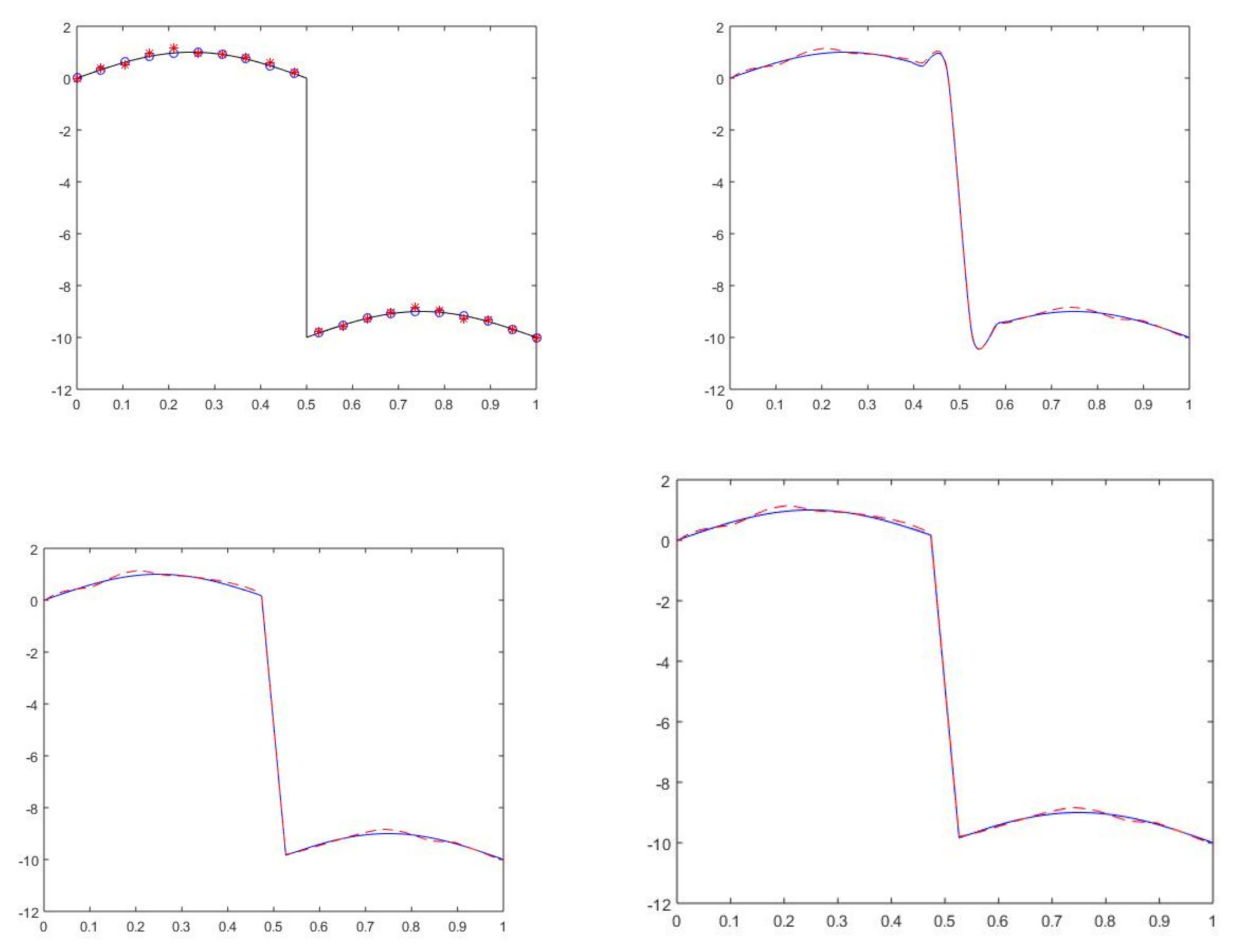
We have implemented random perturbations of the original data with the maximum absolute values $\lambda =0.1,$$\lambda =0.05$ and $\lambda =0.001.$ Then, we have computed the stability constant indicated in (17) for the three subdivision schemes considered; that is, $C_{DD},$ $C_{PPH}$ and $C_{GP}$, respectively. The obtained estimations are given in

Table 1. Estimations of the stability constant in Theorem 2 for the DD, PPH and GP subdivision schemes after 15 levels of subdivision.

$\mathit{\lambda }$	DD	PPH	${\mathit{GP}}_{2,2}$	${\mathit{GP}}_{3,2}$
$0.1$	$1.0393$	$1.0310$	$1.0205$	$1.0141$
$0.05$	$1.0011$	$1.0057$	$1.0047$	$1.0038$
$0.001$	$1.0184$	$1.0140$	$1.0103$	$1.0073$

. It can be seen that, in practice, the three methods behave in a very stable way, and that the stability constants are normally much smaller than the theoretical estimates. However, we want to point out that the bound given in Theorem 2 is sharper than the one obtained for the PPH method. We also see that the larger the k, the better the estimation and the adaption to the expected reproduction of the original function around the jump discontinuity. It is also interesting to observe how the nonlinear subdivision schemes define the area around the discontinuity better, while the linear counterpart generates undesirable effects in this zone; see Figure 1.

Remark 4.

The $G{P}_{k,p}$ means may require arithmetic with variable precision for larger values of k, and the computational time also grows considerably with k, which needs to be taken into account. Therefore, a balance between these points must be considered depending on the application. The theoretical simplicity of the proofs using this $G{P}_{k,p}$ in the schemes is undeniable, which in some cases may allow for theoretical results that are much more difficult or even not possible to obtain for other means—see, for example, the work presented in [4], where the authors do not reach any theoretical results regarding stability due to the difficulty of obtaining a contraction property for the finite differences, as achieved in Proposition 4 for the mean $G{P}_{k,2}.$

5. Conclusions and Perspectives

We have presented a new family of means. Some important applications require means that satisfy some remarkable properties that are achieved by this specific family, as has been theoretically proven. More precisely, we have shown that these means can be bounded by a constant times the minimum of the two arguments, with the possibility of choosing a member of the family with a constant that is larger than 1 but as close to 1 as needed. We have shown the existence of similar constants for the Lipchitz property. We have also proven a property regarding the approximation order p to the arithmetic mean.

We have commented about the possibility of applying the new means in several applications, and in particular, we have two main applications in mind: the first is to design high-order reconstruction methods allowing for stability theory, inner subdivision and multiresolution schemes, improving on the work of [4]; the second is the substitution of the power-p means for the generalized power means as limiters into the schemes in [1] for hyperbolic conservation laws. Finally, we have given a particular application as an example of how easy the theory becomes thanks to the nearer-unity constants given in the presented propositions. In this particular example, we can also observe the adaption properties attained by the presented subdivision scheme.

References

- Marquina, A.; Serna, S. Power ENO methods: A fifth-order accurate weighted power ENO method. J. Comput. Phys. 2004, 194, 632–658. [Google Scholar]
- Floater, M.S.; Micchelli, C.A. Nonlinear stationary subdivision. In Approximation Theory: In Memory of A.K. Varna; Govil, N.K., Mohapatra, N., Nashed, Z., Sharma, A., Szabados, J., Eds.; CRC Press: Boca Raton, FL, USA, 1998; pp. 209–224. [Google Scholar]
- Amat, S.; Donat, R.; Liandrat, J.; Trillo, J.C. Analysis of a new nonlinear subdivision scheme. Applications in image processing. Found. Comput. Math. 2006, 6, 193–225. [Google Scholar] [CrossRef]
- Amat, S.; Dadourian, K.; Liandrat, J.; Trillo, J.C. High order nonlinear interpolatory reconstruction operators and associated multiresolution schemes. J. Comput. Appl. Math. 2013, 253, 163–180. [Google Scholar] [CrossRef]
- Guessab, A.; Moncayo, M.; Schmeisser, G. A class of nonlinear four-point subdivision schemes. Adv. Comput. Math. 2012, 37, 151–190. [Google Scholar] [CrossRef]
- Amat, S.; Liandrat, J. On the stability of PPH nonlinear multiresolution. Appl. Comput. Harmon. Anal. 2005, 18, 198–206. [Google Scholar] [CrossRef] [Green Version]
- Deslauriers, G.; Dubuc, S. Symmetric Iterative Interpolation Scheme. Constr. Approx. 1989, 5, 49–68. [Google Scholar] [CrossRef]
Figure 1.
Limit functions obtained with 16 levels of subdivision from the original data and their perturbed version with a random perturbation of size (Top-left): Original function in black—initial data in blue circles and perturbed data in red asterisks. (Top-right): Subdivision using DD. (Bottom-left): Subdivision using PPH. (Bottom-right): Subdivision using with The subdivision for the original data is shown with the blue solid line, and that for the perturbed data with the red broken line.