Solving 3-D Gray–Scott Systems with Variable Diffusion Coefficients on Surfaces by Closest Point Method with RBF-FD

Abstract

The Gray–Scott (GS) model is a non-linear system of equations generally adopted to describe reaction–diffusion dynamics. In this paper, we discuss a numerical scheme for solving the GS system. The diffusion coefficients of the model are on surfaces and they depend on space and time. In this regard, we first adopt an implicit difference stepping method to semi-discretize the model in the time direction. Then, we implement a hybrid advanced meshless method for model discretization. In this way, we solve the GS problem with a radial basis function–finite difference (RBF-FD) algorithm combined with the closest point method (CPM). Moreover, we design a predictor–corrector algorithm to deal with the non-linear terms of this dynamic. In a practical example, we show the spot and stripe patterns with a given initial condition. Finally, we experimentally prove that the presented method provides benefits in terms of accuracy and performance for the GS system’s numerical solution.

1. Introduction

Reaction–diffusion systems model many physical phenomena. In fact, such a system is frequently encountered into many branches of physics, such as electromagnetism [1],  heat transfer [2], and diffusion [3]. For the problem of fluid mechanics in porous formations (aquifers and petroleum reservoirs), reaction–diffusion equations lend themselves as a powerful diagnostic tool to determine the hydraulic properties of formations. Briefly, from a well (or a battery of wells), the water is pumped/injected over a measured interval. The effect of such a stimulation upon the pressure distribution in the flow domain is recorded, and the hydraulic properties are detected by matching the measured pressure values against the theoretical ones.

In the context of hydrological applications, several analytical studies are focused on solving reaction–diffusion equations (see [4] for a comprehensive collection of the classical solutions). These analytical studies commonly model the formation as homogeneous (or at most as a sequence of homogeneous layers). However, geological formations are de facto heterogeneous with hydraulic conductivity, in particular, varying in the space somewhat largely (see, e.g., [5]). These irregular changes have a tremendous impact upon transport processes taking place in porous formations [6]. The common (and widely accepted) approach to tackle these erratic spatial variations is a stochastic framework that regards the conductivity as a random space function [7], therefore rendering the reaction–diffusion equation(s) stochastic [7]. Consequently, mean values are insufficient to adequately characterize the spatial distribution of the aquifer’s parameters (that now become random fields) since one is required to quantify the uncertainty. Hence, uncertainty quantification has witnessed developments in response to the promise of achieving reliable predictions. In this research field, the integration of ideas from multiple disciplines to effectively design actions is being adopted by engineers, mathematicians, physicists. Uncertainty of any random field $\Sigma$ can be quantified by deriving deterministic equations governing the probability density function of $\Sigma$ or, alternatively, by computing moments of $\Sigma$ [8]. Although quantifying the uncertainty of such random fields is a mathematically challenging problem, it has been scarcely considered in the past (partly due to technical difficulties).

In this paper, we consider one of the most interesting models in engineering, physics, and chemistry, the Gray–Scott (GS) system, which describes the following chemical reaction:

$$\left\{\begin{array}{c}U+2V⟶3V,\hfill \\ V⟶P,\hfill \end{array}\right.$$

(1)

where U, V, and P are chemicals. The corresponding GS surface model has the form

$$\begin{array}{c}\frac{\partial u(\mathbf{x},t)}{\partial t}={\nabla }_{\Gamma }.\left[D_u(\mathbf{x},t){\nabla }_{\Gamma }u(\mathbf{x},t)\right]-u(\mathbf{x},t)v^2(\mathbf{x},t)+F(1-u(\mathbf{x},t)),\mathbf{x}\in \Gamma \subset {\mathbb{R}}^3,t\ge 0,\hfill \\ \frac{\partial v(\mathbf{x},t)}{\partial t}={\nabla }_{\Gamma }.\left[D_v(\mathbf{x},t){\nabla }_{\Gamma }v(\mathbf{x},t)\right]+u(\mathbf{x},t)v^2(\mathbf{x},t)-(F+K)v(\mathbf{x},t),\mathbf{x}\in \Gamma \subset {\mathbb{R}}^3,t\ge 0,\hfill \end{array}$$

(2)

where $u(\mathbf{x},t)$ and $v(\mathbf{x},t)$ are the concentrations of chemical species; $D_u(\mathbf{x},t)$ and $D_v(\mathbf{x},t)$ are the variable diffusion coefficients of the chemicals species U and V, respectively; K is the conversion rate from U to P; and F is the in-flow rate of u from the outside; therefore $(F+K)$, is the removal rate of v from the reaction field; ${\nabla }_{\Gamma }$ denotes the curve gradient operator. We aim to design and implement a numerical method to solve (2) using a radial basis function combined with finite differences method (RBF-FD). This represents the first (but most important) step toward uncertainty quantification of the random fields u–v. However, in this work, a more general novel case is considered in which the system coefficients depend on space and time. For this reason, first, an implicit difference stepping method is adopted to semi-discretize the model in the time direction. Then, a hybrid advanced meshless approach is considered to fully discretize the model. In this way, an effective sparse meshless method based on radial basis function–finite difference (RBF-FD) technique combined with the closest point method (CPM), as an efficient embedding procedure for solving PDEs on surfaces, is proposed. Here, we suggest a predictor–corrector algorithm to deal with the non-linear terms of the dynamics. Finally, we prove through experiments that RFB-FD provides benefits in terms of accuracy and performance.

The paper is organized as follows: Section 2 provides a review of related works; Section 3 describes the numerical discretization procedure. In Section 4, some numerical experiments are considered.

2. Related Numerical Works

The so-called Turing models are coupled partial differential equations describing the reaction and diffusion behaviour of chemicals. The fundamental concept introduced by Turing was that diffusion favours model instability; as a consequence, these models describe the arising of spatially heterogeneous configurations [9]. These formations are called Turing patterns and were firstly observed in chemical experiments; then, they attracted the attention of mathematical biologists due to their ability to imitate biological both regular patterns, such as the stripes of a zebra or the spots of a cheetah, and more irregular patterns, such as those of leopards and giraffes. Moreover, branching in plants and spot patterns of vegetation in the deserted area are also described. As for vegetation dynamics, results concerning the numerical counterpart of the Turing instability have been investigated [10]. In the Gray–Scott model, the reactions create patterns that successfully describe formations in living things. Data on the intriguing history of the Gray–Scott reaction–diffusion model and its applications to the real world are freely available at Robert Munafo’s web page [11]. The main results concerning evidence of the Gray–Scott equations documented in the following: Turing 1952 (embryo gastrulation; multiple spots in a 1-D system), Bard and Lauder 1974 (leaves, hair follicles), Bard, 1981 (spots on deer and giraffe), Murray 1981 (butterfly wings), Meinhardt 1982 (stripes, veins on leaf), Young 1984 (development of eye), Meinhardt and Klinger 1987 (mollusk shells), Turk 1991 (leopard, jaguar, zebra). Reaction and diffusion of chemical species can produce a variety of patterns. These PDE systems model pattern formation on curved surfaces. Here, we present a numerical study for studying Turing patterns [12]. In our approach, we adopt a meshless scheme based on radial basis function–finite difference (RBF-FD). Moreover, we use the closest point discretization to deal with the computational complexity of the problem. Radial basis functions (RBFs) are a fundamental mesh-free method to numerically solve PDEs on irregular domains (see [13,14,15] for the global collocation approach). This is due to the versatility of scattered data interpolation techniques used in several applications, e.g., surface reconstruction, image restoration, and in painting, meshless/Lagrangian methods for fluid dynamics [16]. The numerical solution of elliptic partial differential equations by a global collocation approach based on RBF refers to a strong-form solution in the PDE literature [13].

The main drawback for the global approach, although spectrally accurate, consists of solving large, ill-conditioned, dense linear systems, and many attempts are known to deal with it [17,18]. In some cases, local methods are preferred, giving up spectral accuracy for a sparse, better-conditioned linear system and more flexibility for handling non-linearities. The comprehensive literature concerns local RBF schemes by partitioning the domain, referred to as partition of unity (PU) [19,20,21].

An open issue in RBF theory concerns the choice of the shape parameter. The study of this parameter is a crucial topic to guarantee the stability of numerical methods. To overcome the problem, hybrid approaches called variably scaled kernels (VSKs) have been recently introduced [22].

In [23], the authors propose a different local approach based on a generalization of the classical finite difference (FD) method. The FD weights are computed using polynomial interpolation [24,25]. Finite difference methods are applied to solve PDEs on triangulated surfaces [26]. Some numerical issues are involved in the geometric quantities calculation, including values of the normal vector or the curvature of a surface [27]. For solving PDEs on surfaces with complex geometries [28], a level set representation of surfaces and the use of smart projection operators are generally adopted. RBF approaches are also discussed in the literature for the sphere [29] and to deal with embedded surfaces [30,31].

Regarding the level set representation of a surface, the closest point represents a surface, whereby grid nodes store the closest point in Euclidean distance to the surface, successfully used in the computation of diffusion-generated motions of curves on surfaces [32]. The closest point operator is generally designed to solve PDEs on surfaces in embedding space to extend the problem from the surface to the surrounding space. This method allows for boundary conditions at surface boundaries and immediately generalizes beyond surfaces embedded in ${\mathbb{R}}^3$ to objects of any dimension embedded in any ${\mathbb{R}}^n$ [33].

The CPM is generally designed for problems posed on static surfaces [33], using standard finite difference schemes. The classical formulation adopts explicit time stepping, and the stability results are given in the surface case (see [34] for details). Finally, the solution of PDEs on moving surfaces is also of considerable interest. In this paper, we solve the GS system on surfaces by proposing an implicit formulation in the time direction. Moreover, the RBF-FD [35,36] is considered to discretize the time-independent problem in the spatial direction.

3. Numerical Discretization Scheme

Here, an accurate implicit formulation is proposed to discretize the problem (2) in the time direction. For this purpose, firstly, the time interval $[0,T]$ is uniformly decomposed into M sub-intervals ${\bigcup }_{j=0}^{M-1}[t^j,t^{j+1}]$, where $t^j=j\tau$, $j=0,\cdots ,M$ and $\tau =T/M$ is time step size. Then, by substituting $t=t^{n+1}$ in the system (2), the following relations are obtained:

$$\begin{array}{c}\frac{\partial u(\mathbf{x},t^{n+1})}{\partial t}={\nabla }_{\Gamma }·\left[D_u(\mathbf{x},t^{n+1}){\nabla }_{\Gamma }u(\mathbf{x},t^{n+1})\right]-u(\mathbf{x},t^{n+1})v^2(\mathbf{x},t^{n+1})+F(1-u(\mathbf{x},t^{n+1})),\hfill \\ \frac{\partial v(\mathbf{x},t^{n+1})}{\partial t}={\nabla }_{\Gamma }·\left[D_v(\mathbf{x},t^{n+1}){\nabla }_{\Gamma }v(\mathbf{x},t^{n+1})\right]+u(\mathbf{x},t^{n+1})v^2(\mathbf{x},t^{n+1})-(F+K)v(\mathbf{x},t^{n+1})\hfill \end{array}$$

(3)

with $\mathbf{x}\in \Gamma \subset {\mathbb{R}}^3$ and $t\in [0,T]$. The time integer derivative can be discretized at two sequential time levels, $n+1$ and n, as follows:

$$\frac{\partial u(\mathbf{x},t^{n+1})}{\partial t}=\frac{u^{n+1}-u^n}{\tau }+R^{n+1},\frac{\partial v(\mathbf{x},t^{n+1})}{\partial t}=\frac{v^{n+1}-v^n}{\tau }+R^{n+1},$$

(4)

where $u^n=u(\mathbf{x},t^n)$ and $v^n=v(\mathbf{x},t^n)$. In addition, $R^{n+1}$ denotes the truncation error that is bounded by $|R^{n+1}|<C\tau$. By substituting Equation (4) in (3), the following relations at the $(n+1)-$th time level for $n=0,1,2,\cdots ,M-1$ are obtained:

$$\begin{array}{c}\frac{u^{n+1}-u^n}{\tau }={\nabla }_{\Gamma }·\left(D_u^{n+1}{\nabla }_{\Gamma }{u}^{n+1}\right)-u^{n+1}{\left(v^{n+1}\right)}^2+F(1-u^{n+1})\hfill \\ \frac{v^{n+1}-v^n}{\tau }={\nabla }_{\Gamma }·\left(D_v^{n+1}{\nabla }_{\Gamma }{v}^{n+1}\right)+u^{n+1}{\left(v^{n+1}\right)}^2-(F+K)v^{n+1}.\hfill \end{array}$$

(5)

By rearranging the above relations, the following equations result in the following:

$$\begin{array}{c}(1+\tau F)u^{n+1}-\tau {\nabla }_{\Gamma }·\left(D_u^{n+1}{\nabla }_{\Gamma }{u}^{n+1}\right)=-\tau u^{n+1}{\left(v^{n+1}\right)}^2+\tau F+u^n,\hfill \\ (1+\tau (F+K))v^{n+1}-\tau {\nabla }_{\Gamma }·\left(D_v^{n+1}{\nabla }_{\Gamma }{v}^{n+1}\right)=\tau u^{n+1}{\left(v^{n+1}\right)}^2+v^n.\hfill \end{array}$$

(6)

Now, we consider the closest point method for solving PDEs on surfaces using the RBF-FD to discretize the time-independent problems (6) in the spatial direction. In the following subsection, we discuss space decomposition schemes.

3.1. Closest Point Method

CPM is an embedding approach for numerically solving partial differential equations on surfaces. It considers a limited, narrow band surrounding the surface $\Gamma$. Then, the closest point function maps each point of the embedding band to its closest point on the surface. CPM applies different standard numerical techniques to solve the embedding PDEs. Since it preserves the solution constant along with normal directions to the surface, the gradient and Laplacian over the embedding space all retrieve their inherent surface properties when restricted to the surface. The obtained embedding solutions are equal to the original PDEs’ solutions on the surface. In this work, an efficient local meshless method based on RBFs is combined with CPM.

We consider the surface $\Gamma \subset {\mathbb{R}}^d$ and $\mathbf{\xi }$ to be a point in the embedding space $\Omega \subset {\mathbb{R}}^d$. The closest point function for $\Gamma$ is defined by

$$C{P}_{\Gamma }\left(\xi \right)=arg\underset{\mathbf{x}\in \Gamma }{min}\parallel \mathbf{x}-\mathbf{\xi }\parallel ,$$

(7)

which identifies the closest point of $\mathbf{\xi }$ on the surface $\Gamma$.

In a neighborhood of the surface, $C{P}_{\Gamma }$ is $C^l$-smooth for a $C^{l+1}$-smooth surface $\Gamma$. Moreover, the embedding space $\Omega$ is considered a tubular neighborhood of surface $\Gamma$. To prevent the entry discontinuities into $C{P}_{\Gamma }$, it should be assumed that the radius of the computational tube, $\Omega$, has been chosen such that it consists only of points within a distance ${\kappa }_{\infty }^{-1}$ of the surface $\Gamma$, where ${\kappa }_{\infty }$ is an upper bound on the curvatures of $\Gamma$ [37].

Regarding the CPM, solving the surface PDE on the surface is converted to solving a proper embedding PDE on the computational domain; the surface derivatives should be replaced with Cartesian derivative and closest points operators according to two principles [33]:

• Suppose V to be a function defined on ${\mathbb{R}}^d$ that is constant along normal directions of $\Gamma$. Then, at the surface, ${\nabla }_{\Gamma }V=\nabla V$.
• Suppose $\mathbf{V}$ to be a vector field on ${\mathbb{R}}^d$ that is tangent to $\Gamma$ and also tangent at all surfaces displaced by a fixed distance from $\Gamma$. Then, at the surface, ${\nabla }_{\Gamma }·\mathbf{V}=\nabla ·\mathbf{V}$.

The first principle states that if a function is constant in the normal direction, it only varies along the surface. Moreover, the second principle explains that a flux that is directed everywhere along the surface can only spread out within the surface directions.

If u is a function defined on the surface, $u\left(CP\right)$ is constant along the directions normal to the surface; thus, the first principle implies

$${\nabla }_{\Gamma }u=\nabla u\left(CP\right).$$

(8)

Since $u\left(CP\right)$ is tangent to the distance function’s level-sets, applying the second principle yields the surface Laplacian, which is known as the Laplace–Beltrami operator in the following form:

$${\nabla }_{\Gamma }·\left({\nabla }_{\Gamma }u\right)=\nabla ·(\nabla u\left(CP\right)).$$

(9)

More generally, we consider the surface diffusion operator ${\nabla }_{\Gamma }·\left(A\left(\mathbf{x}\right){\nabla }_{\Gamma }\right)$, where the diffusion coefficient is not constant and depends on position. In this case, $A\left(CP\right)\nabla \left(u\right(CP\left)\right)$ is tangent to the level surfaces, which implies

$${\nabla }_{\Gamma }·\left(A\left(\mathbf{x}\right){\nabla }_{\Gamma }u\right)=\nabla ·(A\left(CP\right)\nabla \left(u\left(CP\right)\right)).$$

(10)

By combining the two principles, all surface differential operators in the governing problem can be replaced with the corresponding Cartesian differential operators. Therefore, by using the relation (10), the surface Equations (6) are changed to the embedding equations, which depend only on Cartesian derivatives as follows:

$$\begin{array}{c}(1+\tau F){\widehat{u}}^{n+1}-\tau \nabla ·(D_{\widehat{u}}^{n+1}\nabla {\widehat{u}}^{n+1})=-\tau {\widehat{u}}^{n+1}{\left({\widehat{v}}^{n+1}\right)}^2+\tau F+{\widehat{u}}^n,\hfill \\ (1+\tau (F+K)){\widehat{v}}^{n+1}-\tau ·(\nabla D_{\widehat{v}}^{n+1}\nabla {\widehat{v}}^{n+1})=\tau {\widehat{u}}^{n+1}{\left({\widehat{v}}^{n+1}\right)}^2+{\widehat{v}}^n.\hfill \end{array}$$

(11)

where the constants along the normal direction extension of u and v are denoted by  $\widehat{u}:\Omega \to \mathbb{R}$ and $\widehat{v}:\Omega \to \mathbb{R}$, respectively. The above relations are equivalent to

$$\begin{array}{c}(1+\tau F){\widehat{u}}^{n+1}-\tau \nabla D_{\widehat{u}}^{n+1}\nabla {\widehat{u}}^{n+1}-\tau D_{\widehat{u}}^{n+1}{\nabla }^2{\widehat{u}}^{n+1}=-\tau {\mathcal{G}}^{n+1}+\tau F+{\widehat{u}}^n,\hfill \\ (1+\tau (F+K)){\widehat{v}}^{n+1}-\tau \nabla D_{\widehat{v}}^{n+1}\nabla {\widehat{v}}^{n+1}-\tau D_{\widehat{v}}^{n+1}{\nabla }^2{\widehat{v}}^{n+1}=\tau {\mathcal{G}}^{n+1}+{\widehat{v}}^n,\hfill \end{array}$$

(12)

where ${\mathcal{G}}^{n+1}={\widehat{u}}^{n+1}{\left({\widehat{v}}^{n+1}\right)}^2$. Finally, the points are on the tubular computational domain, and the corresponding closest point on the surface forms the closest point representation. Therefore, a suitable platform was provided for performing a suitable numerical method in order to solve the embedding problem.

3.2. CPM Based on RBF-FD Technique

The radial basis function–finite difference (RBF-FD) method is a hybrid and advanced procedure in numerical analysis constructed by combining the beneficent characteristics of the radial basis function (RBF) and easy implementation of finite difference [35,36]. The main factor behind the RBF-FD method’s extension is to reduce the computational cost of global methods. Particularly, reducing computational cost in the face of the big problems is essential.

In this section, the RBF-FD method on the closest point representation is introduced. For this purpose, corresponding to each point of the surface $\Gamma$, a local domain containing $n_c$ nearest points of the computational domain $\Omega$ is considered. The group of points in the local domain is called a stencil. Although the problem raised in this work is three-dimensional, a schematic view in two dimensions is shown to better understand the RBF-FD method combined with CPM. Figure 1 is a schematic demonstration of the circular curve in the two-dimensional perspective. This figure shows an example of an RBF-FD stencil that consists of the $m=14$ closest grid points to a particular surface point. The aim is to approximate a linear operator $\mathcal{L}$ at the point ${\mathbf{x}}_j$ on the surface $\Gamma$ using a linear combination of the function value $u_j$ in the corresponding stencil. In this work, the linear Cartesian operator $\mathcal{L}$ can be ${\nabla }^2$, ∇, or the identity operator such that

$$\mathcal{L}\widehat{u}\left({\mathbf{x}}_j\right)={\mathcal{L}}_{\Gamma }u\left({\mathbf{x}}_j\right),$$

(13)

where ${\mathbf{x}}_j=C{P}_{\Gamma }\left({\mathbf{\xi }}_j\right),{\mathbf{\xi }}_j\in \Omega$ and the surface operator ${\mathcal{L}}_{\Gamma }$ can be demonstrate the ${\nabla }_{\Gamma }^2$, ${\nabla }_{\Gamma }$, or identity operator. Here, to solve the time discretization embedding Equation (12), we could apply CPM based on RBF-FD. For this purpose, for each scattered point ${\left\{{\mathbf{x}}_i\right\}}_{i=1}^N,{\mathbf{x}}_i\in \Gamma$, such that ${\mathbf{x}}_i=C{P}_{\Gamma }\left({\mathbf{\xi }}_i\right)$, we assume the stencil contains some points ${\Xi }_j={\left\{{\mathbf{\xi }}_j\right\}}_{j=1}^{n_c}\subset \Omega$. In the RBF-FD procedure, the operator $\mathcal{L}$ is approximated at the evaluation point ${\mathbf{x}}_e$ by a linear weighted combination of the functions ${\widehat{u}}_j=\widehat{u}\left({\mathbf{\xi }}_j\right)$ at $n_c$ nearest neighboring points ${\Xi }_j$. Therefore, we aim to identify weights ${\left\{{\omega }_j\right\}}_{j=1}^{n_c}$ as follows:

$$\mathcal{L}\widehat{u}\left({\mathbf{x}}_e\right)\simeq \sum _{j=1}^{n_c}{\omega }_j\widehat{u}\left({\mathbf{\xi }}_j\right).$$

(14)

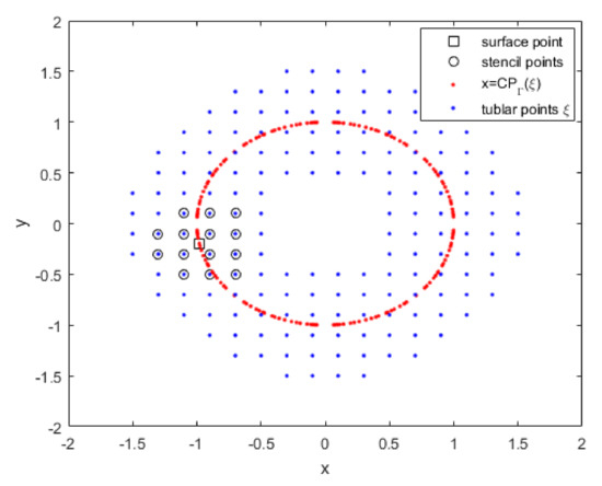
Figure 1. A scheme of the closest points (red dots) to the tubular points in the computational domain (blue dots) on the surface and m = 14 point stencil (circled blue dots) for a surface point (squared red dot).

The combined RBF and polynomial interpolant is assumed to be a linear combination of the radial and polynomial functions; thus, it takes the form

$$\widehat{u}\left(\mathbf{\xi }\right)=\sum _{i=1}^{n_c}{\lambda }_i\varphi (\parallel {\mathbf{\xi }}_j-{\mathbf{\xi }}_i\parallel )+\sum _{i=1}^{n_p}{\gamma }_i{p}_i\left({\mathbf{\xi }}_j\right)$$

(15)

where $\varphi (.)$ is a radial basis function, $p_i(.)$ is the $i-$th monomial in the polynomial basis function in the space coordinates ${\mathbf{x}}^T=[x,y,z]$, and $n_p$ is the number of monomials. To solve for the unknowns, we force the interpolant to match the data at the point locations

$$\widehat{u}\left({\mathbf{\xi }}_j\right)\simeq s\left({\mathbf{\xi }}_j\right)=\sum _{i=1}^{n_c}{\lambda }_i\varphi (\parallel {\mathbf{\xi }}_j-{\mathbf{\xi }}_i\parallel )+\sum _{i=1}^{n_p}{\gamma }_i{p}_i\left({\mathbf{\xi }}_j\right)$$

(16)

where $\varphi (.)$ is a radial basis function, $p_i(.)$ is the $i-$th monomial in the polynomial basis function in the space coordinates ${\mathbf{x}}^T=[x,y,z]$, and $n_p$ is the number of monomials. Moreover, to find an unique result for unknown coefficients, the following $n_c$ constraint orthogonality conditions are imposed

$$\sum _{i=1}^{n_c}{\lambda }_i{p}_k\left({\mathbf{\xi }}_i\right)=0,k=1,\cdots ,n_p,$$

(17)

Equations (15) and (16) are arranged in a linear system of $n_c+n_p$ equations for the $n_c+n_p$ unknowns ${\left\{{\lambda }_i\right\}}_{i=1}^{n_c}\cup {\left\{{\gamma }_i\right\}}_{i=1}^{n_p}$ as follows:

$$\begin{array}{c}\hfill \underset{M}{\underbrace{\left[\begin{array}{cccccc}& & & & & \\ & \mathcal{R}& & & \mathcal{P}& \\ & & & & & \\ & & & & & \\ & & & & & \\ & & & & & \\ & {\mathcal{P}}^T& & & 0& \\ & & & & & \end{array}\right]}}\underset{\Lambda }{\underbrace{\left[\begin{array}{c}{\lambda }_1\\ ⋮\\ {\lambda }_{n_c}\\ \\ {\gamma }_1\\ ⋮\\ {\gamma }_{n_p}\end{array}\right]}}=\underset{C}{\underbrace{\left[\begin{array}{c}\widehat{u}\left({\mathbf{\xi }}_1\right)\\ ⋮\\ \widehat{u}\left({\mathbf{\xi }}_{n_c}\right)\\ \\ 0\\ ⋮\\ 0\end{array}\right]}},\end{array}$$

(18)

where the coefficient matrix M is a non-singular $(n_c+n_p)\times (n_c+n_p)$ matrix [16,38], in which

$$\begin{array}{ccc}& & {\left[\mathcal{R}\right]}_{ij}=\varphi \parallel {\mathbf{\xi }}_j-{\mathbf{\xi }}_i\parallel ,1\le i,j\le n_c,\hfill \\ & & {\left[\mathcal{P}\right]}_{ij}=p_i\left({\mathbf{\xi }}_j\right),1\le i\le n_p,1\le j\le n_c,\hfill \end{array}$$

(19)

and 0 is the $n_p\times n_p$ zero matrix. Therefore, solving the linear system (18) yields the unknown coefficients as follows:

$$\Lambda =M^{-1}C$$

(20)

Evaluating the operator $\mathcal{L}$ of the interpolant at ${\mathbf{x}}_e$ and using relation (20) give

$$\begin{array}{ccc}\hfill \mathcal{L}\widehat{u}\left({\mathbf{x}}_e\right)& =& \sum _{i=1}^{n_c}{\lambda }_i\mathcal{L}\varphi (\parallel {\mathbf{x}}_e-{\mathbf{\xi }}_i\parallel )+\sum _{i=1}^{n_p}{\gamma }_i\mathcal{L}{p}_i\left({\mathbf{x}}_e\right)\hfill \end{array}$$

(21)

$$\begin{array}{ccc}& =& \underset{B^T}{\underbrace{\left[\mathcal{L}\varphi \parallel {\mathbf{x}}_e-{\mathbf{\xi }}_1\parallel \cdots \mathcal{L}\varphi \parallel {\mathbf{x}}_e-{\mathbf{\xi }}_{n_c}\parallel \mathcal{L}{p}_1\left({\mathbf{x}}_e\right)\cdots \mathcal{L}{p}_{n_p}\left({\mathbf{x}}_e\right)\right]}}\Lambda \hfill \end{array}$$

(22)

$$\begin{array}{ccc}\hfill & =& \left(B^T{M}^{-1}\right)C\hfill \end{array}$$

(23)

Once multiplied, $B^T{M}^{-1}$ gives the weights vector ${\tilde{W}}_{e\mathcal{L}}=[{\omega }_1,\cdots {\omega }_{n_c},\omega n_c+1,\cdots {\omega }_{n_c+n_p}]$ for approximating $\mathcal{L}\widehat{u}\left({\mathbf{x}}_c\right)$. Therefore, the solution vector ${\tilde{W}}_{j\mathcal{L}}$ in relation (14) could be determined in the following form:

$${\tilde{W}}_{e\mathcal{L}}=B^T{M}^{-1}={[{\omega }_1,{\omega }_2,\cdots ,{\omega }_{n_c},{\omega }_{n_c+1},\cdots ,{\omega }_{n_c+n_p}]}^T.$$

(24)

Note that in the vector ${\tilde{W}}_{e\mathcal{L}}$, the entries ${\omega }_{n_c+1},\cdots ,{\omega }_{n_c+n_p}$ should be scrapped. Hence, the first $n_c$ components of vector ${\tilde{W}}_{e\mathcal{L}}$ are constructed of the weight vector $W{e}_{\mathcal{L}}={[{\omega }_1,{\omega }_2,\cdots ,{\omega }_{n_c}]}^T$ corresponding to stencil points ${\Xi }_j$.

Therefore, for evaluation point ${\mathbf{x}}_e$ on the surface, the local approximation (14) in the related stencil can be written in novel notation as follows:

$$\mathcal{L}\widehat{u}\left({\mathbf{x}}_e\right)\simeq W_{e\mathcal{L}}^T\widehat{u}\left({\mathbf{\xi }}_j\right).$$

(25)

Then, by computing $W_{j\mathcal{L}}$ for all closest points ${\left\{{\mathbf{x}}_j\right\}}_{j=1}^N$, the global sparse $N\times N$ matrix $W_{\mathcal{L}}={\{W_{1\mathcal{L}}{W}_{2\mathcal{L}}\cdots W_{N\mathcal{L}}\}}^T$ could be assembled such that

$$\mathcal{L}{\widehat{U}}_{\mathbf{x}}=W_{\mathcal{L}}{\widehat{U}}_{\mathbf{\xi }}.$$

(26)

where ${\widehat{U}}_{\mathbf{x}}={[\widehat{u}\left({\mathbf{x}}_1\right)\widehat{u}\left({\mathbf{x}}_2\right)\cdots \widehat{u}\left({\mathbf{x}}_N\right)]}^T$ and ${\widehat{U}}_{\mathbf{\xi }}={[\widehat{u}\left({\mathbf{\xi }}_1\right)\widehat{u}\left({\mathbf{\xi }}_2\right)\cdots \widehat{u}\left({\mathbf{\xi }}_N\right)]}^T.$ For computing the numerical solutions of the problem (12), each differential operator is replaced by the relation (26) in the following form:

$$\begin{array}{c}(1+\tau F)W_I{\widehat{U}}_{\mathbf{\xi }}^{n+1}-\tau \nabla D_{\widehat{u}}^{n+1}{W}_{\nabla }{\widehat{U}}_{\mathbf{\xi }}^{n+1}-\tau D_{\widehat{u}}^{n+1}{W}_{{\nabla }^2}{\widehat{U}}_{\mathbf{\xi }}^{n+1}=-\tau {\mathcal{G}}^{n+1}+\tau F+W_I{\widehat{U}}_{\mathbf{\xi }}^n,\hfill \\ (1+\tau (F+K))W_I{\widehat{V}}_{\mathbf{\xi }}^{n+1}-\tau \nabla D_{\widehat{v}}^{n+1}{W}_{\nabla }{\widehat{V}}_{\mathbf{\xi }}^{n+1}-\tau D_{\widehat{v}}^{n+1}{W}_{{\nabla }^2}{\widehat{V}}_{\mathbf{\xi }}^{n+1}=\tau {\mathcal{G}}^{n+1}+W_I{\widehat{V}}_{\mathbf{\xi }}^n.\hfill \end{array}$$

(27)

Therefore, relation (27) can be rewritten as follows:

$$\begin{array}{c}{A}_u{\widehat{U}}_{\mathbf{\xi }}^{n+1}=-\tau {\mathcal{G}}^{n+1}+\tau F+B_u{\widehat{U}}_{\mathbf{\xi }}^n,\hfill \\ A_v{\widehat{V}}_{\mathbf{\xi }}^{n+1}=\tau {\mathcal{G}}^{n+1}+B_v{\widehat{V}}_{\mathbf{\xi }}^n,\hfill \end{array}$$

(28)

where the $N\times N$ matrices $A_u$, $A_v$, $B_u$, and $B_v$ are defined in the following forms:

$$\begin{array}{c}{A}_u=(1+\tau F)W_I-\tau \nabla D_{\widehat{u}}^{n+1}{W}_{\nabla }-\tau D_{\widehat{u}}^{n+1}{W}_{{\nabla }^2},\hfill \\ A_v=(1+\tau (F+K))W_I-\tau \nabla D_{\widehat{v}}^{n+1}{W}_{\nabla }-\tau D_{\widehat{v}}^{n+1}{W}_{{\nabla }^2},\hfill \\ B_u=W_I,\hfill \\ B_v=W_I.\hfill \end{array}$$

(29)

In numerical implementation to face the non-linear term $\mathcal{G}$, a predictor–corrector Algorithm 1 is used.

Algorithm 1 Predictor–corrector algorithm

Consider initial guesses ${\widehat{U}}_{\mathbf{\xi }}^{n+1,*}\leftarrow {\widehat{U}}_{\mathbf{\xi }}^n$ and ${\widehat{V}}_{\mathbf{\xi }}^{n+1,*}\leftarrow {\widehat{V}}_{\mathbf{\xi }}^n$ $switch=1$ while$switch>0$do    Solve system (28) as follows:     $\begin{array}{c}{A}_u{\widehat{U}}_{\mathbf{\xi }}^{n+1}=-\tau \mathcal{G}({\widehat{U}}_{\mathbf{\xi }}^{n+1,*},{\widehat{V}}_{\mathbf{\xi }}^{n+1,*})+\tau F+B_u{\widehat{U}}_{\mathbf{\xi }}^n,\hfill \end{array}$     $\begin{array}{c}{A}_v{\widehat{V}}_{\mathbf{\xi }}^{n+1}=\tau \mathcal{G}({\widehat{U}}_{\mathbf{\xi }}^{n+1,*},{\widehat{V}}_{\mathbf{\xi }}^{n+1,*})+B_v{\widehat{V}}_{\mathbf{\xi }}^n,\hfill \end{array}$    if $\parallel {\widehat{U}}_{\mathbf{\xi }}^{n+1,*}-{\widehat{U}}_{\mathbf{\xi }}^{n+1}\parallel <{\epsilon }_1$ and $\parallel {\widehat{V}}_{\mathbf{\xi }}^{n+1,*}-{\widehat{V}}_{\mathbf{\xi }}^{n+1}\parallel <{\epsilon }_2$ then     $switch=-1$,    else     ${\widehat{U}}_{\mathbf{\xi }}^{n+1,*}\leftarrow {\widehat{U}}_{\mathbf{\xi }}^{n+1}$ and ${\widehat{V}}_{\mathbf{\xi }}^{n+1,*}\leftarrow {\widehat{V}}_{\mathbf{\xi }}^{n+1}$.    end if end while

Moreover, for implementing the procedure, the thin plate spline (TPS) RBFs

$$\varphi \left(r\right)=r^{2p}ln\left(r\right),p=1,2,\cdots ,$$

(30)

and generalized multiquadric (GMQ) RBFs

$$\varphi \left(r\right)={(1+{\left(cr\right)}^2)}^q,c>0,$$

(31)

are applied. These radial basis functions depend on scatter points on the computational domain, such as ${\mathbf{x}}^T=[x,y,z]$ through the radial variable $r=\sqrt{{(x-x_i)}^2+{(y-y_i)}^2+{(z-z_i)}^2}$, which is the Euclidean distance between the point of interest $\mathbf{x}$ and a computational point ${\mathbf{x}}_i$ in three-dimensional space. The TPS belongs to $C^{2p-1}$ and has strictly conditionally positive definite radial functions of order $p+1$ [16,38]. Moreover, The GMQ belongs to $C^{\infty }$, and for $0<q<1$, it has a strictly, conditionally positive definite order of one [38]. Moreover, for $q=0.5$ we have the standard multiquadric (MQ) RBFs. The accuracy and stability of the methods based on the GMQ radial basis functions depend on the shape parameter c. Furthermore, a set of three-dimensional quadratic monomial basis functions $\{1,x,y,z,x^2,y^2,z^2,xy,xz,yz,xyz\}$ is used to implement the procedure. It is noteworthy that adding polynomials and constructing the augmented RBFs, which guarantee the non-singularity and uniquely solvability of the linear system when using conditionally positive RBFs, could improve the accuracy of the numerical results [39]. Therefore, adding polynomials could improve the stability of the procedure using RBFs. Furthermore, the shape parameters’ sensitivity is reduced by augmenting the polynomials into RBFs, and the range of selection of the shape parameters is extended [40].

To verify the numerical stability of the proposed method, the noise effects on error estimates are investigated. For this purpose, we suppose that the initial solutions $u_0$ and $v_0$ in the numerical process are perturbed to ${\tilde{u}}_0=(1+\delta )u_0$ and ${\tilde{v}}_0=(1+\delta )v_0$, respectively. Therefore, the influence of noise $\delta$ on error estimates is studied for perturbation solutions ${\tilde{u}}_n$ and ${\tilde{v}}_n$ at $T=1$.

4. Numerical Results

In this section, the proposed technique’s performance and accuracy in dealing with the GS system with variable coefficients (2) are verified. The suggested method is implemented to solve four test problems. In the numerical implementation, a tubular-embedding computational domain with a radius of $r_{\Omega }$ and N uniformly distributed nodes surrounding the intended surface is considered. Furthermore, the shape parameters’ sensitivity is reduced by augmenting the polynomials into RBFs, and the range of selection of the shape parameters is extended [40]. Furthermore, The TPS radial basis function (30) with $p=2$ and the MQ radial basis function combined with three-dimensional quadratic monomials basis functions are used to construct shape functions. The root mean square error $\left({ϵ}_r\right)$ and maximum absolute error $\left({ϵ}_{\infty }\right)$ are considered to measure the accuracy of the following method:

$$\begin{array}{ccc}& & {ϵ}_r=\underset{t\in [0,T]}{max}\sqrt{\frac{{\sum }_{i=1}^N{(w_e({\mathbf{x}}_i,t)-w_a({\mathbf{x}}_i,t))}^2}{N}},\hfill \\ & & {ϵ}_{\infty }=\underset{t\in [0,T]}{max}{\parallel w_e(\mathbf{x},t)-w_a(\mathbf{x},t)\parallel }_{\infty },\hfill \end{array}$$

which is applied to make comparisons, where $w_e(\mathbf{x},t)$ and $w_a(\mathbf{x},t)$ demonstrate the exact and approximate solutions, respectively. Furthermore, to verify convergence rates of the presented time discretization scheme, the following rate is calculated:

$${\mathcal{R}}_{ϵ}=\frac{log({ϵ}_{\infty }\left({\tau }_1\right)/{ϵ}_{\infty }\left({\tau }_2\right))}{log({\tau }_1/{\tau }_2)}.$$

Example 1.

As the first example, we consider the following problem on a sphere with radius of one and a center of zero:

$$\begin{array}{c}\frac{\partial u}{\partial t}={\nabla }_{\Gamma }.\left[{10}^{-3}uv{\nabla }_{\Gamma }u\right]-u{v}^2+20(1-u),\hfill \\ \frac{\partial v}{\partial t}={\nabla }_{\Gamma }.\left[{10}^{-3}uv{\nabla }_{\Gamma }v\right]+u{v}^2-20v.\hfill \end{array}$$

The exact solutions of Equation (1) are

$$\begin{array}{c}u(x,y,t)=\frac{1}{2}sin\left(t\right)cos\left(\pi x\right)cos\left(\pi y\right)cos\left(\pi z\right),\hfill \\ v(x,y,t)=\frac{1}{4}sin\left(t\right)cos\left(\pi x\right)cos\left(\pi y\right)cos\left(\pi z\right).\hfill \end{array}$$

The proposed numerical technique is applied to solve the problem. The resulting error estimates and CPU times for various values of N by letting $\tau =0.5{\left(dx\right)}^2$ for two different RBFs are reported in Table 1. As observed, by increasing the number of computational points, the suggested numerical method’s accuracy is improved. Table 2 demonstrates the estimated errors and computational temporal convergence rate ${\mathcal{R}}_{ϵ}$ in terms of time step sizes $\tau$. The results are obtained by introducing stencil size $n_s=33$ and $N=2670$ data points in the TPS and MQ cases. The shape parameter for the MQ radial basis function is $c=0.35$. The given results show the first-order convergence of the proposed temporal discretization scheme. Furthermore, the suggested method’s stability is reported in Table 3. This table shows the impression of the noise $\left(\delta \right)$ on absolute computational errors and indicates that the proposed method has a reasonable and stable behaviour against the enforcing noise. Moreover, the graphs of exact and computed solutions related to u and v by taking $N=4416$, $n_s=33$, and $\tau =0.5{\left(dx\right)}^2$ for TPS radial basis functions are shown in Figure 2. Furthermore, the coefficient matrix’s sparsity pattern for two types of RBFs is plotted in Figure 3.

Table 1. Error estimates and CPU times of Example 1 by letting $\tau =0.5{\left(dx\right)}^2$ for different values of $dx$, and stencil size $n_s$.

				TPS				MQ
$\mathit{dx}$	$\mathit{N}$	${\mathit{n}}_{\mathit{s}}$	Variables	${\mathbf{ϵ}}_{\infty }$	${\mathbf{ϵ}}_{\mathit{r}}$	Time		$\mathit{c}$	${\mathbf{ϵ}}_{\infty }$	${\mathbf{ϵ}}_{\mathit{r}}$	Time
$\frac{1}{2}$	408	23	u	$4.1486\times {10}^{-4}$	$4.3919\times {10}^{-4}$	$0.9821$		0.10	$4.4010\times {10}^{-4}$	$4.3779\times {10}^{-4}$	$1.0046$
			v	$2.2143\times {10}^{-4}$	$2.2009\times {10}^{-4}$				$2.2055\times {10}^{-4}$	$2.1939\times {10}^{-4}$
$\frac{1}{4}$	1320	27	u	$2.6649\times {10}^{-4}$	$1.1915\times {10}^{-4}$	$1.8851$		0.20	$2.5918\times {10}^{-4}$	$1.1650\times {10}^{-4}$	$2.0103$
			v	$1.3479\times {10}^{-4}$	$6.0050\times {10}^{-5}$				$1.3110\times {10}^{-4}$	$5.8701\times {10}^{-5}$
$\frac{1}{6}$	2640	30	u	$1.4240\times {10}^{-4}$	$5.6536\times {10}^{-5}$	$3.3515$		0.30	$1.3717\times {10}^{-4}$	$5.5761\times {10}^{-5}$	$3.8863$
			v	$7.2269\times {10}^{-5}$	$2.8490\times {10}^{-5}$				$6.9622\times {10}^{-5}$	$2.8094\times {10}^{-5}$
$\frac{1}{8}$	4416	33	u	$9.0510\times {10}^{-5}$	$3.3602\times {10}^{-5}$	$6.8865$		0.40	$8.7769\times {10}^{-5}$	$3.3398\times {10}^{-5}$	$7.3159$
			v	$4.4598\times {10}^{-5}$	$1.6814\times {10}^{-5}$				$4.0514\times {10}^{-5}$	$1.0144\times {10}^{-5}$
$\frac{1}{10}$	6912	36	u	$6.4931\times {10}^{-5}$	$2.3586\times {10}^{-5}$	$13.1929$		0.50	$6.3311\times {10}^{-5}$	$2.3627\times {10}^{-5}$	$14.3260$
			v	$3.3009\times {10}^{-5}$	$1.1874\times {10}^{-5}$				$3.2186\times {10}^{-5}$	$1.1893\times {10}^{-5}$
$\frac{1}{12}$	9936	39	u	$4.9980\times {10}^{-5}$	$1.8055\times {10}^{-5}$	$24.9908$		0.60	$4.8150\times {10}^{-5}$	$1.8046\times {10}^{-5}$	$27.6299$
			v	$2.5415\times {10}^{-5}$	$9.0903\times {10}^{-6}$				$2.4485\times {10}^{-5}$	$9.0848\times {10}^{-6}$

Table 2. Error estimates and CPU times of Example 1 by letting $dx=\frac{1}{7}$, stencil size $n_s=33$, and $c=0.35$ for different values of $\tau$.

		TPS				MQ
$\mathbf{\tau }$	Variables	${\mathbf{ϵ}}_{\infty }$	${\mathbf{ϵ}}_{\mathit{r}}$	${\mathcal{R}}_{\mathbf{ϵ}}$		${\mathbf{ϵ}}_{\infty }$	${\mathbf{ϵ}}_{\mathit{r}}$	${\mathcal{R}}_{\mathbf{ϵ}}$
$d{x}^2$	u	$1.0129\times {10}^{-4}$	$3.9335\times {10}^{-5}$	−		$1.0131\times {10}^{-4}$	$3.9279\times {10}^{-5}$	−
	v	$5.0860\times {10}^{-5}$	$1.9706\times {10}^{-5}$	−		$5.0869\times {10}^{-5}$	$1.9678\times {10}^{-5}$	−
$\frac{1}{2}d{x}^2$	u	$5.3413\times {10}^{-5}$	$2.0678\times {10}^{-5}$	$0.9232$		$5.3423\times {10}^{-5}$	$2.0620\times {10}^{-5}$	$0.9232$
	v	$2.6821\times {10}^{-5}$	$1.0359\times {10}^{-5}$	$0.9231$		$2.6826\times {10}^{-5}$	$1.0330\times {10}^{-5}$	$0.9231$
$\frac{1}{4}d{x}^2$	u	$2.7287\times {10}^{-5}$	$1.0797\times {10}^{-5}$	$0.9689$		$2.6501\times {10}^{-5}$	$1.0746\times {10}^{-5}$	$1.0114$
	v	$1.3699\times {10}^{-5}$	$5.4088\times {10}^{-6}$	$0.9692$		$1.3303\times {10}^{-5}$	$5.3833\times {10}^{-5}$	$1.0118$
$\frac{1}{8}d{x}^2$	u	$1.0929\times {10}^{-5}$	$5.9440\times {10}^{-6}$	$1.3200$		$1.0829\times {10}^{-5}$	$5.8848\times {10}^{-6}$	$1.2911$
	v	$5.4796\times {10}^{-6}$	$2.9766\times {10}^{-6}$	$1.5814$		$5.4293\times {10}^{-6}$	$2.9469\times {10}^{-6}$	$1.2929$

Table 3. The effect of noise on error estimates of Example 1 for $N=1848$, $\tau =0.5{\left(dx\right)}^2$, and $n_c=27$.

		TPS		MQ
$\mathbf{\delta }$	Variables	${\mathbf{ϵ}}_{\infty }$		${\mathbf{ϵ}}_{\infty }$
0	u	$1.8968\times {10}^{-4}$		$1.8538\times {10}^{-4}$
	v	$9.6149\times {10}^{-5}$		$9.3972\times {10}^{-5}$
$0.001$	u	$2.0232\times {10}^{-4}$		$1.9802\times {10}^{-4}$
	v	$1.0256\times {10}^{-4}$		$1.0038\times {10}^{-4}$
$0.01$	u	$3.1611\times {10}^{-4}$		$3.1177\times {10}^{-4}$
	v	$1.6033\times {10}^{-4}$		$1.5813\times {10}^{-4}$
$0.1$	u	$1.4527\times {10}^{-3}$		$1.4448\times {10}^{-3}$
	v	$7.3918\times {10}^{-4}$		$7.3679\times {10}^{-4}$

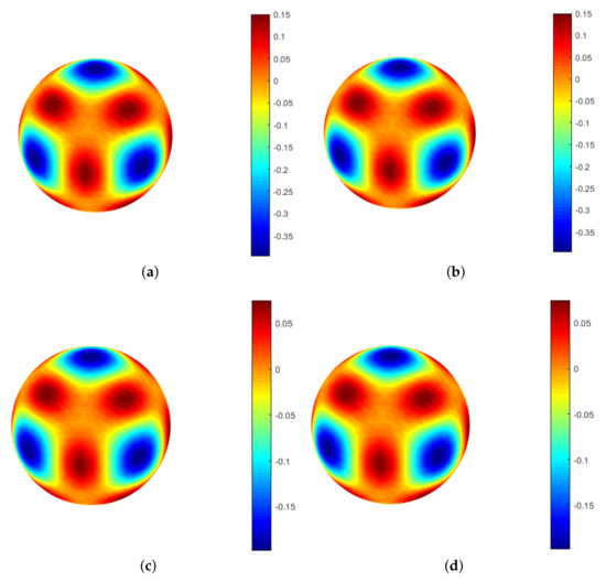
Figure 2. Plot of the exact solution (a) and plot of the approximate solution (b) related to u, and plot of the exact solution (c) and plot of the approximate solution (d) related to v with TPS for Example 1 by taking $dx=\frac{1}{8}$ and $\tau =0.5d{x}^2$.

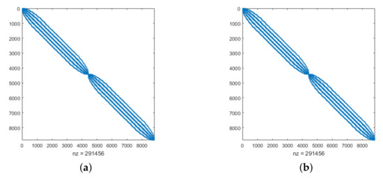
Figure 3. Sparsity pattern for Example 1 with (a) TPS and (b) MQ by taking $dx=\frac{1}{8}$, $\tau =d{x}^2$, and $n_c=33$.

Example 2.

As the second example, we consider the following problem:

$$\begin{array}{c}\frac{\partial u}{\partial t}={\nabla }_{\Gamma }.\left[{10}^{-4}{u}^2{\nabla }_{\Gamma }u\right]-u{v}^2+10(1-u),\hfill \\ \frac{\partial v}{\partial t}={\nabla }_{\Gamma }.\left[{10}^{-4}{v}^2{\nabla }_{\Gamma }v\right]+u{v}^2-(10+0.01)v.\hfill \end{array}$$

on the irregular bumpy sphere

$$\Gamma =(x,y,z):x=rsin\theta cos\phi ,y=rsin\theta sin\phi ,z=rcos\phi ,0\le \theta \le 2\pi ,0\le \phi \le \pi ,$$

where

$$r=1+\frac{1}{7}sin\left(6\theta \right)sin\left(7\phi \right).$$

The exact solutions of Equation (2) are

$$\begin{array}{c}u(x,y,t)=\frac{1}{2}exp(-t)cos\left(\pi x\right)cos\left(\pi y\right)cos\left(\pi z\right),\hfill \\ v(x,y,t)=\frac{1}{2}exp(-t)sin\left(\pi x\right)sin\left(\pi y\right)sin\left(\pi z\right).\hfill \end{array}$$

The presented computational technique is used to solve this example. Several reports are given to verify the accuracy and efficiency of the suggested procedure. Table 4 reports the absolute and RMS errors and CPU times of the various values of N by taking $\tau =0.5{\left(dx\right)}^2$ for the two kinds of RBFs tat are presented. This table shows the accuracy and convergence of the method by increasing the number of computational points. In Table 5, the absolute and RMS errors and computational temporal convergence rate ${\mathcal{R}}_{ϵ}$ in terms of time step sizes $\tau$ are demonstrated. The results are given by taking stencil size $n_s=35$ and $N=4509$ data points for the two kinds of RBFs. The obtained numerical results illustrate the first-order convergence of the proposed temporal discretization scheme. Moreover, the proposed numerical method’s stability affected by the noise $\left(\delta \right)$ on absolute computational errors is reported in Table 6. In addition, the graphs of exact and computed solutions related to u and v are shown in Figure 4. These results are achieved by letting $N=4509$, $n_s=35$, and $\tau =0.5{\left(dx\right)}^2$ for TPS radial basis function. The sparsity pattern of the coefficient matrix for two types of RBFs is plotted in Figure 5.

Table 4. Error estimates and CPU times of Example 2 by letting $\tau =0.5{\left(dx\right)}^2$ for different values of $dx$ and stencil size $n_s$.

				TPS				MQ
$\mathit{dx}$	$\mathit{N}$	${\mathit{n}}_{\mathit{s}}$	Variables	${\mathbf{ϵ}}_{\infty }$	${\mathbf{ϵ}}_{\mathit{r}}$	Time		$\mathit{c}$	${\mathbf{ϵ}}_{\infty }$	${\mathbf{ϵ}}_{\mathit{r}}$	Time
$\frac{1}{2}$	401	23	u	$4.7199\times {10}^{-4}$	$4.7145\times {10}^{-4}$	$0.9295$		0.10	$4.7202\times {10}^{-4}$	$4.7161\times {10}^{-4}$	$1.2348$
			v	$4.7362\times {10}^{-4}$	$4.7200\times {10}^{-4}$				$4.7418\times {10}^{-4}$	$4.7246\times {10}^{-4}$
$\frac{1}{4}$	1257	29	u	$2.5693\times {10}^{-4}$	$1.1483\times {10}^{-4}$	$1.7973$		0.20	$2.5740\times {10}^{-4}$	$1.1510\times {10}^{-4}$	$2.1156$
			v	$2.5571\times {10}^{-4}$	$1.1471\times {10}^{-4}$				$2.5729\times {10}^{-4}$	$1.1530\times {10}^{-4}$
$\frac{1}{6}$	2608	32	u	$1.2988\times {10}^{-4}$	$5.1986\times {10}^{-5}$	$3.6231$		0.30	$1.3095\times {10}^{-4}$	$5.2074\times {10}^{-5}$	$4.2815$
			v	$1.2887\times {10}^{-4}$	$4.7212\times {10}^{-5}$				$1.3001\times {10}^{-4}$	$4.7452\times {10}^{-5}$
$\frac{1}{8}$	4509	35	u	$7.6720\times {10}^{-5}$	$2.9180\times {10}^{-5}$	$7.1556$		0.40	$7.7605\times {10}^{-5}$	$2.9222\times {10}^{-5}$	$8.2007$
			v	$7.6123\times {10}^{-5}$	$2.6934\times {10}^{-5}$				$7.6694\times {10}^{-5}$	$2.7073\times {10}^{-5}$
$\frac{1}{10}$	7049	37	u	$5.0690\times {10}^{-5}$	$1.8478\times {10}^{-5}$	$14.0363$		0.50	$5.1322\times {10}^{-5}$	$1.8497\times {10}^{-5}$	$16.6223$
			v	$4.9984\times {10}^{-5}$	$1.7654\times {10}^{-5}$				$5.0342\times {10}^{-5}$	$1.7744\times {10}^{-5}$
$\frac{1}{12}$	10114	40	u	$3.6096\times {10}^{-5}$	$1.2770\times {10}^{-5}$	$28.4784$		0.60	$3.6423\times {10}^{-5}$	$1.2786\times {10}^{-5}$	$29.3094$
			v	$3.5423\times {10}^{-5}$	$1.2567\times {10}^{-5}$				$3.5701\times {10}^{-5}$	$1.2634\times {10}^{-5}$

Table 5. Error estimates and CPU times of Example 2 by letting $dx=\frac{1}{8}$, stencil size $n_s=35$, and $c=0.4$ for different values of $\tau$.

		TPS				MQ
$\mathbf{\tau }$	Variables	${\mathbf{ϵ}}_{\infty }$	${\mathbf{ϵ}}_{\mathit{r}}$	${\mathcal{R}}_{\mathbf{ϵ}}$		${\mathbf{ϵ}}_{\infty }$	${\mathbf{ϵ}}_{\mathit{r}}$	${\mathcal{R}}_{\mathbf{ϵ}}$
$dx$	u	$1.9579\times {10}^{-3}$	$7.5409\times {10}^{-4}$	−		$1.9615\times {10}^{-3}$	$7.5426\times {10}^{-4}$	−
	v	$1.9542\times {10}^{-3}$	$6.9668\times {10}^{-4}$	−		$1.9564\times {10}^{-3}$	$6.9704\times {10}^{-4}$	−
$\frac{1}{2}dx$	u	$9.8855\times {10}^{-4}$	$3.7975\times {10}^{-4}$	$0.9859$		$9.9231\times {10}^{-4}$	$3.7993\times {10}^{-4}$	$0.9830$
	v	$9.8555\times {10}^{-4}$	$3.5080\times {10}^{-4}$	$0.9875$		$9.8781\times {10}^{-4}$	$3.5118\times {10}^{-4}$	$0.9858$
$\frac{1}{4}dx$	u	$4.9720\times {10}^{-4}$	$1.9003\times {10}^{-4}$	$0.9914$		$5.0101\times {10}^{-4}$	$1.9021\times {10}^{-4}$	$0.9859$
	v	$4.9457\times {10}^{-4}$	$1.7551\times {10}^{-4}$	$0.9947$		$4.9686\times {10}^{-4}$	$1.7589\times {10}^{-4}$	$0.9913$
$\frac{1}{8}dx$	u	$2.5103\times {10}^{-4}$	$9.4987\times {10}^{-5}$	$0.9859$		$2.5485\times {10}^{-4}$	$9.5169\times {10}^{-5}$	$0.9751$
	v	$2.4858\times {10}^{-4}$	$8.7699\times {10}^{-5}$	$0.9924$		$2.5088\times {10}^{-4}$	$8.8082\times {10}^{-5}$	$0.9858$

Table 6. The effect of noise on error estimates of Example 2 for $N=1862$, $\tau =0.5{\left(dx\right)}^2$, and $n_c=27$.

		TPS		MQ
$\mathbf{\delta }$	Variables	${\mathbf{ϵ}}_{\infty }$		${\mathbf{ϵ}}_{\infty }$
0	u	$1.7948\times {10}^{-4}$		$1.7941\times {10}^{-4}$
	v	$2.0621\times {10}^{-4}$		$2.0791\times {10}^{-4}$
$0.001$	u	$1.9725\times {10}^{-4}$		$1.9718\times {10}^{-4}$
	v	$2.2684\times {10}^{-4}$		$2.2854\times {10}^{-4}$
$0.01$	u	$3.5719\times {10}^{-4}$		$3.5712\times {10}^{-4}$
	v	$4.1253\times {10}^{-4}$		$4.1425\times {10}^{-4}$
$0.1$	u	$1.9556\times {10}^{-3}$		$1.9565\times {10}^{-3}$
	v	$2.2694\times {10}^{-3}$		$2.2713\times {10}^{-3}$

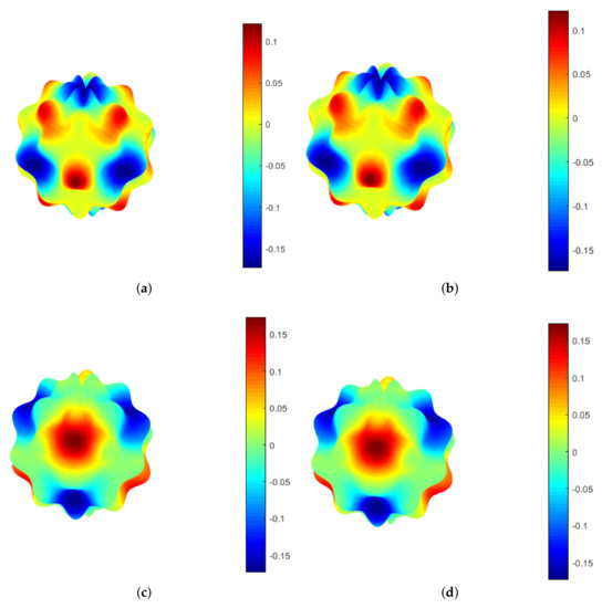
Figure 4. Plot of the exact solution (a) and plot of the approximate solution (b) related to u, and plot of the exact solution (c) and plot of the approximate solution (d) related to v with TPS for Example 2 by taking $dx=\frac{1}{8}$ and $\tau =0.5d{x}^2$.

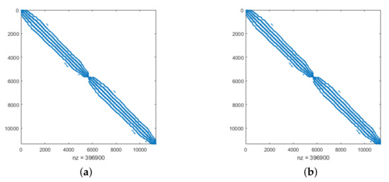
Figure 5. Sparsity pattern for Example 2 with (a) TPS and (b) MQ by taking $dx=\frac{1}{9}$, $\tau =d{x}^2$, and $n_c=35$.

Example 3.

As the third example, we consider the following problem on a ellipsoidal surface:

$$\begin{array}{c}\frac{\partial u}{\partial t}={\nabla }_{\Gamma }.\left[{10}^{-4}u{\nabla }_{\Gamma }u\right]-u{v}^2+5(1-u),\hfill \\ \frac{\partial v}{\partial t}={\nabla }_{\Gamma }.\left[{10}^{-4}v{\nabla }_{\Gamma }v\right]+u{v}^2-(5+0.01)v.\hfill \end{array}$$

on the ellipsoidal surface

$$\Gamma =(x,y,z):x=rcos\theta cos\phi ,y=rcos\theta sin\phi ,z=rsin\phi ,-\frac{\pi }{2}\le \theta \le \frac{\pi }{2},0\le \phi \le 2\pi ,$$

where

$$r=\frac{0.{75}^2\times 1.25}{\sqrt{1.{25}^2(0.{75}^2{cos}^2\phi +0.{75}^2{sin}^2\phi ){cos}^2\theta +0.{75}^4{sin}^2\theta }}.$$

The exact solutions of Equation (3) are

$$\begin{array}{c}u(x,y,t)=cos\left(\frac{1}{4}(x+y+z-t)\right),\hfill \\ v(x,y,t)=sin\left(\frac{1}{4}(x+y+z-t)\right).\hfill \end{array}$$

The suggested numerical method is applied to solve this example. The computational results show the accuracy and efficiency of the proposed technique. The accuracy and convergence of the numerical technique in terms of the number of computational points N are demonstrated in Table 7. In this table, the error estimates and CPU time are obtained by letting $\tau =0.5{\left(dx\right)}^2$ for both TPS and MQ radial basis functions. The computational error estimates and convergence rate in terms of time step size are reported in Table 8. The achieved numerical results are computed by letting $N=2670$ and $n_s=33$. The results show that the computational convergence rate ${\mathcal{R}}_{ϵ}$ follows the analytical convergence rate $\mathcal{O}\left(\tau \right)$. Furthermore, the computational method’s stability is investigated by considering the effect of noise $\left(\delta \right)$ on absolute computational errors, as shown in Table 9. The graphs of exact and computed solutions related to u and v are demonstrates in Figure 6. All figures are achieved by letting $N=3316$, $n_s=33$, and $\tau =0.5{\left(dx\right)}^2$ for the TPS radial basis function. Furthermore, the sparsity patterns of the coefficient matrix related to two kinds of RBFs are plotted in Figure 7.

Table 7. Error estimates and CPU times of Example 3 by letting $\tau =0.5{\left(dx\right)}^2$ for different values of $dx$, and stencil size $n_s$.

				TPS				MQ
$\mathit{dx}$	$\mathit{N}$	${\mathit{n}}_{\mathit{s}}$	Variables	${\mathbf{ϵ}}_{\infty }$	${\mathbf{ϵ}}_{\mathit{r}}$	Time		$\mathit{c}$	${\mathbf{ϵ}}_{\infty }$	${\mathbf{ϵ}}_{\mathit{r}}$	Time
$\frac{1}{2}$	400	23	u	$8.8895\times {10}^{-4}$	$7.6597\times {10}^{-4}$	$0.8523$		0.10	$8.8902\times {10}^{-4}$	$7.6596\times {10}^{-4}$	$0.9776$
			v	$7.0625\times {10}^{-4}$	$3.8833\times {10}^{-4}$				$7.0614\times {10}^{-4}$	$3.8834\times {10}^{-4}$
$\frac{1}{4}$	1084	27	u	$1.9633\times {10}^{-4}$	$1.8441\times {10}^{-4}$	$1.7290$		0.20	$1.9630\times {10}^{-4}$	$1.8441\times {10}^{-4}$	$1.7944$
			v	$1.2277\times {10}^{-4}$	$7.0582\times {10}^{-5}$				$1.2275\times {10}^{-4}$	$7.0585\times {10}^{-5}$
$\frac{1}{6}$	2040	30	u	$8.8826\times {10}^{-5}$	$8.3012\times {10}^{-5}$	$2.9296$		0.30	$8.8817\times {10}^{-5}$	$8.3013\times {10}^{-5}$	$3.2686$
			v	$5.0638\times {10}^{-5}$	$2.6842\times {10}^{-5}$				$5.0679\times {10}^{-5}$	$2.6842\times {10}^{-5}$
$\frac{1}{8}$	3316	33	u	$5.1215\times {10}^{-5}$	$4.7909\times {10}^{-5}$	$5.0001$		0.40	$5.1214\times {10}^{-5}$	$4.7907\times {10}^{-5}$	$5.7858$
			v	$2.7470\times {10}^{-5}$	$1.4511\times {10}^{-5}$				$2.7469\times {10}^{-5}$	$1.4508\times {10}^{-5}$
$\frac{1}{10}$	5026	36	u	$3.3824\times {10}^{-5}$	$3.1699\times {10}^{-5}$	$8.5943$		0.50	$3.3821\times {10}^{-5}$	$3.1698\times {10}^{-5}$	$9.6472$
			v	$1.7267\times {10}^{-5}$	$9.4886\times {10}^{-6}$				$1.7291\times {10}^{-5}$	$9.4871\times {10}^{-6}$
$\frac{1}{12}$	7104	39	u	$2.4384\times {10}^{-5}$	$2.2899\times {10}^{-5}$	$14.7785$		0.60	$2.4381\times {10}^{-5}$	$2.2898\times {10}^{-5}$	$16.3848$
			v	$1.2347\times {10}^{-5}$	$6.9526\times {10}^{-6}$				$1.2364\times {10}^{-5}$	$6.9507\times {10}^{-6}$
$\frac{1}{14}$	9500	42	u	$1.8708\times {10}^{-5}$	$1.7598\times {10}^{-5}$	$25.3011$		0.70	$1.8704\times {10}^{-5}$	$1.7597\times {10}^{-5}$	$28.1007$
			v	$9.5094\times {10}^{-6}$	$5.4846\times {10}^{-6}$				$9.5156\times {10}^{-6}$	$5.4822\times {10}^{-6}$

Table 8. Error estimates and CPU times of Example 3 by letting $dx=\frac{1}{7}$, stencil size $n_s=33$, and $c=0.35$ for different values of $\tau$.

		TPS				MQ
$\mathbf{\tau }$	Variables	${\mathbf{ϵ}}_{\infty }$	${\mathbf{ϵ}}_{\mathit{r}}$	${\mathcal{R}}_{\mathbf{ϵ}}$		${\mathbf{ϵ}}_{\infty }$	${\mathbf{ϵ}}_{\mathit{r}}$	${\mathcal{R}}_{\mathbf{ϵ}}$
$dx$	u	$8.8455\times {10}^{-4}$	$7.7656\times {10}^{-4}$	−		$8.8459\times {10}^{-4}$	$7.7657\times {10}^{-4}$	−
	v	$6.5736\times {10}^{-4}$	$2.6026\times {10}^{-4}$	−		$6.5742\times {10}^{-4}$	$2.6026\times {10}^{-4}$	−
$\frac{1}{2}dx$	u	$4.2416\times {10}^{-4}$	$4.0695\times {10}^{-4}$	$1.0603$		$4.2422\times {10}^{-4}$	$4.0695\times {10}^{-4}$	$1.0601$
	v	$2.8983\times {10}^{-4}$	$1.2418\times {10}^{-4}$	$1.1814$		$2.8990\times {10}^{-4}$	$1.2418\times {10}^{-4}$	$1.1812$
$\frac{1}{4}dx$	u	$2.0447\times {10}^{-4}$	$2.0144\times {10}^{-4}$	$1.0527$		$2.0449\times {10}^{-4}$	$2.0144\times {10}^{-4}$	$1.0527$
	v	$1.2432\times {10}^{-4}$	$5.6703\times {10}^{-5}$	$1.2211$		$1.2439\times {10}^{-4}$	$5.6702\times {10}^{-5}$	$1.2206$
$\frac{1}{8}dx$	u	$1.0449\times {10}^{-4}$	$1.0091\times {10}^{-4}$	$0.9685$		$1.0449\times {10}^{-4}$	$1.0091\times {10}^{-4}$	$0.9686$
	v	$5.6503\times {10}^{-5}$	$2.7500\times {10}^{-5}$	$1.1376$		$5.6573\times {10}^{-5}$	$2.7498\times {10}^{-5}$	$1.1366$

Table 9. The effect of noise on error estimates of Example 3 for $N=1496$, $\tau =0.5{\left(dx\right)}^2$, and $n_c=27$.

		TPS		MQ
$\mathbf{\delta }$	Variables	${\mathbf{ϵ}}_{\infty }$		${\mathbf{ϵ}}_{\infty }$
0	u	$1.2665\times {10}^{-4}$		$1.2664\times {10}^{-4}$
	v	$7.6139\times {10}^{-5}$		$7.6115\times {10}^{-5}$
$0.001$	u	$1.3683\times {10}^{-4}$		$1.3686\times {10}^{-4}$
	v	$1.0696\times {10}^{-4}$		$1.0694\times {10}^{-4}$
$0.01$	u	$3.7383\times {10}^{-4}$		$3.7384\times {10}^{-4}$
	v	$4.8819\times {10}^{-4}$		$4.8819\times {10}^{-4}$
$0.1$	u	$3.8131\times {10}^{-3}$		$3.8131\times {10}^{-3}$
	v	$5.2149\times {10}^{-3}$		$5.2150\times {10}^{-3}$

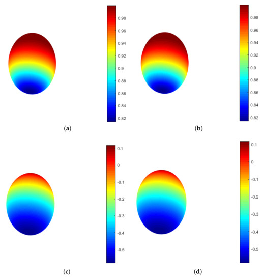
Figure 6. Plot of the exact solution (a) and plot of the approximate solution (b) related to u, and plot of the exact solution (c) and plot of the approximate solution (d) related to v with TPS for Example 2 by taking $dx=\frac{1}{8}$ and $\tau =0.5d{x}^2$.

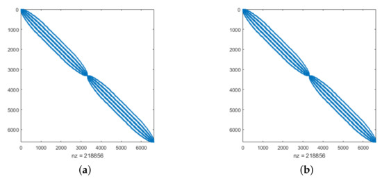
Figure 7. Sparsity pattern for Example 3 with (a) TPS and (b) MQ by taking $dx=\frac{1}{8}$, $\tau =d{x}^2$, and $n_c=33$.

Example 4.

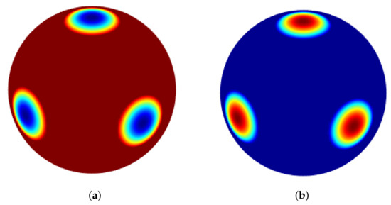
In this example, we examine several practical problems to show that the GS model’s pattern reconstruction property is preserved with variable diffusion coefficients. Considering that in real-world problems, only some conditions such as initial conditions can be determined, the proposed method’s effect and performance in solving the GS model were investigated according to the initial conditions. In these cases, only the initial condition is given on the desired surface. The results show the efficiency of the suggested numerical method in detecting spot and stripe patterns based on the initial condition on the surfaces.

In the first case, we consider a spherical surface with the following initial condition:

$$(u_0,v_0)=\left\{\begin{array}{c}(1,0),x^2\le 1,y^2\le 1,z^2\le 1,\hfill \\ (0,1),o.w.\hfill \end{array}\right.$$

Furthermore, the coefficients are $D_u(x,y,z,t)={10}^{-4}t(x+y+z){.}^2$ and $D_v(x,y,z,t)=5\times {10}^{-5}t{(x+y+z)}^2$. The parameters are $F=20$ and $K={10}^{-3}$. Figure 8 shows the numerical solutions v and u on the spherical surface.

Figure 8. The plot of approximate solution of u (a) and the plot of approximate solution of v (b) with TPS for Example 4 by taking $dx=\frac{1}{8}$, and $\tau =0.5d{x}^2$.

In the second case, we consider a bumpy spherical surface with the following initial condition:

$$(u_0,v_0)=\left\{\begin{array}{c}(1,0),x^2\le 1,y^2\le 1,\hfill \\ (0,1),o.w.\hfill \end{array}\right.$$

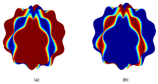
In addition, the coefficients are $D_u(x,y,z,t)={10}^{-4}cos\left(\pi x\right)cos\left(\pi y\right)cos\left(\pi z\right)sin\left(t\right)$ and $D_v(x,y,z,t)=D_u(x,y,z,t)$, and the constant parameters are $F=5$ and $K={10}^{-3}$. Figure 9 shows the numerical solutions v and u on the irregular bumpy sphere surface.

Figure 9. The plot of approximate solution of u (a) and the plot of approximate solution of v (b) with TPS for Example 4 by taking $dx=\frac{1}{8}$, and $\tau =0.5d{x}^2$.

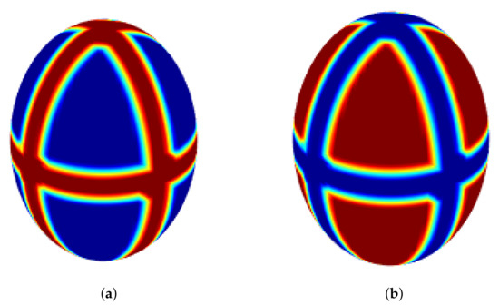
In the third case, we consider an ellipsoidal surface with the following initial condition:

$$u_0=\left\{\begin{array}{c}\frac{1}{4}{cos}^2\left(4\pi x\right){cos}^2\left(4\pi y\right){cos}^2\left(4\pi z\right),0.15\le x^2,y^2\le 1,0.15\le z^2\le 1.25,\hfill \\ 1,o.w.\hfill \end{array}\right.$$

where $v_0=1-u_0$. Additionally, the coefficients are $D_u(x,y,z,t)={10}^{-4}sin\left(\pi x\right)sin\left(\pi y\right)sin\left(\pi z\right)exp\left(t\right)$ and $D_v(x,y,z,t)=D_u(x,y,z,t)$, and the parameters are $F=20$ and $K={10}^{-3}$. Figure 10 shows the approximate solutions v and u on the surface.

Figure 10. The plot of approximate solution of u (a) and the plot of approximate solution of v (b) with TPS for Example 4 by taking $dx=\frac{1}{8}$, and $\tau =0.5d{x}^2$.

As can be seen, in Figure 8, Figure 9 and Figure 10, each pair of shapes corresponds to the variables u and v. Therefore, the inverse colours in these figures are due to different initial conditions for the two variables u and v. That is, each shape represents the pattern recognition corresponding to each variable by different initial conditions.

5. Conclusions

In this work, an advanced and powerful computational technique is used to numerically investigate the three-dimensional Gray–Scott system with variable diffusion coefficients on surfaces. Firstly, the appearing time derivatives are discretized by employing an implicit difference stepping approach. The time-independent discretization problem is solved using a meshfree method based on the combination of RBF-FD and CPM. A meshless local RBF-FD method is used to discretize the governing time-independent problem in the spatial direction. In our implementation, two radial basis functions, thin plate splines and multiquadrics radial basis functions, are used. The presented method is applied to four numerical examples. The presented results, through the tables and figures, show the performance and accuracy of the proposed numerical technique.

References

- Jackson, J.D. Classical Electrodynamics; John Wiley & Sons: New York, NY, USA, 2007. [Google Scholar]
- Carslaw, H.S.; Jaeger, J.C. Conduction of Heat in Solids; Oxford Science Publications: Oxford, UK, 2000. [Google Scholar]
- Crank, J. The Mathematics of Diffusion; Oxford Science Publications: Oxford, UK, 2004. [Google Scholar]
- Bruggeman, G.A. Analytical Solutions of Geohydrological Problems; Elsevier: Amsterdam, The Netherlands, 1999. [Google Scholar]
- Fallico, C.; De Bartolo, S.; Veltri, M.; Severino, G. On the dependence of the saturated hydraulic conductivity upon the effective porosity through a power law model at different scales. Hydrol. Process. 2016, 30, 2366–2372. [Google Scholar] [CrossRef]
- Severino, G. Macrodispersion by Point-Like Source Flows in Randomly Heterogeneous Porous Media. Transp. Porous Media 2011, 89, 121–134. [Google Scholar] [CrossRef]
- Severino, G.; Santini, A.; Monetti, V.M. Modelling Water Flow and Solute Transport in Heterogeneous Unsaturated Porous Media. In Advances in Modeling Agricultural Systems; Springer: New York, NY, USA, 2009; pp. 361–383. [Google Scholar] [CrossRef]
- Severino, G.; Santini, A. On the effective hydraulic conductivity in mean vertical unsaturated steady flows. Adv. Water Resour. 2005, 28, 964–974. [Google Scholar] [CrossRef]
- Turing, A.M. The chemical basis of morphogenesis. Phil. Trans. 1952, 237, 37–72. [Google Scholar]
- Campagna, R.; Cuomo, S.; Giannino, F.; Severino, G.; Toraldo, G. A Semi-Automatic Numerical Algorithm for Turing Patterns Formation in a Reaction-Diffusion Model. IEEE Access 2018, 6, 4720–4724. [Google Scholar] [CrossRef]
- Munafo, R. Reaction-Diffusion by the Gray-Scott Model: Pearson’s pArameterization. Available online: http://mrob.com/pub/comp/xmorphia/index.html (accessed on 26 March 2020).
- Pearson, J.E. Complex patterns in a simple system. Science 1993, 261, 189–192. [Google Scholar] [CrossRef] [PubMed]
- Kansa, E.J. Multiquadrics—A scattered data approximation scheme with applications to computational fluid-dynamics—II solutions to parabolic, hyperbolic and elliptic partial differential equations. Comput. Math. Appl. 1990, 19, 147–161. [Google Scholar] [CrossRef]
- Fasshauer, G.E. Solving differential equations with radial basis functions: Multilevel methods and smoothing. Adv. Comput. Math. 1999, 11, 139–159. [Google Scholar] [CrossRef]
- Larsson, E.; Fornberg, B. A numerical study of some radial basis function based solution methods for elliptic PDEs. Comput. Math. Appl. 2003, 46, 891–902. [Google Scholar] [CrossRef]
- Wendl. Scattered Data Approximation (Cambridge Monographs on Applied and Computational Mathematics; 17); Cambridge University Press: Cambridge, UK, 2004. [Google Scholar]
- Kansa, E.; Hon, Y. Circumventing the ill-conditioning problem with multiquadric radial basis functions: Applications to elliptic partial differential equations. Comput. Math. Appl. 2000, 39, 123–137. [Google Scholar] [CrossRef]
- Ling, L.; Kansa, E.J. A least-squares preconditioner for radial basis functions collocation methods. Adv. Comput. Math. 2005, 23, 31–54. [Google Scholar] [CrossRef]
- Wendland, H. Fast evaluation of radial basis functions: Methods based on partition of unity. In Approximation Theory X: Wavelets, Splines, and Applications; Citeseer: University Park, PA, USA, 2002. [Google Scholar]
- Heryudono, A.; Larsson, E.; Ramage, A.; von Sydow, L. Preconditioning for radial basis function partition of unity methods. J. Sci. Comput. 2016, 67, 1089–1109. [Google Scholar] [CrossRef]
- Shcherbakov, V.; Larsson, E. Radial basis function partition of unity methods for pricing vanilla basket options. Comput. Math. Appl. 2016, 71, 185–200. [Google Scholar] [CrossRef]
- De Marchi, S.; Martinez, A.; Perracchione, E.; Rossini, M. RBF-based partition of unity methods for elliptic PDEs: Adaptivity and stability issues via variably scaled kernels. J. Sci. Comput. 2019, 79, 321–344. [Google Scholar] [CrossRef]
- Wright, G.B.; Fornberg, B. Scattered node compact finite difference-type formulas generated from radial basis functions. J. Comput. Phys. 2006, 212, 99–123. [Google Scholar] [CrossRef]
- Fornberg, B. Classroom note: Calculation of weights in finite difference formulas. SIAM Rev. 1998, 40, 685–691. [Google Scholar] [CrossRef]
- Fornberg, B.; Flyer, N. Solving PDEs with radial basis functions. Acta Numer. 2015, 24, 215. [Google Scholar] [CrossRef]
- Turk, G. Generating textures on arbitrary surfaces using reaction-diffusion. ACM Siggraph Comput. Graph. 1991, 25, 289–298. [Google Scholar] [CrossRef]
- Bertalmıo, M.; Cheng, L.T.; Osher, S.; Sapiro, G. Variational problems and partial differential equations on implicit surfaces. J. Comput. Phys. 2001, 174, 759–780. [Google Scholar] [CrossRef]
- Greer, J.B. An improvement of a recent Eulerian method for solving PDEs on general geometries. J. Sci. Comput. 2006, 29, 321–352. [Google Scholar] [CrossRef]
- Flyer, N.; Wright, G.B. A radial basis function method for the shallow water equations on a sphere. Proc. R. Soc. Math. Phys. Eng. Sci. 2009, 465, 1949–1976. [Google Scholar] [CrossRef]
- Fuselier, E.J.; Wright, G.B. A high-order kernel method for diffusion and reaction-diffusion equations on surfaces. J. Sci. Comput. 2013, 56, 535–565. [Google Scholar] [CrossRef]
- Shankar, V.; Wright, G.B.; Kirby, R.M.; Fogelson, A.L. A radial basis function (RBF)-finite difference (FD) method for diffusion and reaction–diffusion equations on surfaces. J. Sci. Comput. 2015, 63, 745–768. [Google Scholar] [CrossRef] [PubMed]
- Merriman, B.; Ruuth, S.J. Diffusion generated motion of curves on surfaces. J. Comput. Phys. 2007, 225, 2267–2282. [Google Scholar] [CrossRef]
- Ruuth, S.J.; Merriman, B. A simple embedding method for solving partial differential equations on surfaces. J. Comput. Phys. 2008, 227, 1943–1961. [Google Scholar] [CrossRef]
- Macdonald, C.B.; Ruuth, S.J. The implicit closest point method for the numerical solution of partial differential equations on surfaces. SIAM J. Sci. Comput. 2010, 31, 4330–4350. [Google Scholar] [CrossRef]
- Petras, A.; Ling, L.; Ruuth, S.J. An RBF-FD closest point method for solving PDEs on surfaces. J. Comput. Phys. 2018, 370, 43–57. [Google Scholar] [CrossRef]
- Petras, A.; Ling, L.; Piret, C.; Ruuth, S.J. A least-squares implicit RBF-FD closest point method and applications to PDEs on moving surfaces. J. Comput. Phys. 2019, 381, 146–161. [Google Scholar] [CrossRef]
- Chu, J.; Tsai, R. Volumetric variational principles for a class of partial differential equations defined on surfaces and curves. Res. Math. Sci. 2018, 5, 1–38. [Google Scholar] [CrossRef]
- Fasshauer, G.E. Meshfree Approximation Methods with MATLAB; World Scientific: Singapore, 2007; Volume 6. [Google Scholar]
- Cheng, A.D.; Golberg, M.; Kansa, E.; Zammito, G. Exponential convergence and H-c multiquadric collocation method for partial differential equations. Numer. Methods Partial. Differ. Equ. 2003, 19, 571–594. [Google Scholar] [CrossRef]
- Liu, G.R.; Gu, Y.T. An Introduction to Meshfree Methods and Their Programming; Springer Science & Business Media: Berlin/Heidelberg, Germany, 2005. [Google Scholar]
Publisher’s Note: MDPI stays neutral with regard to jurisdictional claims in published maps and institutional affiliations. |
© 2021 by the authors. Licensee MDPI, Basel, Switzerland. This article is an open access article distributed under the terms and conditions of the Creative Commons Attribution (CC BY) license (https://creativecommons.org/licenses/by/4.0/).