1. Introduction
In the current context in which we are facing a pandemic and given the temporary quarantine measures in certain areas, the world economy is experiencing obvious problems. The COVID-19 pandemic has a serious socio-economic impact at the global scale highlighted in higher unemployment and poverty rates, lower oil prices, altered education sectors, changes in the nature of work, lower GDPs and heightened risks to healthcare workers [
1] (p. 357). The pandemic has affected to various degrees the industry sectors and most common problems were a decrease in the short-term revenue and an inability to resume work and production due to restrictive measures and decrease of market demand [
2] (p. 8). The economy was seriously affected by the COVID-19 outbreak, people have lost their jobs, not succeeding to gain a minimum income level [
3] (p. 2). People in low-paid, self-employed or insecure occupations are the most affected, because in their case, there is a loss of work or a temporary closure of their business [
4] (p. 147). Studies like the one developed by Truong and Asare [
5] can prove useful in helping decision making by policymakers, governments and healthcare experts to have more information about vulnerable communities that are affected by the virus [
5] (p. 13).
The economy as a whole is suffering, and some economic sectors are significantly affected. The economic landscape will experience major changes in the present pandemic situation and some industries will take advantages, while others will be affected [
6] (p. 5). The unpleasant experience of the coronavirus should be a lesson in the field of health and a stimulus to modify the existing economic and social system, otherwise, new health and social dangers might take place [
7] (p. 1054). In the context of globalization, the economic interdependences among countries became stronger, so an impact on a national economy is felt on the world economy [
8] (pp. 1–2). The GDPs nations have been influenced by the lockdown; the GDPs of a few Asian, European and South-American nations have decreased significantly opening the way to negative consequences [
9] (p. 5). Coccia’s study [
10] (p. 8) reveals that a longer general lockdown generates uncertain effects on the reduction of COVID-19 infected people and deaths, but also negative effects on economic systems. As there is no previous experience, it could be considered a flexible lockdown based on an approach of trial and error, where the intensity of lockdown measures should depend on the control over the transmission and the demand for economic reactivation [
11] (p. 3). More strict confinement measures were implemented in those EU Member States where healthcare systems were less resilient to a pandemic, but in the same time the stricter are these measures, the more substantial are impacts on the society and economy are in these countries [
12]. Therefore, overall economic results have declined, and it takes time to reach pre-crisis levels. The question is “how fast and under what conditions”? There is obviously a need for government measures and policies to manage this situation and minimize the negative effects.
As there are intense labour market concerns after the COVID-19 pandemic, the economic recovery needs to be supported by a targeted policy that would limit the risks of unemployment hysteresis [
13] (p. 16). Although governments aimed at improving supply chain performance, they did not seem to fully manage in focusing their limited resources to ensure enough supplies of essentials and lowering the negative impacts on economic growth [
14] (p. 17). From the unemployment point of view, the pandemic effects across countries are very heterogeneous: high in the USA and Spain, while in other countries were quite low, as through public programs subsidies were provided to employers and employees to protect existing jobs [
15] (p. 249). In the short term, the European Union experienced a pandemic-generated symmetrical economic shock, but there can occur asymmetrical economic consequences and the risk of creating a further economic gap between North and South, favorized by the ability of some countries to respond to minimize the negative effects more quickly due to the greater resources at their disposal [
16] (pp. 312–313). The support needs to cover the industrial production SMEs in order to prevent employee layouts and closures, the interventions must be adjusted according to the labour market estimates [
17] (p. 821).
Previous studies [
18] have attempted to bring together issues related to value portfolios with results about specific optimizations and constraints. Optimality restrictions in some cases lead to portfolio segregation. In the same vein, recent studies by [
19] have shown that the turbulence produced by Covid-19 has generated significant volatility in terms of investments and risky assets. The research also discusses the issue of sustainability in the context of limited resources and their diverse allocation needs. The issue of limited resource allocation was also analyzed by [
20] based on risk–return models that take into account the practical limitations on available resources.
The efficiency of resource allocation was investigated by [
21] and in terms of monetary income in pandemic situations of Covid-19. Thus, it was concluded that historical yields are not always confirmed in the event of a crisis situation, such as a global pandemic.
Through a mathematical model, we propose to maximize revenues in pandemic conditions, in order to limit the economic consequences of the lockdown. In conditions of slowdown or closure (partial or total) of the activity in some sectors, less income will be generated. The model offers the possibility to choose between two investment strategies. One possibility is to invest the money obtained where it can produce more results, so the state budget also having more resources from which some can then be directed to support underdeveloped regions or more severely affected economic branches. Another possibility is to invest a minimum amount of money in each region in order to “preserve” the economy. Thus, no disparities will increase, no branches or economic units will disappear from those temporarily affected, we will not have an “economic desert”. The units in the model can be regions, economic branches, economic units or fields of investment.
The organisation of the paper is the following: after an introduction presenting the context and the purpose of this work, we introduce the mathematical model in the second section and we give the analysis to obtain the optimal investment strategy; the third section is concerned with the numerical illustration of this strategy in several cases.
2. Description of the Model and Analysis
This model is a generalization of the work of Pražák (see [
22]) which treats the case of two regions and finds some explicit necessary optimality conditions. In the present work, we did several extensions to the initial model. The first one is a generalization to
N regions and the introduction of a time depending function which can account for a lockdown or seasonal effect on the productivity. Another contribution is the choice of a particular form of the control which allows the implementation of different investment strategies. The main purpose is to offer the possibility to choose, if necessary, a strategy which reduces the increase of inequalities among regions. Finally, we introduced a term which ensures that a percent of the income from each region is automatically reinvested in the same region. The approach is original and completely different from the one presented in [
23]. In our situation, it is not easy to find the optimal strategy by direct calculus and, therefore, we used a numerical approach.
2.1. Description of the Model
We shall consider the following optimization problem: Given a final time
, find
that maximize:
under the following constraints:
This is an optimal control problem which aims at maximising the total income
by choosing the optimal investment strategy. The function
is the capital stock of the region
i at time
t. Its evolution in time is driven by the differential equation given as the first constraint of (
2). It describes the regional accumulation of capital with the regional output–capital ratio
, and the regional saving ratio
which are assumed to be positive. Furthermore, a part
of the output–capital ratio of region
i is directly re-injected in the same region
i, whereas the other part
can be reallocated in any region.
The control variables
should be understood as a proportion of the total investment that is allocate to a region
i, which explains the second constraint in (
2). The parameter
corresponds to the minimal part of the total investment injected in each region. In other words, it depends on the global policy we wish to adopt. In particular, taking
would correspond to equally distribute the profit between regions, and therefore would contribute to the reduction of disparities. On the other hand, if we choose
we have the situation where nothing is did in order to ensure a minimal investment in each region and therefore to avoid the increase of inequalities between regions.
Finally, the function is assumed to be piecewise continuous and describes in each region i the impact of, for instance, a lockdown which alters the productivity.
2.2. The Necessary Conditions for Optimal Solution
We shall use the Pontryagin maximum principle to determine the optimal allocation of investments. For more details see [
24]. To this purpose, we shall first consider the Hamiltonian associated to the problem
.
If we denote the vectors
,
,
and
we have the following form of the Hamiltonian
where
are the adjoint functions of the optimal control problem.
The corresponding adjoint equations can be written as
for
. We can easily see that each function
is decreasing since it’s derivative is negative, the adjoint functions
being positives.
By using the Pontryagin maximum principle we get for
the optimal state and
the optimal control, that
which implies that
By an elementary calculus we have that
and since the first sum is always positive, we get that
Keeping in mind that
and
we obtain by replacing in the previous inequality that
This is the necessary condition for the optimal solution we are looking for.
By using the relation above we can now discuss the optimal policy. We shall consider an arbitrary moment t and the region where is the biggest at this moment t. Let us emphasize that depends on the moment t.
This implies that
for all
and therefore we have the necessary condition (
3) with
satisfied only if
Due to the complexity of the model, the necessary conditions of optimality are difficult to obtain by direct calculus. Therefore we shall use the numerical resolution which is presented in the next section.
3. Some Numerical Results
Thanks to the optimality condition (
4) on the control function
and keeping in mind that
, we can rewrite the adjoint system as follows:
where we recall that
Since at final time the adjoint function
is known (it does not depend on
), we can numerically solve the above system of differential equation, using here a classical Runge-Kutta scheme. The implementation has been done in Python using Numpy [
25]. Doing so, we are able to compute
at each (discretized) time and to determine at each time in which region we shall inject the money. In other words, this gives the optimal funding strategy.
Furthermore, knowing
, we can compute
since we have:
Two examples of study modelling lockdown: Let us illustrate these results with two examples. In each case, we have taken
. We have considered the situation of 5 regions with the same initial capital
, and we have chosen the following parameters:
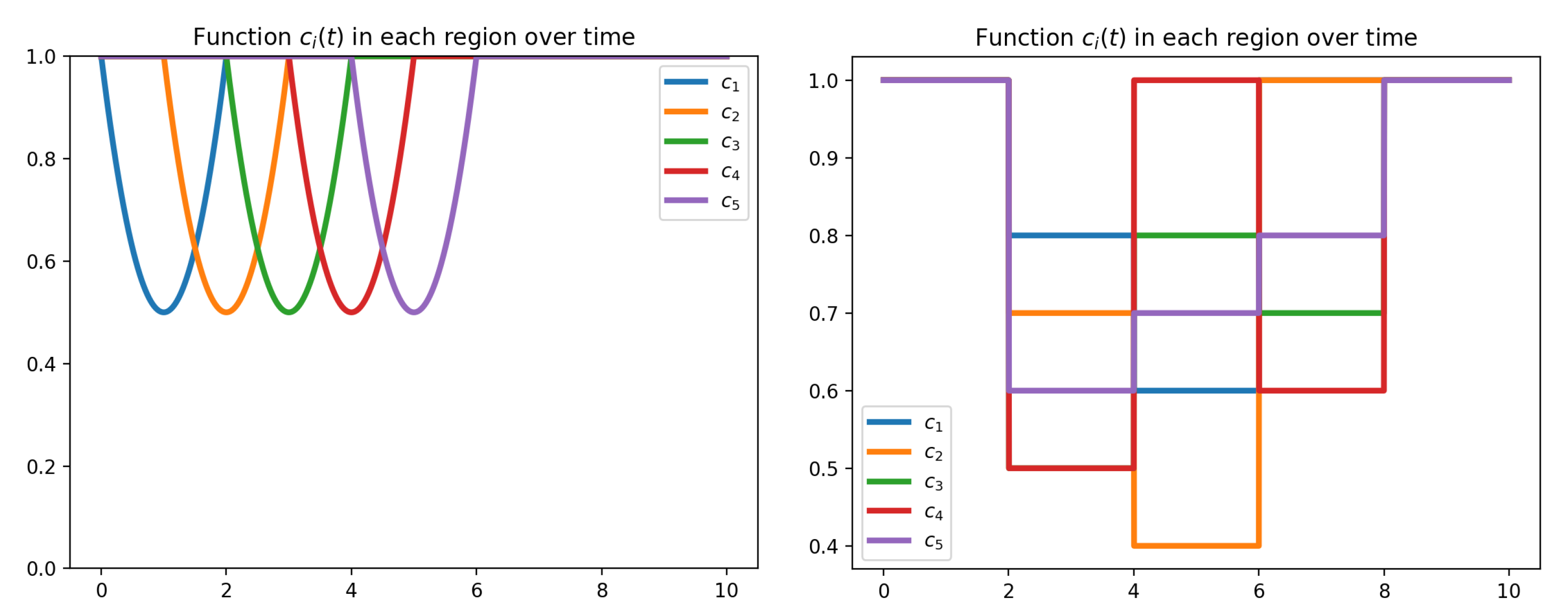
For the first example, each function
is given by
This choice of functions is represented on
Figure 1 and (in some way) models the fact that the productivity is reduced in each region gradually and then come back to normal. The effect “propagates” over time from the first region to the last one.
In the second case, we have taken the same values for
,
and
but we have changed the functions
:
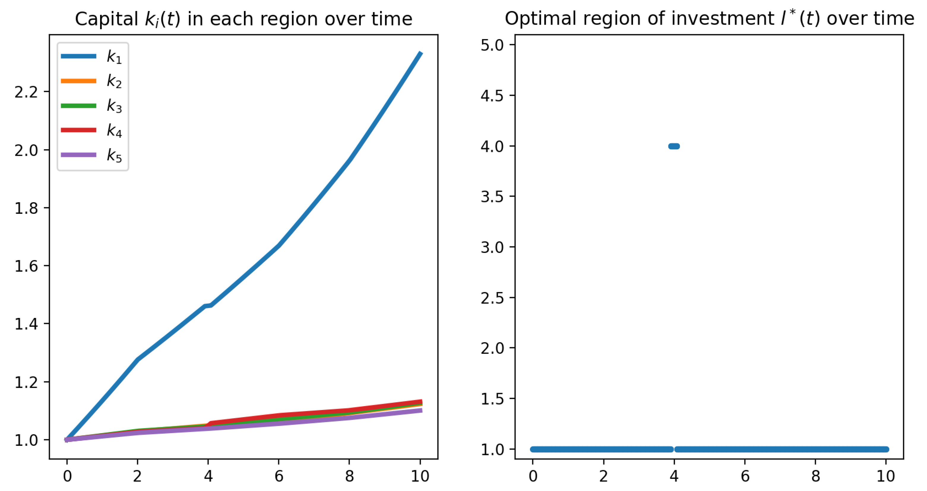
which corresponds to a situation where the effect of the lockdown is much stronger and is applied abruptly in each region.
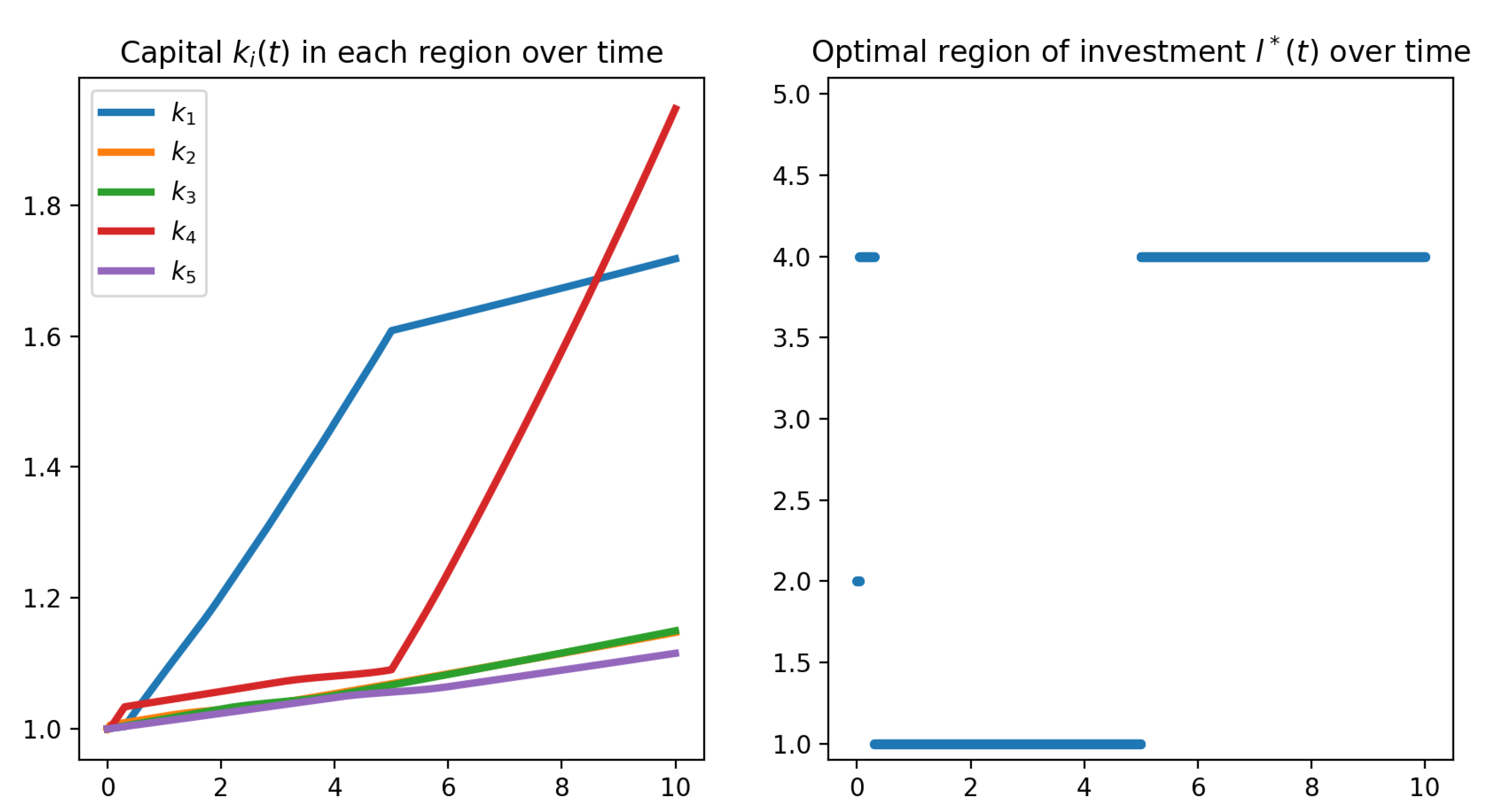
For this first example, we have represented on
Figure 2 the obtained results for
and
taking
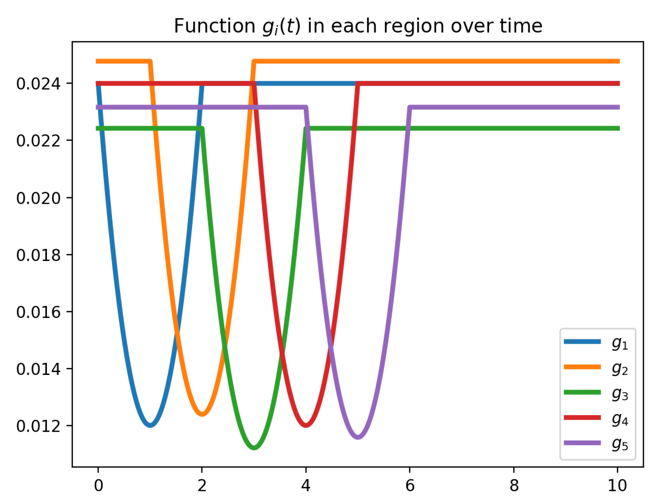
. We can see that the investment strategy is not obvious. It leads to
. Furthermore, we can show that it does not correspond to invest only in the region with the maximum rate
at time
t. Indeed,
Figure 3, where we have represented the function
, would suggest to invest first in region 2, then in region 4 and, finally, again in region 2. If we apply this strategy, we get
whereas we get
with the optimal strategy.
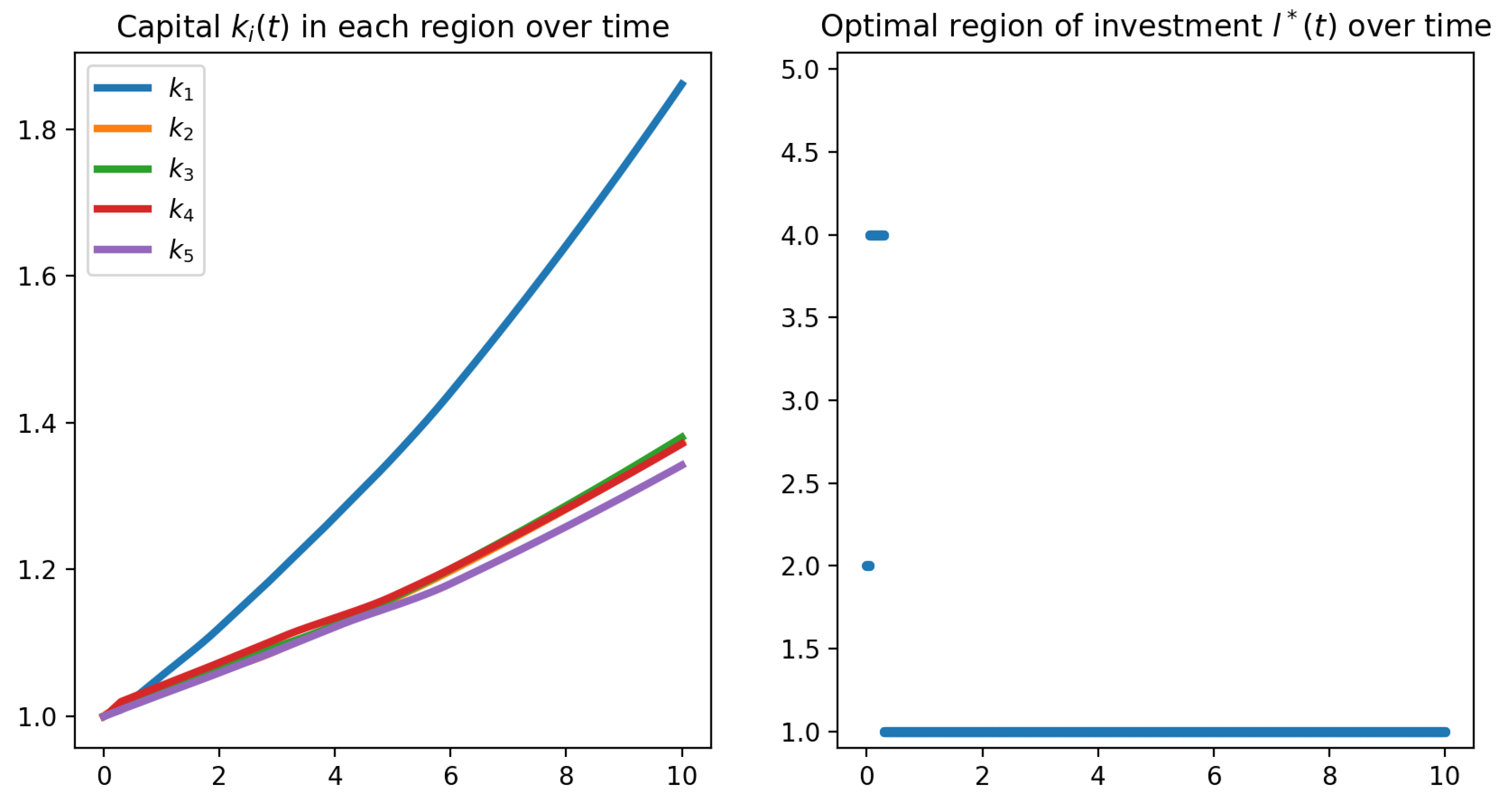
Let us now illustrate the effect of parameter
. Taking for the same example
, which we recall means that at least a part of the profit is equally distributed between regions, we obtained a different optimal strategy, as shown on
Figure 4. Furthermore, as expected, the final income
is lower than the one obtained by taking
. However, this strategy ensures that every regions receives a minimal support and it considerably reduces disparities.
For the second example, we have represented the obtained results on
Figure 5, taking
. Once again, one can see that the strategy is not obvious. Furthermore, it is clearly not the same as in the first case, for the same
, which accounts for the change of function
.
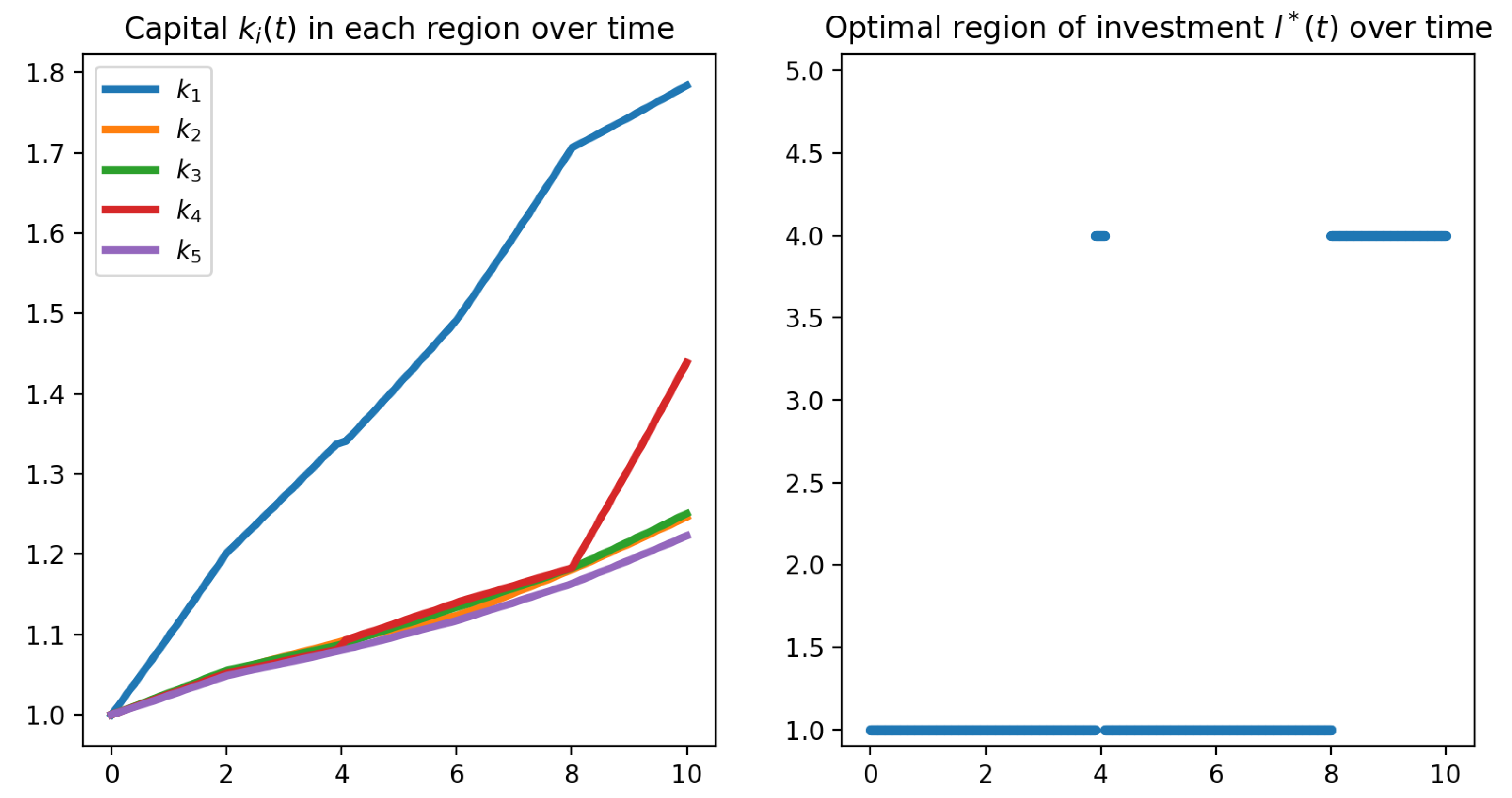
To emphasize the impact of the parameter
, we have computed the optimal strategy taking
, see
Figure 6. Here again, we can observe that the optimal strategy is changed and increasing
alleviates the disparities.
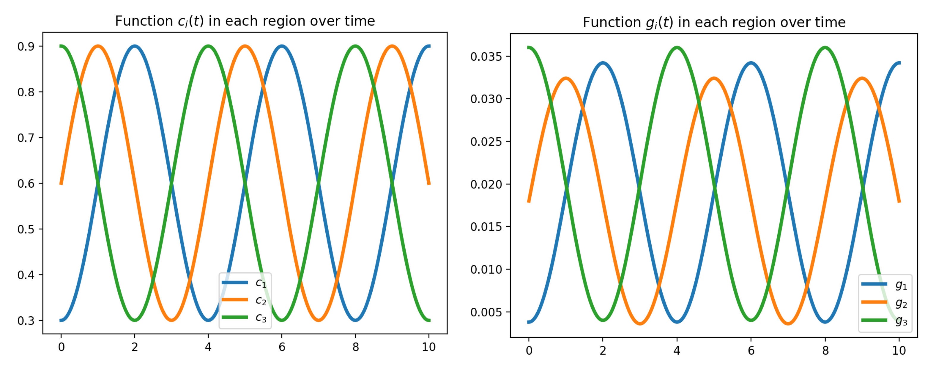
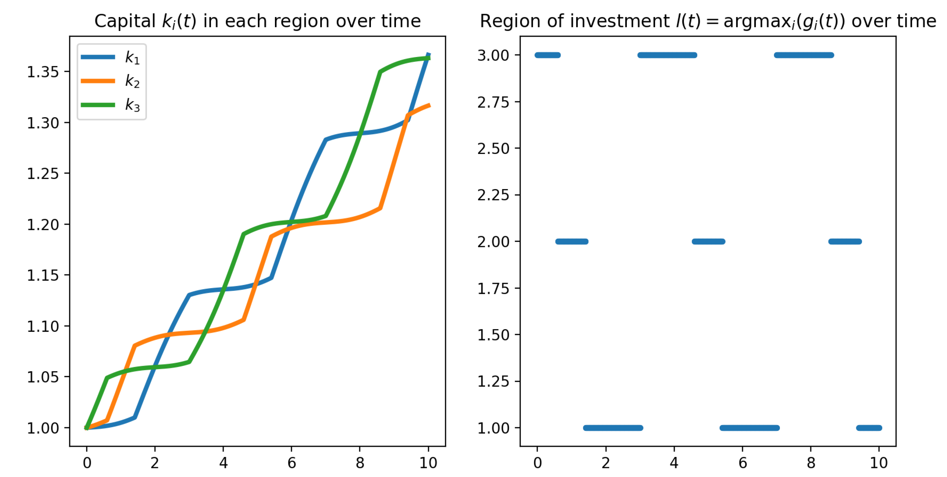
A last example modelling seasonal effect: To end this section, let us consider the case of periodic functions
. This can be interpreted as seasonal effect, for instance a region close to the sea will be more attractive in summer, whereas a region with mountains will be more attractive in winter. We have consider the case of three regions characterized by the following parameters:
The function
is represented on
Figure 7 and is given by:
These three regions can be interpreted as follows: region 1 corresponds to sea region, region 2 to countryside and region 3 to mountain region. When the sea region is more attractive (usually in summer), the mountain region is less attractive. In order to see which region has the best productivity
at each time
t, we have also represented on
Figure 7 the functions
. One can see that globally region 1 and region 3 have the highest productivity alternatively, and on a short period region 2 has the best productivity.
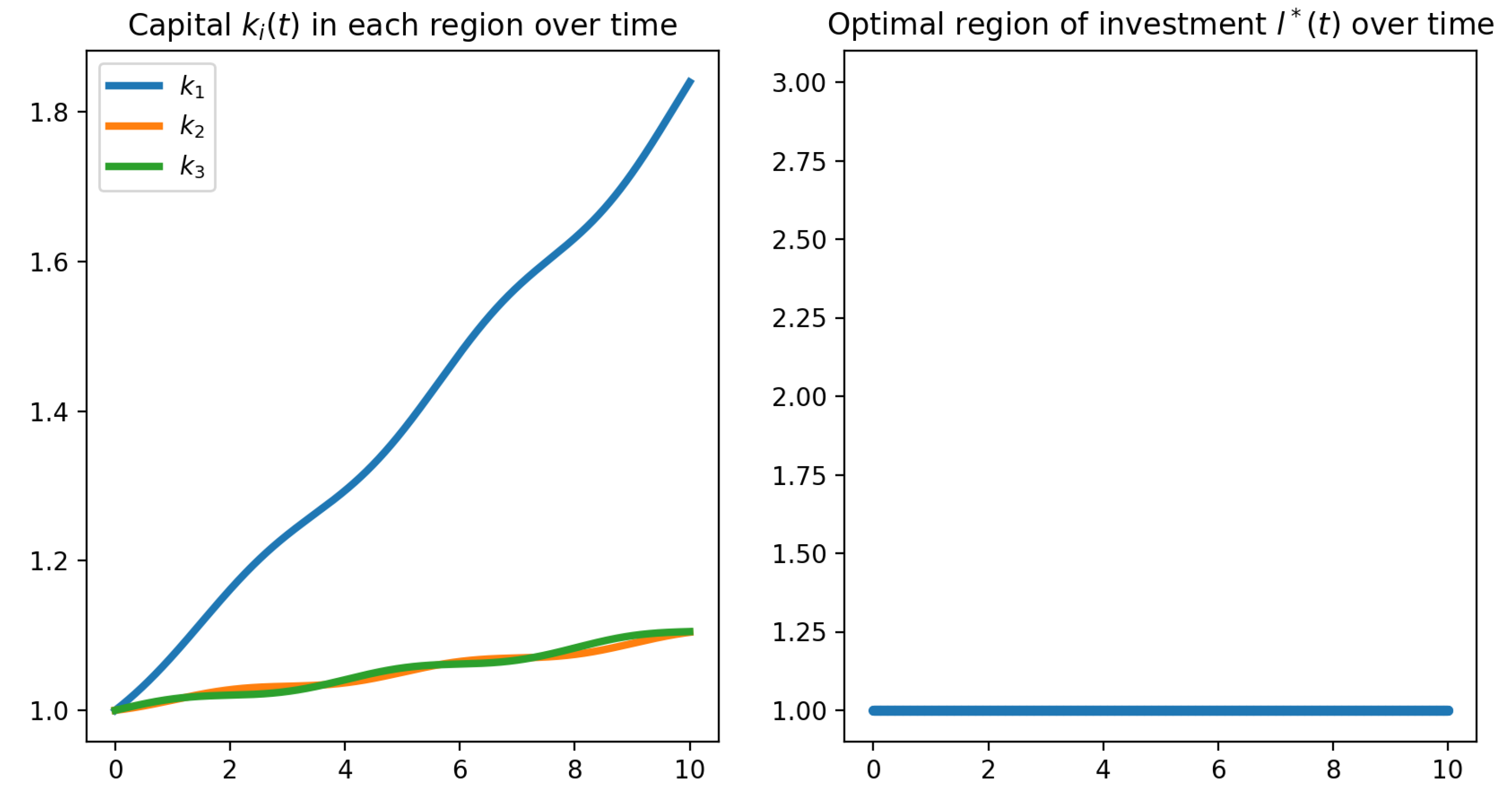
On
Figure 8, we have represented the optimal solution of our optimization problem (taking
) and, as we can see, the optimal strategy consists simply in injecting the money in the same region (region 1). In this case, the final value
.
This result might seem counter-intuitive and one could think that a better strategy consists in injecting money in the most productive region, that is to say, to take:
To compare the two strategies, we have represented on
Figure 9 the results obtained following this second strategy. In that case, the final value
is smaller than the one obtained by the optimal strategy (which is logical).
4. Conclusions and Discussion
In this work, we have proposed a mathematical model to describe the impact of a regional lockdown or seasonal effect on the economy. In particular, we have emphasized that constructing the optimal strategy is not obvious and requires numerical methods. Furthermore, one interesting feature of the proposed model is the fact that we can consider a particular policy to avoid keeping or increasing regional disparities. Clearly, if we wish to minimize the disparities and to sustain poor regions, we need to take . Yet, doing so, no strategy can be established (since we no longer have control parameters) and it can quite highly affect the final income , and also slowdown the development of other regions.
A first and direct extension of the model would be to consider a variable in time parameter instead of a constant value . Furthermore, one could consider that the part of the benefit generated by the different regions is not equally distributed among the regions. This implies to consider depending both on time and region i. These two generalisations are straightforward and do not change the analysis.
A second improvement of the model would be to consider another cost-functional, such as
where
is a function equal to
X if
and fastly decreasing when
decreases. Doing so, we would penalize the fact that a region does not reach a minimal capital
. Another improvement would be to consider an economic growth model more realistic such as logistic growth:
In this model, represents a limit capital that can be reached. Yet, these two improvements leads to much involved difficulties to solve the optimization problem.
As a final extension, let us also mention the addition of a stochastic term in the model. This term would account for random influences on the model. Considering the fact that the stochastic version of Pontryagin’s principle is different from the one used in this work, this extension would be required to fully review the analysis. The numerical part would also be quite different, since the adjoint equation would be a backward stochastic differential equation. In particular, in this future work, it would be very interesting to see the impact of a stochastic term on the optimal policy.
Regarding the usefulness of the proposed model, it can be applied both for situations of prolonged regional lockdown over longer periods, and for temporary situations due to possible natural disasters. From the point of view of managerial implications, the model can be adapted both for companies and for decision makers in the field of public policies: at zonal level (mayors, prefectures) and at regional/national level (local government, national government, ministry of finance). The model can be applied depending on the purpose pursued by the policy maker: maximizing revenues or ameliorating regional disparities.
As a future research direction, the inclusion of other parameters or restrictions in the model can be considered, adapted according to the type of lockdown or interruption of activities. For example, a set of constraints and variables that emulate situations in which all activities in a region are interrupted or only activities in a certain field of activity.


