1. Introduction
This article is devoted to the study of Boolean-valued algebraic systems of set-theoretic signature. The primary audience is assumed to be general mathematicians who are interested in the formal backgrounds of Boolean-valued analysis.
The key facts presented here are not new: The defining axioms of a Boolean-valued universe, its existence, uniqueness, and basic properties (such as the transfer, ascent, mixing and maximum principles) are well known. What is new here is a systematic study of the Boolean-valued universe as an algebraic system, with some new tools including partial elements, superstructures over extensional Boolean-valued systems, and intensional cumulative hierarchies.
The main content of the paper is divided into four sections.
Section 2, “General Formalism,” is devoted to the notion of Boolean-valued algebraic system and exposes the logical backgrounds of various useful extensions of the syntax of Boolean truth values. In
Section 3, “Basic Technique,” we present the main tools related to Boolean-valued systems (including the new apparatus of partial elements), study the key properties of the systems, and clarify interrelations between them. In
Section 4, “The Structure of the Boolean-Valued Universe,” we elaborate the notion of universe over an arbitrary extensional Boolean-valued system and present the main results on the classical universe
: existence, uniqueness, logical independence of the axioms, hierarchical structure. In
Section 5, “Applications of the Lévy Hierarchy,” we suggest a development of the technique based on the quantifier classification of formulas and demonstrate how it can improve the Boolean-valued transfer principle for the canonical embedding.
Let be the totality of all formulas of set-theoretic signature defined in the metatheory. The metaformula that defines can be rendered into the language of as a formula, , thus providing a definition, , for the set of internal formulas. The same is true of the metaset of sentences (i.e., formulas without free variables) and the set of internal sentences. In a similar manner, given an arbitrary formula , we may render into its description and thus obtain a definition, , for the set , the code of φ. This results in a conservative extension (actually, an eliminable extension; see Definition 5) of by means of the definable constants , , and such that for all , .
In all contemporary articles and textbooks devoted to Boolean-valued models of set theory, given a complete Boolean algebra
B, the truth valuation in the
B-valued universe
is described
informally either as a class function
mapping each sentence
of signature
, with elements of
regarded as constants, to an element
of
B; or as a class function
that maps each pair, constituted by a formula
with
n free variables and a tuple
, to an element
of
B; see, for example, [
1] (3.1–3.3), [
2] (Boolean-Valued Models, pp. 206–207), [
3] (Construction of the model, pp. 20–29), [
4] (2.1.6, 2.1.7), [
5] (4.1.6, 4.1.7). The informality mentioned above is twofold. First, the set
of internal formulas is implicitly meant instead of
; and, second, the class function
is actually not defined and, moreover, cannot be defined. The latter is explained as follows: In the case of
, the separated 2-valued universe
is naturally isomorphic to
, and the truth function
satisfies the condition
for all sentences
. Therefore, if
were definable, the formula
would be a truth predicate for
:
which, by Tarski’s undefinability theorem [
2] (12.7), is impossible unless
is inconsistent.
The authors are certainly aware of the informality. For instance, there is a warning in [
2] (Models of Set Theory and Relativization, pp. 161–162) that the relativization
is
not defined for
, and the satisfaction
is
not defined if
M is a proper class; and when considering models of set theory that are proper classes, due to Gödel’s Second Incompleteness Theorem, we have to be careful how the generalization is formulated. In [
3] (Construction of the model, Remark 1, p. 24) this “tiresome point” is commented as follows: “The construction of
for arbitrary
evidently has the form of a
truth definition for set theory and so cannot be completely formalized within the language of set theory... The machinery available in
is not (unless
is inconsistent) strong enough to formalize the construction of the map
as a function of . More precisely, one can prove in
that the collection of all pairs
is not a definable class. We must therefore think of this map as being defined
metalinguistically.” Furthermore, as was said in [
6], because of the “undefinability of truth” one cannot express “
holds in
for all formulas
” in a single set-theoretical formula. Usually what is in question is a scheme of theorems and there is no particular difficulty giving a correct treatment. People are sloppy about this detail but that is only to concentrate on the essentials.
In the present article, we do not avoid inessentials and do our best to give a correct treatment of all the details. We discard internal formulas, define the Boolean truth valuation “metalinguistically,” and thoroughly expose the logical backgrounds of Boolean-valued modeling. This is what
Section 2, “General Formalism,” is devoted to. In the section, we provide an accurate formal definition for the notion of Boolean-valued algebraic system and also justify the use of theoretically definable symbols, internal classes, outer terms, and external Boolean-valued classes in the truth valuation syntax.
Another subject currently lacking in the literature is the study of
as an algebraic system of set-theoretic signature. General properties of Boolean-valued systems were considered only in their connection with representation in
and with specific technical aspects of ascents and descents; see [
4] (Chapter 4), [
5] (Chapter 7). Until recently, Reference [
1] was the only publication in which the characteristic algebraic properties of
were listed; see [
1] (3.4). In
Section 3, “Basic Technique,” we methodically examine those key properties of Boolean-valued algebraic systems under the names of extensionality, regularity, intensionality, and predicativity. The main tools in this research include the new apparatus of partial elements, joins of antichains, mixings of subclasses, ascents and descents of various kinds, the use of Boolean-valued classes in the language of truth values, and the absoluteness of bounded formulas for transitive Boolean-valued subsystems. We also introduce and study
-regular Boolean-valued systems, examine the maximum principle, and analyze its relationship with the ascent and mixing principles.
The axiomatic characterization of the Boolean-valued universe presented in [
1] (3.4) became the main motivation for our research; and the primary aim was to develop approaches to proving the uniqueness assertion claimed therein (see Definition 55 and Theorem 15). Furthermore, Professor Robert M. Solovay noted in [
6] that all the axioms listed in [
1] (3.4) were needed for a complete description of the
B-valued universe, and the examples for this could be given in the special case of
. For instance, to justify the necessity of regularity, one could build up a universe not from the empty set but from a non-well-founded collection. Therefore, we aimed at proving that the five conditions (a)–(e) of Definition 55 listed in the axiomatic characterization of
are logically independent, and, moreover, we aimed to do that for all complete Boolean algebras
B. To this end, we elaborated the notion of universe over an arbitrary extensional Boolean-valued system and established a close interrelation between such a universe and the intensional hierarchy, a Boolean-valued analog of the von Neumann cumulative hierarchy. This general tool, presented in
Section 4, “The Structure of the Boolean-Valued Universe,” makes our aims easily achievable (Theorem 15 and Examples 1–5). As a bonus, we obtain the descriptions of
by means of four cumulative hierarchies (see
Section 4.3).
Another bonus can be derived from the formalism of eliminable extensions exposed in
Section 2.2. As soon as we know the logical backgrounds of formal definitions, we can analyze the structure of the low-level set-theoretic translations of definable mathematical objects and properties. In certain cases, this knowledge can considerably simplify verification of the validity of complex assertions inside the Boolean-valued universe. As is known (see [
4] (2.2.9), [
5] (4.2.9)), if an assertion
about sets
belongs to class
, that is, can be expressed by a set-theoretic formula
with all quantifiers in
having the form
or
; then
implies the validity of
inside
for every complete Boolean algebra
B. In
Section 5, “Applications of the Lévy Hierarchy,” we suggest some additions to the set of tools which help to successively build more and more complex formulas and terms, while staying within the class of
constructions. As an example, we demonstrate that the use of the tools can shorten the proof of the validity
from a couple of pages to a couple of lines (see
Section 5.4). We also analyze the logical structure of several classical definitions of the field of reals and find out which of them guarantee the inclusion
inside
for all
B.
2. General Formalism
Since the primary audience is not assumed to consist of specialists in logic or formal languages, we consider it appropriate to start the exposition with describing the logical machinery of formal definitions, utilization of classes in set theory, and the use of infinite assertions in implications. In this section, we present the basic information related to the notion of Boolean-valued algebraic system and formalize the use of definable symbols, outer terms and external Boolean-valued classes in the syntax of Boolean truth values.
2.1. Logical Prerequisites
As a logical base we use the classical Hilbert-style first-order predicate calculus with equality. Therefore, throughout the article, we assume that, first, all signatures under consideration contain the binary predicate symbol “=” and, second, the axioms of the calculus include the standard axioms of equality.
Definition 1. Let Σ be a signature. (The signature can be infinite but is always assumed at most countable and decidable.) By a theory (more exactly, an axiomatizable theory) of signature Σ we mean an arbitrary decidable subset of the set of formulas of signature Σ. The elements of are called the special axioms (or nonlogical axioms) of the theory. Given a formula , the expression means that φ is a theorem of , that is, φ is deducible from the axioms of the predicate calculus of signature Σ with equality and the special axioms of by means of the classical deduction rules. If is a set of formulas, we write whenever for all . The expression serves as a shorthand for and thus means that φ is provable in the calculus of signature Σ without any special axioms. Due to the Soundness and Completeness theorems, a formula φ meets if and only if φ is a tautology of signature Σ, that is, φ is true in every algebraic system of signature Σ with the standard interpretation of equality. Formulas φ and ψ subject to are called logically equivalent.
Definition 2. The variables with free occurrences in a formula or term are called the parameters of the latter. The parameters of a set of formulas or terms are the variables contained in the union of the parameters of formulas and terms in the set. Formulas and terms having no parameters are called closed; closed formulas are also called sentences. If is the complete list of parameters of a formula φ, then the closed formula is called the universal closure of φ and denoted by . Given a set of formulas, put .
Definition 3. Expressions of the form or are used to denote arbitrary finite lists of variables or terms. The cardinality n of a list is denoted by . The formulasare abbreviated as , , and . Agreement 1. We assume that the set of all variables is computably organized into a sequence and call the corresponding order the alphabetical order. By saying “ is a formulawith parameters ” or “ arethe parameters of ” we always mean that is the complete list of parameters of listed without duplicates in the alphabetical order. By the parameters of a finite set of formulas we mean the union of their parameters listed without duplicates in the alphabetical order. The same is true of the parameters of terms and of finite sets of terms.
Agreement 2. In what follows, the words “a new variable” or “new variables” stand for the alphabetically first variables that do not occur in the preceding formulas or terms under consideration. This agreement is necessary for making the constructions well-defined and keeping the procedures computable (see, for instance, Definition 7(d) and Definition 21).
We make a conventional agreement that simplifies the syntax of term substitution.
Agreement 3. When writing a formula initially as , with presupposed to be pairwise different variables, we do not assume that all the variables participate in as parameters. We also do not assume that all the parameters of belong to the list . The initial notation only means that every subsequent expression of the form denotes the result of simultaneous substitution of the terms in for (with possible name collisions eliminated by renaming the bound variables of occurred in ). If are not among the parameters of , then the formula is logically equivalent towhile in the general case we havewhereare new variables Agreement 2).
The analogous agreement is proposed about the notation of the form and its relation to the result of simultaneous substitution of the terms in the term for .
Definition 4. In what follows, is the set of naturals; is the least infinite ordinal. The class of all ordinals is denoted by ; and the class of all limit ordinals, by . Moreover, we use the notationwhere and for all . The symbol “⊂” stands for the non-strict inclusion. 2.2. Eliminable Extensions
After examining several examples of definitions, we formalize the notion of definition as an eliminable extension of a theory; present a useful criterion for the eliminability of an extension; clarify the notions of correct and conditionally correct definition; list the key properties of an elimination of definable symbols; and justify iterative definitions and the union of independent definitions.
We start with a brief description of a possible formalism behind introduction of new notation and terminology, that is, extension of the language of a theory by means of definitions of new formulas and terms, such as , , , , ⌀, .
The role of the formal language of set theory is conventionally played by the first-order predicate language of formulas of signature . Initially, the language consists of the atomic formulas and (with x and y arbitrary variables) and the formulas recursively constructed from simpler formulas by means of propositional and quantifier connectives.
Suppose that we would like to extend the language of set theory with the new formula and the two new terms and ⌀. To this end, it suffices to consider the signature that enriches with the binary predicate symbol ⊂, unary function symbol , and constant ⌀. As a result, the formal language of the extended signature contains such new atomic formulas as , , and so forth, as well as various formulas recursively constructed from the new formulas, including, for instance, the formula that literally belongs to the extended language and does not contain any abbreviations or informal notation.
By enriching the signature
to
we extended the language with some new expressions but did not make them “sensible.” The task can be performed by adding axioms that play the role of the corresponding
definitions. Consider the formulas
and denote by
the theory of signature
obtained from
by adding the following three special axioms:
Since the formulas
,
, and
belong to the language of signature
, every formula
of the extended language
admits a “translation” into the initial language
, an equivalent formula
of signature
. The translation procedure can be organized recursively by passing through the logical connectives and transforming the atomic formulas of signature
according to the above definitions:
where
x and
y are variables;
and
are terms of signature
;
and
are formulas of signature
.
It is important to note that the formulas and are provable in , which guarantees the correctness of the definitions introduced: formal reasoning within the extended theory belongs to legal deduction means, that is, the use of definitions does not make it possible to prove anything unprovable in the pure .
Definition 5. Guided by the above example, we may conclude that a definition, or an introduction of new notation, is a conservative extension of the theory which admits elimination, “restatement” of the assertions of the extended language in terms of the initial language.
Consider a theory of signature Σ. An eliminable extension of , or an extension of by means of definitions, is an extension of to a theory of a richer signature subject to the following conditions:
- (a)
is a conservative extension of , that is, implies for each ;
- (b)
for each there exists such that.
(Analogs of the notion of eliminable extension can be found in the literature under the name of definitional or inessential extension.) The special axioms ofthat do not belong toare called the definitions or the defining axioms; the formula ψ in (b) can be called a translation of φ into the language of Σ or a restatement of φ in terms of Σ.
Observe that the set of new symbols can be infinite (see, e.g., Definitions 6 and 11). Nevertheless, due to the requirement that the signatures and the sets of axioms are decidable (see Definition 1), each eliminable extension admits an elimination in the form of a computable functionmapping each formula φ of signature to a formula of signature Σ so that We present a criterion for the eliminability of an extension that is easily verifiable for the majority of definitions occurred in mathematical practice.
Theorem 1. Let be a signature that enriches a signature Σ by a set P of new predicate symbols and by a set F of new function symbols, and let be a theory of signature that extends a theory of signature Σ. The theory is an eliminable extension of if and only if there is a function mapping the symbols to formulas of signature Σ so thatwhere is the theory obtained from by adding the special axioms Proof. Sufficiency: The conservativity of the extension can be easily verified with the help of the Soundness and Completeness theorems. An elimination for can be defined by starting with the elimination available for the atomic formulas and then recursively extending it to all formulas by preserving the logical connectives.
Necessity: Given and , put and , where is an elimination of the extension . We only need to verify the condition . Consider an arbitrary . The above-proven “sufficiency” implies that the extension admits an elimination . Since , , and ; we have and so . Taking account of , we successively deduce , , , , . □
Agreement 4. The conditionin Theorem 1 is conventionally called the correctness of the definition .
(If the correctness is violated, the extensionof a consistent theoryfails to be conservative.) Nevertheless, mathematical practice is replete with examples of termsbeing correctly defined only under certain conditionson the parameters:
Such a conditionally correct definition can always be made correct by lettingin the case of:
The above modification is implicitly assumed to be applied to each conditionally correct definition.
Agreement 5. As is easily seen, every eliminationof an eliminable extensiontranslates formulas of the initial language to equivalent formulas:for all. The elimination is also invariant with respect to the logical connectives:and so forth. Moreover, the translation procedure can always be reorganized so that
- (a)
the initial formulas are unchanged:for all;
- (b)
the logical connectives are preserved:
, , , etc.;
- (c)
each formulais translated to a formulawith the same parameters.
In what follows, we assume that every elimination under consideration possesses the above-listed properties (a)–(c).
Due to property (b), the translation of a formula does not depend on the context in which the formula is contained in superformulas. We thus may regard any formula of the extended signature as a synonym (denotation, shorthand) for its translation into the initial language of and handle the new formulas so as if they belong to the formal language of the basic theory under consideration.
Remark 1. If is an eliminable extension of , and is an eliminable extension of , then is an eliminable extension of . This trivial observation justifies iterative definitions of new symbols by means of those previously defined.
Remark 2. Let be a theory of signature Σ, and let and be eliminable extensions of of signatures and , with . Then the theory of signature is an eliminable extension of (cp. [7] (Theorem 20.6)). This justifies correctness of the union of independent systems of definitions. 2.3. Classes in Set Theory
After introducing the syntax of subclasses of sets as an eliminable extension, we will formalize the extension of the language of set theory by arbitrary definable, or internal, classes with the aid of so-called syntactic sugar.
Definition 6. In order to demonstrate an eliminable extension of with infinite set of new signature symbols, we will formalize the enrichment of the language of set theory by terms of the form .
Let x and y be different variables and let be a formula, where is the alphabetically ordered list of all parameters of φ other than x and y. For each triple described above, enrich the signature of set theory by the function symbol of arity , introduce the abbreviationand add the defining axiomDue to the obvious provability of the equality(with v and arbitrary variables, and u a variable different from ), we can avoid using the general expressions of the form and confine ourselves to the use of the terms . Remark 3. Since the new symbols were introduced for the language whose signature had not contained those symbols, the language has not been enriched by expressions of the formThis restriction can be removed, for instance, by the union of the sequence of extensions, each of which enlarges the admissible nesting depth of the new constructions in each other. The corresponding procedure can be called the grammatical closure (cp. (1)). The formalism of eliminable extensions described in Definition 5 does not allow us to enrich the language of by the terms of arbitrary definable classes and, in particular, by the terms and . (No consistent extension of can provide the theorem for a term , since the formula is deducible in the predicate calculus.) Similarly to the case of eliminable extension, extension of the language by the syntax of definable classes assumes enrichment of the signature by new symbols; but the theory per se is not extended, and the role of elimination is played by the so-called syntactic sugar, an explicit translation procedure of the formulas of the extended language into the language of the initial signature.
In this subsection, when writing a formula as , agree to suppose that is the complete list of parameters of other than x, while x need not participate in .
Definition 7. Let Σ be an arbitrary signature. For each pair , with x a variable and a formula of signature Σ, consider the function symbol of arity and introduce the notation for the term :The symbols are called class symbols, and the terms are classes or, more exactly, definable classes or internal classes. Denote by the signature obtained from Σ by adding the class symbols , with . Let be the smallest enrichment of the standard set-theoretic signature that is closed under the formation of classes:There exists a unique mapping subject to the following conditions: - (a)
is identical on , that is, for the formulas φ of signature ϵ;
- (b)
preserves the logical connectives, that is,
, , , etc.;
- (c)
for all variables x and y, all formulas of signature , and all terms of signature , - (d)
for each variable x and all terms of signature that are not variables,where u is a new variable (see Agreement 2).
The mapping is called the elimination of classes.
Say that terms σ and τ of signature are syntactically equivalent and write , whenever σ and τ are interchangeable without affecting the result of elimination, that is, for every formula φ of signature and every variable x. From condition (d) it is clear that the equivalence amounts to the equality , where u is not a parameter of τ or σ. Moreover, if is a formula of signature , are terms of signature , and ; then, according to (c), we haveand, consequently,Therefore, every term of signature is syntactically equivalent to a suitable class, and so we may refuse to employ expressions of the form and confine ourselves to the use of classes without decreasing the expressive power of the language (cp. Definition 6). The parameters of a class are the parameters of the class as a term of signature , which evidently coincide with the parameters of φ other than x. For instance, if the formula of signature ϵ expresses the containment of a set x to the classical B-valued universe, then the termof signature is a class with parameter B. Remark 4. Due to Definition 7, the language of each theory of set-theoretic signature ϵ can be extended by the use of classes. Moreover, the extension is purely syntactic and has no relation to the theory. The enrichment of the signature is not accompanied by any extension of the axiomatics. In particular, classes do not become terms of the theory under consideration, and the logical axioms remain corresponding to the predicate calculus of the initial signature ϵ. (For instance, if x and y are variables, C is a class, and the theory does not contain the axiom of extensionality, then the formula needs not to be a theorem.) In this respect, formulas of signature are not full-fledged participants of the theory and, due to the syntactic sugar, are regarded as synonyms (denotations, shorthands) for the results of elimination of classes applied to them.
Conditions (a)–(d) of Definition 7 determine the elimination of classes only for the formulas of signature and are not applicable to any extension by means of definitions. If classes are used in the language of an eliminable extension, then, for translating a formula into the initial language of signature ϵ, we should, first, apply an elimination of the extension (in order to obtain a formula of signature ) and, next, eliminate the classes.
Agreement 6. Terms are conventionally regarded as particular cases of classes, since every eliminable extension of proves the equality for each term (whose parameters do not include x). Therefore, when calling any symbol X a class, we do not exclude the case in which X is a variable or a term definable by an eliminable extension of.
The above agreement does not mean replacement of set theory by any theory of classes and does not extend the language of formulas by quantifiers over classes. Even if a symbol X is chosen to mean a class , the expression , which is a shorthand for the formula , is interpreted as existence of a set (not a class) possessing the property .
The phrases “for all classes” and “there exists a class” are meta-quantifiers. The corresponding statements usually produce infinite assertions (see
Section 2.4 below) and are formalized on the meta-theoretical level. For instance, if
and
are formulas, and the statement
is asserted to be a theorem of
, then the conjunction of the following two meta-assertions is actually meant:
- (a)
for an arbitrary class X, there is a class Y such that ;
- (b)
for arbitrary classes X and Y, .
Definition 8. If X is a class, then the phrase “X is a set” means the formula or, more exactly, . (Here y is not a parameter of X.) The negation formalizes the phrase “X is a proper class.”
2.4. Infinite Assertions
Infinite assertions are specific for the subject under consideration. Those are infinite sets of formulas. For instance, the assertion “ is valid for all classes X” is constituted by all the formulas , with x a variable and an arbitrary formula. The examples of infinite assertions are also “X is a model of ” (see Proposition8) and “X meets the maximum principle” (see Definition 43).
Mathematical texts often use “declarations of hypotheses.” Such a declaration means that, within a fragment of reasoning, certain conditions are assumed to be valid or some variables are fixed and play the role of objects with certain properties. As an example serves the phrase “in what follows, B is a complete Boolean algebra” that the next subsection of this article starts with. Actually, the phrase fixes the letter B and adds a temporary axiom that formalizes the assertion “B is a complete Boolean algebra.”
In most cases, the effect of declaring a hypothesis is quite clear at the informal level, but the use of infinite sets of formulas as hypotheses or conclusions requires accuracy.
Logical connectives with infinite assertions make sense due to the apparatus of formal deduction. For instance, if at least one of the assertions or is infinite, then the implication itself has no sense; while the phrase “ implies within the theory ” can be formalized as , that is the deducibility of from the hypotheses within .
Definition 9. Let be a theory of signature Σ and let Γ and Δ be arbitrary sets of formulas of signature Σ. (The sets Γ and Δ can be infinite and may have parameters.) Assume that the formulas in Δ do not contain quantifiers over any parameters of Γ. The deducibility of the conclusion Δ from the hypothesis Γ within is written as and defined by means of the notion of formal deduction in predicate calculus: For every formula there is a finite sequence of formulas such that and each formula either belongs to or is obtained from the previous formulas by one of the classical deduction rules save the rules with quantifiers over the parameters of Γ. Informally, the latter means that the parameters of the hypothesis are fixed and play the role of constants (cp. Proposition 3).
The propositions presented in this subsection are well known and can be easily verified by using the Soundness, Deduction, and Completeness theorems.
Proposition 1. Let be a theory of signature Σ and let Γ and Δ be arbitrary sets of formulas of signature Σ such that the parameters of Γ are not quantified in Δ. Then the following are equivalent:
- (a)
;
- (b)
for all ;
- (c)
for every there is a finite subset such that or, which is the same, ;
- (d)
for every model X of and every valuation of the parameters V of , the validity of all implies the validity of all .
Proposition 2. Let be a theory of signature Σ and let Γ be an arbitrary set of formulas of signature Σ. Suppose thatfor every finite subset with parameters . Then Γ conservatively complements in the following sense:whenever φ is a formula of signature Σ and the parameters of Γ do not occur in φ. Another approach to a formalization of a decidable set of hypotheses consists in replacing the parameters of with new constants and extending the theory with regarded as an additional set of axioms. After discarding the hypotheses in this way, we can use the standard deduction in the extended theory.
Proposition 3. Let be a theory of signature Σ, let Γ be a decidable set of formulas of signature Σ, and let be the (finite or infinite) set of all parameters of Γ. Consider the signature obtained from Σ by adding the set of new constants. Given a formula φ of signature Σ, denote by the result of substituting the constants for the free variables in φ. Let be the theory of signature obtained from by adding the set of axioms .
- (a)
If δ is a formula of signature Σ without quantifiers over V, then the deducibility is equivalent to .
- (b)
If for every finite subset with parameters , then is a conservative extension of .
Declaration of a finite set of hypotheses obviously reduces to the case of a single hypothesis and admits a simpler formalization based on the following fact.
Proposition 4. Let be a theory of signature Σ and let be a formula of signature Σ with parameters . Consider the signature obtained from Σ by adding the constants and let be the theory of signature obtained from by adding the axiom .
- (a)
For every formula of signature Σ without quantifiers over , - (b)
If then is a conservative extension of .
For instance, under the hypothesis “
B is a complete Boolean algebra,” the expression
which symbolizes the provability in
of the infinite assertion “
is a model of
,” is formally equivalent to the deducibility
the latter in turn means that, for every sentence
that is a theorem of
, the following equivalent conditions hold:
- (a)
;
- (b)
;
- (c)
,
where is the conservative extension of obtained by adding the constant B and the axiom “B is a complete Boolean algebra.”
2.5. Boolean-Valued Algebraic Systems
In this subsection, we formalize the notion of Boolean-valued algebraic system, indicate the main syntactic properties of the Boolean truth valuation, and recall the basic notions related to Boolean-valued systems: extensional function, Boolean-valued class, model of a theory, separated system, subsystem, isomorphism.
Throughout the rest of the article we argue within . In particular, all the lemmas, propositions, and theorems are assumed to be stated and proven in . When introducing any definitions, declaring any hypotheses with parameters, or using internal classes, we implicitly enrich the signature and conservatively extend the axiomatics of the theory, but conventionally preserve the name of for the extended theory and identify the formulas of the extended language with the formulas of the initial language obtained by the corresponding eliminations.
In what follows, B is a complete Boolean algebra.
Definition 10. By saying that X is a B-presystem of signature Σ, we mean that
- (a)
X is a class;
- (b)
Σ is a predicative signature, that is, a signature that consists of only predicate symbols;
- (c)
a computable function is defined that maps symbols to classes ;
- (d)
and for each n-ary predicate symbol .
The class functions are called the B-valued interpretations of the symbols .
Assertion (d), that is infinite in case
is infinite, is assumed to be appended to
as a hypothesis whose parameters are
B and the optional parameters of
X and
; see
Section 2.4.
Definition 11. Given a B-presystem X of signature Σ, define the truth values of formulas φ along the lines of Definition 6. Namely, for each formula φ of signature Σ with parameters , introduce the function symbol of arity , agree to write the term as , and extend the theory by the definitionsfor all variables x, , predicate symbols , and formulas φ, ψ of signature Σ, where is the complement operation in B. The above definitions are conditionally correct (see Agreement 4) provided that the parameters of the formulas under consideration belong to X. Equalities (2) correctly define the function symbols
within
under the hypothesis “
X is a
B-presystem.” According to Definition 5 and
Section 2.4, the definitions lead to a conservative extension of
that proves
for each formula
of signature
.
Strictly speaking, the parameters of the term are not only those of the formula , but also the parameters of the hypotheses declared in the definition of Boolean truth values (including the variable B and the optional parameters of the classes X and ). Nevertheless, with account taken of Propositions 3 or 4, the parameters of hypotheses can be regarded as constants and excluded from the arguments of the function symbols .
Lemma 1. Let X be a B-presystem of signature Σ, let be a formula of signature Σ with parameters , and let be an arbitrary list of variables with . Then (the extension of) proves that, for all ,
- (a)
;
- (b)
.
Proof. (a): Consider the case of an atomic formula,
, with
. According to definitions (2), for all
we have
,
, and, consequently,
The case of a complex formula
is easily proven by induction on the complexity.
(b): no symbols: Due to equality (a) we have
From equality (b) it follows that the expressive power of the language will not decrease if we refuse to employ expressions of the form and confine ourselves to the use of terms (cp. Definitions 6 and 7).
Definition 12. Let X be a B-presystem of signature Σ and let be a formula of signature Σ with parameters . On assuming , say that is valid in X and writeprovided that . Given a set of sentences of signature Σ, say that is valid in X and write whenever for all . Remark 5. Since the article is devoted to the study of Boolean-valued systems of set-theoretic signature (that is constituted by predicate symbols only), we considered it appropriate to simplify the exposition by excluding function symbols from Definitions 10 and 11. It is worth noting that the traditional approach, in which n-ary function symbols f in a system X are interpreted by functions , is not the most general solution in the Boolean-valued case. Indeed, in this approach, for all , the conditionis fulfilled in a considerably stronger form,which automatically provides the maximum principle for the formula (see Definition 43). A less restrictive approach consists in considering a predicate symbol of arity with interpretation subject toand then employing the eliminable extension in which the function symbol f is defined via by the axiomAnyway, such a generalization is unnecessary for the present article. Definition 13. Let X be a B-presystem of a signature with equality. Say that is a B-model of equality if for all or, which is the same, the axioms of equality for signature are valid in X: Let be a B-model of equality.
Proposition 5. The following properties of a function are equivalent:
- (a)
for all ;
- (b)
for all ;
- (c)
for all , ;
- (d)
for all , where .
Definition 14. A function subject to each of the equivalent conditions (a)–(d) of Proposition
5 is called extensional; see [1] (3.5), [4] (2.5.5), [5] (4.5.6). Say that a function is extensional if Φ is extensional in every of the n arguments, which is equivalent to each of the following four conditions (see Definition 3):for all , , . Extensional functions are also called Boolean-valued classes in X (see [1] (3.5), [4] (2.5.8), [5] (4.6.1)) and are employed in the language of truth values in a manner similar to the use of classes in the language of set theory (see Definition 22 below). In the sequel, the assertion that is a Boolean-valued class (i.e., Φ is extensional) will be written as .
Let be a predicative signature with equality.
Proposition 6. The following properties of a B-presystem X of signature Σ are equivalent:
- (a)
is a B-model of equality and the interpretations of all the symbols are extensional;
- (b)
the axioms of equality for signature Σ are valid in X: - (c)
for each axiom φ of predicate calculus of signature Σ (with equality);
- (d)
for all formulas φ deducible in predicate calculus of signature Σ;
- (e)
all closed tautologies of signature Σ are valid in X.
Whenever the equivalent conditions (a)–(e) hold, say that X is a Boolean-valued (more exactly, B-valued) algebraic system of signature . We will also use the shorter synonyms: Boolean-valued system and B-system of signature .
The following simple consequence of condition (d) will be often used without explicit reference:
Proposition 7. Let X be a B-system of signature Σ and let φ be a formula of signature Σ with parameters . Then the following function is extensional: As is known, the deduction rules preserve validity in any Boolean-valued system. More exactly, the following holds:
Proposition 8. Let X be a B-system of signature Σ and let Γ and Δ be some sets of sentences of signature Σ.
- (a)
If then .
- (b)
If and then .
Therefore, if is the totality of all theorems of a theory , the assertions and are equivalent. In each of the cases we call X a Boolean-valued model (or a B-model) of and write . Assertions (c) and (d) of Proposition 6
correspond to the case and state that every B-system is a Boolean-valued model of predicate calculus.
Definition 15. Let X be a B-system of signature Σ. Consider the following equivalence ∼ on X:The system X is called separated if for all . In the case of a 2-system, where is the simplest Boolean algebra; X is separated whenever the interpretation of equality in X is standard: . The quotient (see [4] (2.5), [5] (4.5)) is a separated B-system that is elementary equivalent to the initial system: for every sentence φ of signature Σ. Moreover, for each formula φ of signature Σ with parameters , we havewhenever and are the cosets of . Definition 16. Given a B-system X of signature Σ, a B-system Y is called a subsystem of X if and for all .
Definition 17. Say that a class f is an isomorphism between B-systems X and Y of signature Σ and write , if f is a bijection between X and Y subject to the conditionfor each n-ary symbol . As is easily seen, if φ is a formula of signature Σ with parameters , then impliesSay that B-systems X and Y are isomorphic and write whenever for some class f. 2.6. Eliminable Extensions in Truth Values
According to 11, given a Boolean-valued model X of set theory, the terms make sense for formulas of signature but not for formulas containing any additional definable predicate or function symbols. In this subsection, we discuss and justify the convenient use of such expressions as , , or . We also formalize the use of outer terms in the language of truth values by means of an eliminable extension that makes it possible to delegate the semantics of a term to the outer theory and legalizes the expressions of the form , with a term defined in , even for the case in which X is not a model of set theory.
Definition 18. Let X be a B-system of signature Σ, let be a theory of signature Σ, let be an eliminable extension of of an arbitrary (not necessarily predicative) signature , and let be the corresponding elimination (see Agreement 5). Acting in a similar way to Definition 11, for each formula with parameters , enrich the signature of by the new function symbol of arity , introduce the notation , and add the defining axiomto . Note that the extended syntax of Boolean truth values remains invariant with respect to the logical connectives: the equalities (2) occur provable for the formulas φ, ψ of the enriched signature . The validity in X for the new formulas φ of signature is defined by the conventional relation .
The corresponding grammatical closure (cp. Remark 3) enriches the language by terms of the form and thus makes it possible to consider Boolean-valued models inside Boolean-valued models (see, e.g., [1]). Definition 18 makes it possible to regard every Boolean-valued model of a theory as a model of an arbitrary eliminable extension of . Namely, the following holds:
Proposition 9. Let X be a B-model of a theory of signature Σ, and let be an eliminable extension of of signature .
- (a)
The system X is a model of in the sense that for each theorem φ of .
- (b)
If the signature is predicative, then the truth value of every formula coincides with its truth value in the class X regarded as a B-valued system of signature with interpretations
Moreover, .
Remark 6. The field of reals is often defined as an arbitrary Dedekind-complete totally ordered field. In , such an ordered field is unique up to isomorphism, but not unique; therefore, the corresponding definition of the constant does not meet the conditions of Definition 5. In more detail, let be a formalization, in the language of , of the assertion “xis a Dedekind-complete totally ordered field,” and let be the extension of by the constant and the axiom .
Proposition 10. If is consistent, then the extension is not eliminable.
Proof. It suffices to observe that the formula cannot be eliminated. Indeed, if there was a formula of signature such that , then we would have and, in particular, , which is not the case. □
However, due to the provability of
in
, the theory
occurs a conservative extension of
. Moreover, the extension
admits an elimination in the following weaker sense: every formula
of signature
can be computably associated with a formula
of signature
such that
The role of
can be played by the implication
, where
is the result of replacing all occurrences of the constant
in
with a new variable
r.
Therefore, the definition of the constant
as “an arbitrary Dedekind-complete totally ordered field” is formalized by a conservative but not eliminable extension. The lack of elimination complicates modeling the extension in a Boolean-valued model
X of
(see Definition 18). In the case under consideration, instead of embedding the constant
inside the syntax of
, the symbol
is introduced as “an arbitrary element of
X that is a Dedekind-complete totally ordered field inside
X.” This approach is formalized by adding the constant
and the axiom
The resultant theory occurs again a conservative but not eliminable extension of
.
Remark 7. The constant becomes eliminable if we choose a “concrete” definition of the ordered field of reals (for instance, as the set of decimal fractions or continued fractions, or as the set of cosets of Cauchy sequences, etc.), that is, a description that provides the uniqueness of the object under definition.
For example, let be a formalization, in the language of , of the assertion that x is the set of all Dedekind cuts. Employing the formalism of Definition 5, define the constant by the axiom . The symbol now becomes an element of the formal language of the extended theory. Since , the resultant extension is eliminable (see Theorem 1), and we now have the possibility of extending the syntax of truth values in a Boolean-valued model X of onto the formulas φ of the extended signature by putting (see Definition 18). As a result, we obtain an eliminable extension, , and X occurs a model of the theory.
Since proves the translation of the formula , the latter is valid in every Boolean-valued model X of . In particular, if X is separated and satisfies the maximum principle (see Definitions 15 and 43), there exists a unique subject to the condition . Therefore, each such model has a unique element that “is ” inside the model. The symbol not only “names the element subject to the definition ,” but also serves as a universal name for the field of reals in all models of .
The universality of the constant described is not surprising, since the symbol belongs to the signature of the language of the theory under consideration rather than to a model of the theory. In this respect, the constant does not stand out from the other elements of the signature, including the predicate symbol ∈ that occurs in expressions and without any special syntactic modifications. So, the formula has translation into the initial language of set theory as a formula with parameters . In exactly the same way, the formula has translation as a formula with parameter x.
Remark 8. A possible discomfort brought by the expression is caused not so much by the universal use of the constant as by inconsistency of the syntax of truth values with term substitution: the formula is not equivalent to the result of substitution for y in . Indeed, in the case of a separated model we have and hencewhereasThe phenomenon is caused by the lack of the identity for the case in which the term τ is not a variable. Moreover, if the signature Σ of the system X differs from , then the substitution does not make sense at all: the formula φ belongs to the language of Σ, while the term τ belongs to the language of set theory. The truth valuation and term substitution commute only in the case of the simplest terms, the variables (see Lemma 1(a)). By definition, the validity amounts to ; hence, elimination of the definable symbols involved in φ is performed “inside” the construction and is not delegated outside its syntactic margins. This circumstance adequately reflects the concept of modeling: Being a model of set theory, X interprets in its own way not only the basic predicates = and ∈, but also all symbols defined in the theory, including the predicate ⊂, constants ⌀, , , function symbols , ∪, and so forth. So, as soon as we know that the validity of the assertion “x consists of all subsets of y” depends on the model in which it is verified, we easily agree that the formulas and can be nonequivalent; for a similar reason, the universality of the constant and the difference between the formula and the substitution become commonplace, if we take account of the fact that is a function symbol like and only differs in arity.
Remark 9. The definition of the canonical embedding ![Mathematics 09 01056 i001]() (see [4] (2.2.7), [5] (4.2.7)) as a unary function symbol is conventionally accompanied by the agreement on denoting the standard name of x as . Despite the fact that the definition is recursive, it results in an eliminable extension of ; therefore, according to Definition 5, the equality admits a translation into the language of set theory as a formula .
(see [4] (2.2.7), [5] (4.2.7)) as a unary function symbol is conventionally accompanied by the agreement on denoting the standard name of x as . Despite the fact that the definition is recursive, it results in an eliminable extension of ; therefore, according to Definition 5, the equality admits a translation into the language of set theory as a formula . By saying “y is a real” we mean , and the phrase “y is a real inside ” means . One might think that the phrase “ is a real inside ” is adequately expressed by the formula , but the experience accumulated in Remark 8 suggests that this is not the case. Since the definable symbols are subject to elimination inside the truth value construction, the formula expresses the assertion that, inside , the reals contain the standard name calculated inside :On the other hand, by saying “ is a real inside ” we assume calculation of outside and actually have in mindThe above formalization is rather bulky. The following approach makes it possible to combine formality and brevity. Definition 19. Let X be an arbitrary B-system of signature Σ. Consider the signature obtained from Σ by adding the constant for each set-theoretic term τ. The constants are called outer terms. We will define the Boolean truth values for the formulas of signature in such a manner that outer terms will be evaluated “outside the Boolean-valued system.” Namely, we introduce the terms , , as follows: Given a formula of signature Σ whose parameters are arbitrarily partitioned into two parts, and , and given arbitrary set-theoretic terms ; consider the parameters of the set (see Definition 2); enrich the language of by the function symbol of arity , with ; introduce the notation ; and extend by the defining axiomor, which is equivalent, by the axiomThe validity is conventionally defined as the equality . The use of outer terms considerably simplifies syntax constructions while keeping them formal. So, the above-discussed assertion “
is a real inside
” can now be formally written as
and the property (3) of an isomorphism
takes the more concise form
Outer terms are used in mathematical practice without any special syntax. This departure from formalism is conventionally compensated by the context. For instance, in the presence of subsets
, an extensional mapping
, and an element
; it is easy to find out that the expression
(see [
4] (3.3.11), [
5] (5.5.6)) employs the outer terms
and
: in the context under consideration, the formula
is actually implied, which is equivalent to
. Following the tradition, we will not underline outer terms in the sequel.
2.7. Classes in Truth Values
In this subsection, we extend the syntax of Boolean truth values by definable (internal) classes and, which is more important, by external Boolean-valued classes. To make the latter possible, we first describe the general machinery of extending a theory by means of external classes. Those are undefined unary predicates supplemented with a syntactic sugar that turns them into constants. Next, arbitrary Boolean-valued classes are associated with the corresponding unary predicate symbols that are interpreted by and, therefore, can be used in the language of truth values.
Definition 20. The language of Boolean truth values is extended by the use of internal classes in much the same manner as in Definition 18. Namely, let ϵ be the standard set-theoretic signature , and let be the enrichment of ϵ by the symbols of internal classes (see Definition 7). If X is a Boolean-valued system of signature ϵ, then, given a formula φ of signature , the truth value is defined as , where is the elimination of classes.
As in Definition 7, if definable classes are used inside a Boolean-valued model together with other symbols defined by means of an eliminable extension, then, in order to calculate the truth value , we should first apply an elimination of the extension to , and then apply the elimination of classes.
Agreement 7. Such frequently used terms as ⌀, , or are defined by means of an eliminable extension of , but their conventional definitions are not correct within the pure predicate calculus of signature without any special axioms; therefore, Definition 18 is not sufficient for making the expressions , , or sensible in the case of an arbitrary Boolean-valued system Xof signature . We can give them sense by the agreement to interpret the terms ⌀, , and as the names of definable classes:Then, according to Definitions 7 and 20, we haveWe will repeatedly use the above agreement (see, e.g., Lemmas 2, 5, 9, 11 and 13). The extension of the language of set theory by the syntax of external classes plays an important role in the theory of Boolean-valued models. The extension consists in the addition of new predicate symbols that are grammatically used as function symbols. We will describe the formalism for the case of external classes without parameters.
Definition 21. Let ϵ be the standard set-theoretic signature , and let be the enrichment of ϵ by a set of unary predicate symbols. Enrich to the signature by adding, for each symbol , the corresponding external class, the constant (i.e., 0-ary function symbol) with the same name C. (The definition of signature usually requires that the sets of predicate and function symbols do not intersect; however, in the case under consideration, predicates and constants with equal names are easily distinguished due to different grammatical roles and arities. For example, it is clear that, in the formula , the first occurrence of C is a predicate, while the second is a constant.)
As is easily seen, there exists a unique mappingthat is identical on , preserves the logical connectives, and satisfies the following conditions similar to Definition 7(d):for each variable x and arbitrary symbols , where y and z are new variables different from x. The mapping is called the elimination of external classes. Let be a theory of signature ϵ. The extension of the theory by external classes is the (conservative) extension of to the above-described signature without any additional special axioms, which is supplemented by the use of the formulas of signature and the elimination of external classes as syntactic sugar. As in the case of definable classes (see Definition 7), the signature enrichment is not accompanied by any extension of the theory : the axiomatics remain corresponding to the predicate calculus of , while the external classes serve as function replacements for the corresponding predicate symbols on the level of grammatics.
As a result, within , a sense is given to expressions obtained from formulas φ of set-theoretic signature by replacing some of the parameters with external classes. Moreover, as is easily seen, for each formula , there exist a formula and external classes such thatand, in particular, If external classes are used together with an eliminable extension of a theory and internal classes; the rules (4) are not sufficient for translating the formulas into the language of signature . To this end, we should apply, first, an elimination of the extension, next, the elimination of internal classes, and, finally, the elimination of external classes.
Remark 10. The formalism of Definition 21 can be generalized to the case of external classes with parameters. In this case, predicate symbols in may have arbitrary nonzero arities, each symbol of arity is associated with the symbol of external class having the same name C and arity n, and the elimination rules are appropriately specified. For instance, the first rule of (4) takes the formwhere are terms of signature . Such a generalization is unnecessary for the present article. Basing on Definition 21, we will extend the syntax of truth values by the use of Boolean-valued classes.
Definition 22. Let X be a B-system of set-theoretic signature . Consider some classes and extend by the hypothesis (see Proposition 5). Denote by the signature obtained from ϵ by adding new unary predicate symbols , and turn X into a B-system of signature by means of the additional interpretations , …, . Consider the enrichment of by external classes with elimination (see Definition 21) and, acting in a similar way to Definition 18, extend the syntax of Boolean truth values by the terms and formulas , , subject to the definitionsIn order to make the expressions less bulky, we write instead of inside . (This informality is easily compensated by the context.) As a result, expressions of the formmake sense for formulas of signature ϵ and classes subject to the hypothesis . The extended Boolean truth valuation agrees with the logical connectives (cp. (2)) and, according to the rules (4), takes the following values at the new atomic formulas of signature : In what follows, when considering Boolean-valued classes in any B-system X of signature ϵ, we will always regard X as a B-system of the corresponding enriched signature and employ the expressions (5).
Under the assumptions of Definition 22, consider a theory of signature and let be the extension of by external classes (see Definition 21). Since extends to a richer signature without additional special axioms, obviously implies (with the external classes interpreted as Boolean-valued classes in X). Therefore, the following strengthened version of Proposition 8 holds:
Proposition 11. Let be a theory of signature ϵ; let be the extension of by external classes ; and let Γ and Δ be some sets of sentences in the language of . Extend by the hypotheses “X is a B-model of ” and .
- (a)
If then .
- (b)
If and then .
The following is a consequence of Propositions 7 and 11:
Corollary 1. Let X be a B-system of signature ϵ and let φ be a formula of signature ϵ with parameters . Then, given any Boolean-valued classes , the following function is extensional: Remark 11. According to Propositions 8 and 11, given a Boolean-valued model X of a theory , there is a possibility of proving the validity of a formula in X by “reasoning inside X.” Namely, let be formulas with parameters , . Assume that, reasoning within and treating as unary predicates or external classes, we can prove φ basing on the hypotheses . Then we may assert that, for arbitrary Boolean-valued classes ,In particular, for all , the validity , ⋯, implies . 3. Basic Technique
The main tools in dealing with Boolean-valued systems include the apparatus of partial elements, joins of antichains, mixings of subclasses, ascents and descents of various kinds, as well as the use of Boolean-valued classes in the language of truth values. Another useful tool is the analog of Lévy’s Lemma on the absoluteness of bounded formulas for transitive Boolean-valued subsystems. In this section, we also introduce and study intensional, predicative, cyclic, regular, and -regular Boolean-valued systems, examine the maximum principle, and analyze its relationship with the ascent and mixing principles.
3.1. Partial Elements
Partial elements of a Boolean-valued system are abstract analogs of partially defined functions: the part of an element x with domain b resembles the restriction of an everywhere defined function x onto a subset b. In this subsection, we introduce and develop the technique of partial elements and present formalization for using partial elements in the language of truth values.
Let X be a B-system of an arbitrary predicative signature with equality.
Definition 23. Introduce the equivalence ∼ on the class as follows:Define the quotient by using the so-called Frege–Russell–Scott trick (see [4] (1.5.8), [5] (1.6.8)):where is the rank of a set y in the von Neumann cumulative hierarchy. By this approach, the cosets corresponding to pairs occur to be sets even in the case of a proper class X. Denote the coset by and call it a partial element of X or, more exactly, the part of x with domain b or the restriction of x onto b. The domain b of a partial element is denoted by . Given and , put . Moreover, granted and , introduce the notationIf and ; then write , say that p is a part or restriction of , and call an extension of p, whenever or, which is the same, . Definition 24. A partial element is called everywhere defined or global if or, which is the same, for some . As is easily seen,for all . In the sequel, we denote by and write the relation as or . Moreover, given , put If X is separated then the equalities and are equivalent. In this case, we identify the elements with the corresponding global partial elements and thus assume that .
Propose an agreement on using partial elements in the language of Boolean truth values.
Definition 25. Consider the signature obtained from Σ by adding the constant for each set-theoretic term p, and introduce the terms , , as follows (cp. Definition 19): Given a formula of signature Σ whose parameters are arbitrarily partitioned into two parts, and , and given arbitrary set-theoretic terms ; consider the parameters of the set (see Definition 2); enrich the language of by the function symbol of arity , with ; introduce the notationand extend by the defining axiomsubject to the conditions , . Agree to write p instead of inside . (The formal syntax can be easily restored from the context.) Therefore, the above definition rewrites to the equalityIn the case of we also extend the truth valuation to the formulas that contain both partial elements and Boolean-valued classes in exactly the same manner:The definitions are correct (see Agreement 4), since the right-hand sides of the equalities (7) and (8) do not depend on the choice of representatives of the cosets . Indeed, if then , and, by Proposition 7 and Corollary 1, we have Observe that the above semantics of “partially defined terms” does not correspond to any form of free logic, and the truth valuation on does not agree with negation: for instance, if and then .
With Definition 25 taken into account, the statements of Proposition 7 and Corollary 1 extend to the case of partial elements:
Proposition 12. Let X be a B-system of signature Σ and let φ be a formula of signature Σ that has parameters and optionally contains occurrences of partial elements of X and, in the case of , Boolean-valued classes in X. Then the following function is extensional:In particular, for all , Remark 12. Due to Proposition 12, we may substantially simplify the statements of the general assertions on the truth values of formulas: Instead of considering such expressions as or for an arbitrary formula , elements , partial elements , and Boolean-valued classes , it suffices to speak of the values or for some class (see, e.g., Lemmas 6 and 16 and Corollary 2).
3.2. Ascents and Intensionality
Ascents are the key tool in dealing with Boolean-valued systems of set-theoretic signature. Given a
B-valued system
X, we introduce and study the ascents of three types: the ascents
of subclasses
of partial elements, the ascents
of subclasses
of elements, and the ascents
of Boolean-valued functions
. In all the cases, the ascents are Boolean-valued classes and therefore can be used in the language of Boolean truth values (see Definition 22). Another basic notion considered in this subsection is representation of Boolean-valued classes by elements of the system. The system
X is called intensional if the ascents
of all sets
are represented in
X. This is one of the main conditions in the axiomatic characterization of Boolean-valued universe; see [
1] (3.4(4)).
The rest of the paper is devoted to the study of Boolean-valued algebraic systems of set-theoretic signature . Therefore, by a formula we will always mean a formula of signature (or of a richer signature obtained by formal definitions), and by a B-system, a B-system of signature . To make expressions less bulky, we will usually omit the indices B and X in the symbols , , and so forth.
Definition 26. In what follows, B is a complete Boolean algebra and X is a B-system. According to Definitions 10 and 13 and Proposition 6, the latter means that X, , and are classes subject to the conjunction of the following formulas: Definition 27. Recall that the equivalence ∼ is defined on X by the ruleand the system is called separated whenever for all (see Definition 15). Given an arbitrary element , define the function by putting for all . Consider the following equivalence ≃ on X:As is easily seen, . Say that X is extensional whenever for all or, which is the same, if the axiom of extensionality is valid in X:A separated extensional system is characterized by the fact that its elements are uniquely determined by the truth values of the containment: . Definition 28. The ascent of a set or class is the function (a class function if X is a proper class) defined as follows:Given and , put and , that is, Theorem 2. The following properties of a function are equivalent:
- (a)
, that is, Φ is extensional (see Proposition 5);
- (b)
for some set or class ;
- (c)
;
- (d)
, where and is a set or class;
- (e)
.
Proof. The implications (c)⇒(e)⇒(d)⇒(b) are trivial.
(b)⇒(a): If
then
According to Theorem 2, the ascents are Boolean-valued classes, which fact allows us to use them in the language of Boolean truth values (see Definition 22). Therefore, the expressions of the form make sense, where is a formula, , , and (see Definition 25). The following lemma lists several useful equalities that employ such expressions.
Lemma 2. Let , , and . Then
- (a)
;
- (b)
;
- (c)
.
Proof. (a): If
and
then
(b): If
, with
and
, then
(c): If
, with
and
, then
Given functions on a subclass , write whenever for all .
Lemma 3. Consider and . The function is the least extensional dominant of Ψ:
- (a)
;
- (b)
if is extensional and then .
Proof. (b): If
is extensional and
then, for all
,
Lemma 4. If and then .
Proof. Let
, with
and
. According to the rules (6) we have
Lemma 5. - (a)
If then .
- (b)
If and then .
- (c)
If , , and then and . In particular, if then for some subclass .
- (d)
If then .
Proof. Assertion (a) is obvious; (b) follows from (a).
(c): For all
,
that is,
and so
.
Lemma 6. Let and . Then
- (a)
;
- (b)
;
- (c)
.
Proof. (a): With the equality
taken into account, we have
The relation (b) is easily deduced from (a); (c) is a partial case of (b). □
Corollary 2. Let and . Then
- (a)
;
- (b)
;
- (c)
.
Definition 29. Say that an element represents a Boolean-valued class and write or , if (see Definition 27). Therefore,As is easily seen, for all , the function is extensional; and so every element represents the Boolean-valued class . An element represents the ascent of a set or class if ; that is,In particular, if and () then Given an arbitrary subclass , denote by the totality of all elements that represent the ascents of subsets of : Call a Boolean-valued system X intensional if the ascents of arbitrary sets of partial elements are represented in X: Remark 13. An element representing a Boolean-valued class is uniquely determined up to the equivalence ≃ and, if X is extensional, up to the equivalence ∼. In the latter case, we will identify the Boolean-valued class Φ with the corresponding coset . Therefore, if X is extensional and then . If X is extensional and separated, then the agreement of Definition 24 takes effect, the representable Boolean-valued classes become elements of X, and the relation turns into the equality .
Definition 30. Given B-systems X, Y and a correspondence , define as follows:If then and for all . The next assertion is easily proven by induction on the complexity of a formula.
Proposition 13. Let φ be an arbitrary formula. If f is an isomorphism between B-systems X and Y; then is a bijection between and , andfor all , , and . 3.3. Saturated Descents and Predicativity
Let B be a complete Boolean algebra and let X be a B-system. (Recall that the signature is assumed to be set-theoretic.)
In this subsection, we introduce and study the notion of saturated descent
of a Boolean-valued class
. The class
occurs to be the largest class of partial elements whose ascent equals
. A Boolean-valued class
is called predicative if it is the ascent of a set or, which is equivalent, if
is a set. The system
X is called predicative whenever all elements of
X represent predicative classes. Predicativity is the last of the main conditions in the axiomatic characterization of Boolean-valued universe; see [
1] (3.4(5)).
Definition 31. Define the saturated descent of a Boolean-valued class as follows:The saturated descent of an element is defined as the saturated descent of the Boolean-valued class (see Definition 27). Observe that and can be proper classes. Definition 32. Call a class saturated if P satisfies the two conditions: Theorem 3. The following properties of a class are equivalent:
- (a)
P is saturated;
- (b)
;
- (c)
;
- (d)
;
- (e)
given a subclass , the equality implies ;
- (f)
;
- (g)
for some Boolean-valued class .
Proof. (a)⇒(b): Given , put , with . From (10) we have . The rest follows from (9).
(b)⇒(c): Given and with , put . By (b) there is such that . Then and hence .
(c)⇒(d): If , , and , then and so by (c).
(d)⇒(e): If , , and , then and hence by (d).
(e)⇒(f): By Definition 31, , with . It is clear that and so . On the other hand, for each we have . Therefore, and hence due to (e).
The implication (f)⇒(g) is trivial.
(g)⇒(a): Owing to (g) and Definition 31 we have for some , whence (9) and (10) are easily verified. □
By Theorem 2, a function is extensional if and only if for some class . The following assertion states that the saturated descent plays the role of such a P.
Lemma 7. If then . In particular, and for , .
Proof. Given
and using the containment
, we conclude that
On the other hand, due to extensionality of
, for all
and
, we have
The next assertion is a consequence of Theorem 3 and Lemma 7.
Corollary 3. Let and . The following are equivalent:
- (a)
P is saturated and ;
- (b)
P is the largest subclass of subject to the equality ;
- (c)
.
Therefore, is the largest among the subclasses subject to ; and is also the only saturated class among these Q. In this connection, it is natural to call the saturated hull or the saturation of P. The following theorem implies that the saturated hull of a set is a set.
Theorem 4. The following properties of a Boolean-valued class are equivalent:
- (a)
for some set ;
- (b)
for some saturated set ;
- (c)
for some set ;
- (d)
for some function , where is a set;
- (e)
the class is a set.
Proof. (a)⇒(c): If
meets (a) then there are families
and
, with
I a set, such that, for all
,
Then, for all
,
whence, for every
we have
and so
meets (c).
The implication (c)⇒(d) is obvious.
(d)⇒(a): If and satisfy (d) then .
(a)⇒(e): Let
, where
is a set. According to Lemma 2(a), we have
for all
. Denote by
F the set of all functions
for each of which there exists
such that
The element
is uniquely determined by (12). Indeed, if
and
for all
then, with (11) taken into account,
and so
. Consequently, there is a function
that sends each
to the unique element
subject to (12). It remains to observe that
g is surjective, since every
satisfies (12) for the function
.
The implication (e)⇒(b) follows from Lemma 7; and (b)⇒(a) is trivial. □
Definition 33. Say that a Boolean-valued class is predicative if Φ possesses each of the equivalent properties (a)–(e) of Theorem 4. The term is based on the fact that the classes that are uniquely determined by sets admit quantification in the first-order predicate language: A phrase starting with the words “for every predicative Boolean-valued class” is not an infinite assertion (see Section 2.4) and can be written as a single formula within predicate calculus (see Section 3.4). If and are Boolean-valued classes and then ; and so the predicativity of implies the predicativity of .
Corollary 4. The following properties of X are equivalent:
- (a)
X is intensional;
- (b)
the ascents of all saturated subsets of are represented in X;
- (c)
all predicative Boolean-valued classes are represented in X.
Corollary 5. The following properties of an element are equivalent:
- (a)
for some set ;
- (b)
for some saturated set ;
- (c)
;
- (d)
for some function , where is a set;
- (e)
the class is a set.
Definition 34. The elements subject to the equivalent conditions (a)–(e) of Corollary 5 are called predicative. Therefore, is the totality of all predicative elements of X (see Definition 29). Say that the system X is predicative, if all elements of X are predicative; that is, .
Definition 35. A Boolean-valued system X is said to satisfy the ascent principle, if X is intensional and predicative: Lemma 8. Let be a predicative element and let . Then for some subset . In particular, Proof. The statement follows from Lemma 5(c), since the class is included in and so P is a set. □
3.4. Quantification over Boolean-Valued Classes
In this subsection, we extend the language of truth values by quantifiers over predicative Boolean-valued classes and show that Boolean-valued classes satisfy an analog of the maximum principle.
Definition 36. Let be an arbitrary set-theoretic formula and let X be a B-system. Agree to write as and the assertions that holds for every or, respectively, for some predicative Boolean-valued class . Since predicative classes admit quantification (see Definition 33), the assertions are not infinite and each of them can be written down by a single formula:The expressions and for a term are defined similarly: Suppose that is a formula, X is a B-system, and . Henceforth, in using the expression or , we mean that can have several parameters, some of which are possibly replaced by symbols of Boolean-valued classes; that is, the notation serves as an abbreviation for , where and are arbitrary preassigned elements and Boolean-valued classes.
Definition 37. Extend the syntax of Boolean truth values by quantifiers over predicative Boolean-valued classes:As is easy to see, if X is extensional and satisfies the ascent principle then the quantifiers over classes in X are tantamount to the conventional quantifiers: The following assertion shows that, in every B-system, the Boolean-valued classes satisfy an analog of the maximum principle (see Definition 43).
Theorem 5. Given a formula φ and a B-system X, the function attains its maximum:In particular, Proof. Put
By the exhaustion principle (see [
4] (2.3.9(2)), [
5] (2.1.10(1)), [
8] (3.12)), there exist an antichain
and a family of predicative classes
(
) such that
and
for all
. Define the predicative Boolean-valued class
by putting
Then, for all
and
, we have
, whence
and so, recalling Proposition 11, we conclude that
Lemma 9. Suppose that φ is a formula, X is a B-system, and . ThenIn particular, the following are equivalent: - (a)
X ⊧ (
![Mathematics 09 01056 i066]() ;
; - (b)
X ⊧ (
![Mathematics 09 01056 i066]() ;
; - (c)
.
Proof. Given a predicative class
, define
by putting
Then
and
. Since
therefore,
Furthermore, if
then
and
, and so
Finally, the relations
imply that
and so
3.5. Joins, Mixings, and Cyclicity
In this subsection, we study the joins of antichains of partial elements, cyclic subclasses, and the mixings of subclasses in a Boolean-valued system.
In what follows, B is a complete Boolean algebra and X is a B-system.
Recall that elements are disjoint, in writing , whenever . For , the relation is abbreviated as . An antichain in a Boolean algebra is a set or family of pairwise disjoint elements, while a partition of unity is a maximal antichain, that is, an antichain whose supremum equals .
The following simple observations are repeatedly employed in the sequel (see, e.g., Lemmas 11 and 13).
Lemma 10. - (a)
If is an antichain, , , and ; then .
- (b)
If , , and ; then .
Definition 38. Define the descent of a Boolean-valued class as follows:where . It is clear thattherefore, if and only if Φ attains its maximum (see Definition 43). The descent of an element is defined as the descent of the Boolean-valued class (see Definition 27). Observe that and can be proper classes. If and X is separated; then, according to the agreement of Definition 24, Definition 39. Say that a subset is an antichain if the elements of P have pairwise disjoint domains: for all , . A partial element is the join of an antichain provided thatAs is easily seen, q is uniquely determined by P, which fact justifies the notation for the join of P. The join of a two-element antichain will be written as , while the join of the antichain defined by a family , as . Proposition 14. Inside X, the ascent of an antichain contains at most one element: .
The next assertion is easily verified by means of Lemma 10(a) and Proposition 14.
Lemma 11. If is an antichain, , and , then the following are equivalent:
- (a)
;
- (b)
;
- (c)
;
- (d)
;
- (e)
;
- (f)
;
- (g)
.
Corollary 6. If is an antichain and , then the join exists and .
Definition 40. Call a global partial element the least global extension of a partial element if and or, which is equivalent,The term is justified by the fact that is the inclusion least inside X among all global extensions of p; that is, . The relation (13) implies that, for all
,
and so, if
X is extensional, then the least global extension
of a partial element
p is unique. In this case we denote
by
. If, moreover,
X is separated; then
according to the agreement of Definition 24.
Lemma 12. If X is an extensional B-system, is an antichain, and , then the following are equivalent:
- (a)
;
- (b)
;
- (c)
;
- (d)
.
Proof. The equivalence of (a)–(c) is straightforward from the definitions.
(a)⇒(d): For all
, due to the relations
and
, we have
(d)⇒(c): If
then
according to (d). Whence, with Lemma 10(a) taken into account, it follows that
and so
by extensionality of
X. Consequently,
Definition 41. An antichain is maximal whenever ; that is, the domains of the elements of P form a partition of unity in B. The joins of maximal antichains are global partial elements of X; and, if X is separated, are identified with the corresponding elements of X (see Definition 24).
If , is a maximal antichain, and ; then is called the mixing of with respect to the partition of unity . As is easily seen,In the case of a separated system X, the mixing , regarded as an element of X, is denoted by . The next two assertions follow from Proposition 14 and Lemma 11.
Proposition 15. Inside X, the ascent of an arbitrary maximal antichain is a singleton: .
Lemma 13. If is a maximal antichain and , then the following are equivalent:
- (a)
;
- (b)
;
- (c)
;
- (d)
;
- (e)
;
- (f)
;
- (g)
.
Definition 42. A subclass is called cyclic whenever, for every family and every partition of unity , there exists an element such that . If the entire B-system X is cyclic, then X is said to satisfy the mixing principle.
Lemma 14. The following properties of a nonempty class are equivalent:
- (a)
Y is cyclic;
- (b)
every antichain has a join ;
- (c)
every maximal antichain has a join .
Lemma 15. Let . The following properties of an element are equivalent:
- (a)
for some family and partition of unity ;
- (b)
for some maximal antichain ;
- (c)
;
- (d)
;
- (e)
.
Proof. The implications (a)⇒(b) and (c)⇒(d)⇒(e) are obvious. Furthermore, (b)⇒(c) follows from Lemmas 13 and 5(b), while (e)⇒(a) is justified by the exhaustion principle. □
The totality of elements possessing each of the equivalent properties (a)–(e) is denoted by . Note that, if the system is not separated, then can be a proper class even if Y is a set.
Lemma 16. If then . In particular, for every Boolean-valued class , Proof. The inequality
is obvious. On the other hand, for all
and
,
whence
. □
Lemma 17. If then .
Proof. With Lemma 16 taken into account, for all
we have
Corollary 7. The following properties of a subclass are equivalent:
- (a)
if and is a partition of unity, then there is a mixing ;
- (b)
each antichain has a join ;
- (c)
each maximal antichain has a join ;
- (d)
for some cyclic class ;
- (e)
is a cyclic class.
A class Y subject to each of the equivalent conditions (a)–(e) will be called precyclic.
Remark 14. If Y is a precyclic subclass of X, thenIn the case of a separated system, the latter turns into the equality , which originates the term “cyclic.” If Y is a precyclic subset of a separated system X, then is the inclusion least cyclic subset of X including Y. In this case, is called the cyclic hull of Y. Lemma 18. If X satisfies the mixing principle; then, for all families and , there are and such that Proof. In the case of , the assertion is obvious. Suppose that .
Put
,
,
, and take an arbitrary element
. By the exhaustion principle, there exists a partition of unity
such that
for all
. Observe that
. Owing to cyclicity of
X, there is an element
determined by the relations
For the same reason, for each
there is an element
in
X subject to the inequalities
Put
. Obviously,
. Show that
, that is,
For every
, with (15) taken into account, we have
On the other hand, due to (14), the following holds:
whence, according to (15), we conclude that, for all
,
and, therefore,
. □
Corollary 8. Suppose that X is a B-system satisfying the mixing principle.
- (a)
For all and , there are and such that .
- (b)
For every predicative element , there exist and such that . In this event, for all .
- (c)
If then X is intensional.
3.6. The Maximum Principle
In this subsection, we examine the maximum principle and its relationship with the ascent and mixing principles.
Let B be a complete Boolean algebra and let X be an arbitrary B-system.
Definition 43. Say that a Boolean-valued class
attains its maximum on
whenever the set
has a top, that is,
Say that Φ
attains its maximum, if Φ attains its maximum on
X or, which is the same,
(see Definition 38).
Let
be a formula whose parameters are contained in the list
. The system X is said to satisfy the
maximum principle for the formula provided that, for all
, the Boolean-valued class
attains its maximum, that is,
Say that X satisfies the
maximum principle if X satisfies the maximum principle for every formula
. (The latter is an infinite assertion; see
Section 2.4.)
Lemma 19. A Boolean-valued class satisfies the relation if and only iffor all and . Proof. If
and
then
for some
and, by extensionality of
,
Since
, it remains to refer to Lemma 10(b). □
Lemma 20. Let . For , define the extensional function by puttingThen the following are equivalent: - (a)
;
- (b)
;
- (c)
.
If Φ possesses any of the equivalent properties (a)–(c) then Proof. Show first that
. Indeed, the inequality
is obvious, while, on the other hand, for all
,
(a)⇔(b): It suffices to observe that
(b)⇒(c): If
and
then
and so
attains its maximum at
y.
(c)⇒(b): Let
and let
be a maximum point of
; that is,
Since
, from (17) it follows that
. Consequently,
whence,
and so
.
Suppose that
meets (b) and demonstrate that
. According to Lemma 19, it suffices to consider
and
subject to the condition
and show that
. By (b), there is
such that
and
. Then, with (18) taken into account, we have
Remark 15. Observe that conditions
(a)–(c) of Lemma 20 are not equivalent to the equality
. For instance, if
then
, but for
there is no
subject to the conditions
and
.
Proposition 16. Suppose that the B-system X satisfies the maximum principle for the formula . Then
- (a)
for all ;
- (b)
is predicative if and only if the class is a set (see Corollary 5).
Proof. By applying Lemma 20 to and , we see that (a) follows from Lemma 20(c), while (b) follows from Corollary 5(e), Lemma 20(a) and
the inclusion . □
Theorem 6. The following properties of a nonempty subclass are equivalent:
- (a)
Y is cyclic;
- (b)
each Boolean-valued class attains its maximum on Y;
- (c)
each predicative Boolean-valued class attains its maximum on Y.
Proof. (a)⇒(b): Put . By the exhaustion principle, there exist an antichain and a family such that and for all . Owing to cyclicity of Y, there is an element subject to the condition . Show that . Indeed, . On the other hand, for all , with account taken of the inequalities , , we have and, hence, .
The implication (b)⇒(c) is trivial.
(c)⇒(a): Let be an arbitrary maximal antichain. By (c), there exists an element such that . According to the assertions (b) and (c) of Lemma 2, we have . Consequently, ; whence, it follows by Lemma 13 that . □
Theorem 7. The following properties of a B-system X are equivalent:
- (a)
X satisfies the mixing principle;
- (b)
each Boolean-valued class attains its maximum;
- (c)
each predicative Boolean-valued class attains its maximum;
- (d)
for every Boolean-valued class ;
- (e)
for every predicative Boolean-valued class ;
- (f)
for every class ;
- (g)
for every set ;
- (h)
for every maximal antichain .
Proof. The equivalence of (a)–(b) is established in Theorem 6. The implications (d)⇒(f) and (e)⇒(g) are obvious: if and then and, hence, . The implication (b)⇒(d) follows from Lemma 20(c)⇒(16); the implication (h)⇒(a) follows from Corollary 6; while (d)⇒(e) and (f)⇒(g)⇒(h) are trivial. □
Lemma 21. If is a nonempty precyclic class then Proof. According to Theorem 6, the Boolean-valued class attains its maximum on and, moreover, (see Lemma 16). □
Lemma 22. Suppose that X is an extensional B-system, is an antichain, is a family of subsets of , and . If and then Proof. The claim follows from Lemma 12, since, for all
,
Corollary 9. Let X be an extensional B-system. If and then is a cyclic class. In particular, if the system X is extensional and intensional, then the class of all predicative elements of X is cyclic.
Corollary 10. Let X be an arbitrary B-system.
- (a)
If X satisfies the mixing principle, then X satisfies the maximum principle (see [
9] (1.10), [
5] (6.1.7)).
- (b)
If X is intensional and satisfies the maximum principle for the formula , then X satisfies the mixing principle (see [
9] (1.12), [
5] (6.1.9)).
- (c)
If X is extensional and satisfies the ascent principle, then X satisfies the mixing and maximum principles (see [
9] (1.11), [
5] (6.1.8)).
Proof. Item (a) is a consequence of Proposition 12 and Theorem 7; (b) follows from Corollary 6; and (c) follows from Corollary 9 and (a). □
3.7. Transitive Subsystems
A set or a class
Y is called
transitive if
Transitive classes are traditionally used in set theory as models of fragments and modifications of set theory itself. Lévy’s Lemma on the absoluteness of bounded formulas is a useful tool in working with such models. In this subsection, we study the notion of transitive Boolean-valued subsystem and prove the corresponding analog of Lévy’s Lemma.
Throughout the sequel, B is an arbitrary complete Boolean algebra.
Remark 16. If Y is a subsystem of a
B-system
X (see Definition 16) then the notation
can be understood in two ways: as the set
of partial elements of the system Y (see Definition 23) or as the subclass
. The choice is immaterial in this case since the correspondence
is a natural embedding of
into
, and we may always assume that
.
An analogous ambiguity appears in interpreting the symbol for (see Definition 28). The domain of the Boolean-valued class depends on the system under consideration: , . Nevertheless, the choice of an interpretation is again immaterial, since and coincide on Y; therefore, the truth value for does not depend on the system in which it is calculated. Indeed, if and , where and , thenFor this reason, we may simply write instead of or and add the indices X and Y just to specify the system where the calculation is carried out. Slightly more accuracy is needed in dealing with the formula for and (see Definition 29). The relation in X implies the analogous relation in Y but, as is shown in Proposition 18, the converse holds for all and if and only if the subsystem is transitive.
Definition 44. Let X be an arbitrary B-system. Call a subclass transitive in X if the ascent is transitive inside X:We say that Y is a transitive subsystem of X and write if Y is a nonempty transitive subclass of X endowed with the interpretations induced from X (see Definition 16). Proposition 17. The following properties of a subclass are equivalent:
- (a)
Y is transitive in X;
- (b)
;
- (c)
;
- (d)
.
Proof. The implications (a)⇒(b)⇔(c)⇐(d) are obvious; (b)⇒(a) follows from Corollary 2.
(c)⇒(d): By (c) and Proposition 7, if
and
then
Proposition 18. Let Y be a subsystem of a B-system X. The following are equivalent:
- (a)
for every and an arbitrary class ;
- (b)
for all ;
- (c)
.
Proof. (a)⇒(b): Owing to Lemma 7, if then , and so due to (a).
The implication (b)⇒(c) is a consequence of Proposition 17(b) and Lemma 5(b).
(c)⇒(a): Let
,
, and
. From Proposition 17(b) and Lemma 5(b) it follows that
,
, and so
Therefore, from Corollary 2 we deduce that
Definition 45. Let φ be a formula of signature , and let V be a variable or a class. The relativization of φ to V is the formula obtained from φ by replacing each quantifier and , where x is an arbitrary variable, by the corresponding quantifier and ; see [2] (12.6). The relativization of φ to V is denoted by or, in more detail, , where is a list containing the parameters of φ. The notation for relativization stems from the fact that, for every , the assertion is equivalent to the validity of in the two-valued algebraic system with the standard interpretation of equality and containment. Definition 46. A formula is said to be bounded if each occurrence of a quantifier in it has the form or . As an example of a bounded formula serves the relativization of any formula φ to a variable V.
The following assertion is a consequence of the classical lemma by A. Lévy on the absoluteness of bounded formulas for transitive models; see [
10] (Lemma 34), [
2] (Lemma 12.9).
Lemma 23. Let φ be a bounded formula with parameters . If X is a B-system and then Proof. Since Lévy’s Lemma is proven within the predicate calculus of signature
without special axioms; by Proposition 11, the conclusion of the lemma is valid in
X for the transitive Boolean-valued class
, that is,
where
is the relativization of
to
. In particular,
for all
. The equality
is easily proven by induction on the complexity of a bounded formula
. □
In what follows, we will need a stronger version of Lévy’s Lemma that involves Boolean-valued classes.
Theorem 8. Let φ be a bounded formula. Consider an arbitrary partition of the parameters of φ into two parts, and . If X is a B-system and thenwhere and . Proof. Refer to
as an
absolute formula if
proves (19) for every partition of the parameters into two parts. (Note that, owing to the presence of arbitrary Boolean-valued classes, (19) is an infinite assertion; see
Section 2.4.) To justify the absoluteness of each bounded formula, we use the induction on the complexity of the formula.
Show that the atomic formulas are absolute. Assume that
,
, and
. Then
due to the transitivity of the subsystem
Y. Moreover,
by Lemma 5(a). Therefore, using Corollary 2, we have
As is easy to see, the absoluteness of formulas is preserved by negation and disjunction. It remains to show that the absoluteness of
implies the absoluteness of
. Indeed, if
,
, and
; then, in view of the relations
,
and the absoluteness of
, we have
The following is an analog of Lévy’s Lemma for formulas with quantifiers over predicative Boolean-valued classes:
Lemma 24. Let φ be a bounded formula. If X is a B-system and thenfor all and , . Proof. If
and
then
by Lemma 3(b) and, moreover,
. Therefore, using Theorem 8 and Lemma 9, we have
The reverse inequality is also guaranteed by Theorem 8 and Lemma 9:
Corollary 11. If a B-system X is extensional and then Y is extensional.
Proof. By Definition 27, the extensionality of
X means that
, where
Thus, if
X is extensional then
, whence, by Theorem 8 and the boundedness of the formula
, we have
, that is,
, which is equivalent to the extensionality of
Y. □
Corollary 12. Let be an arbitrary formula. If X is a B-system and thenfor all and , , where is the relativization of φ to x. Proof. Since the formula
is bounded, Theorem 8 implies
Agreement 8. Let I be a nonempty set or class. Call a family of B-systems directed if for all there is such that and are subsystems of . As is easy to see, on the union of such a family, there is a unique pair of functions turning X into a B-system that includes all the systems as subsystems. With this circumstance in mind, when considering a directed family of B-systems, agree to tacitly assume the union of the family to be a B-system.
Proposition 19. - (a)
Let Y and Z be subsystems of a B-system X. If and then .
- (b)
If X, Y, and Z are B-systems and then .
- (c)
Let be a nonempty family of subsystems of a B-system X. If for all then .
- (d)
Let I be a nonempty directed ordered set or class, let be a family of B-systems, and let for . Then for all .
- (e)
Suppose that is a family of B-systems, for , and for . Then for all .
Proof. (a): If
,
,
, and
, then
(b): If
then, using Proposition 17(d), for all
and
, we have
(c): If and then for some . Since , this implies .
(d): If , , and ; then for some , . Since , it follows that .
(e): Given
, put
and observe that
. Indeed, for
, this relation explicitly occurs in the hypothesis; and if
then, by the obvious monotonicity of the family
, we have
Show by induction on
that
for
. Consider an arbitrary ordinal
, suppose that
and establish the relation
for all
. If
then, by (20) and (d), we have
, whence, owing to
and using (b), we have
.
What was said above, together with (d), implies for all . □
3.8. Regular Systems
In the present subsection, we introduce and study regular Boolean-valued systems. Those are the systems in which the axiom of regularity is valid for arbitrary predicative Boolean-valued classes.
Definition 47. The axiom of regularity (foundation) has the form , whereor, which is the same,(The name for is chosen to suggest that x, if nonempty, has an ∈-minimal element.) If is the class of all sets and is the von Neumann cumulative hierarchy defined by the recursive rulethen the equality is equivalent to the axiom of regularity in the theory obtained from by excluding the axiom; see [2] (Section 6). Moreover, in this theory, the axiom of regularity is equivalent to σ-regularity (see Section 3.9 below), that is the absence of a sequence with for all . Definition 48. Let X be a B-system and let . Say that the Boolean-valued class Ψ is regular in X if(see (21)). Say that the B-system X is regular outside a subclass if the complement of the Boolean-valued class is regular in X:Call the system X regular if the greatest Boolean-valued class is regular in X: The regularity of X is obviously related to the validity of the axiom of regularity in X:
Proposition 20. - (a)
If X is predicative then the regularity of X implies the validity .
- (b)
If X is intensional then the validity implies the regularity of .
- (c)
If X satisfies the ascent principle then the regularity of X is equivalent to the validity .
Lemma 25. The following properties of a B-system X are equivalent:
- (a)
X is not regular;
- (b)
there exists a set such that - (c)
there exists a sequence of sets such that
Proof. (a)⇒(b): If
X is not regular; then, by Theorems 4(a) and 5, there exists a set
for which
. The latter means that
Show that the set
satisfies (b). Indeed, with account taken of Lemma 2(b),
Moreover, by Lemma 6,
Therefore, for all
, we have
, and so
(b)⇒(c): Suppose that
satisfies (b). By the exhaustion principle, for each
, the equality
implies the existence of an antichain
such that
for all
and
. For the same reason, there exists an antichain
such that
Define the sets
(
) by putting
An elementary check shows that the sets
satisfy all the conditions in (c).
(c)⇒(a): Suppose that a sequence
satisfies (c). Put
and show that
. Indeed, according to Lemma 2(b),
On the other hand, by Lemma 6 we have
□
The following is a consequence of Lemma 24 owing to the boundedness of :
Corollary 13. Suppose that X is a B-system, , , and . The class Ψ is regular in X if and only if the class is regular in Y.
Lemma 26. Let X and Y be B-systems and let . If Y is regular outside Z then the assertion on the regularity of the difference is valid inside X: Proof. Put . The regularity of Y outside Z means that the class is regular in Y, which, in view of Corollary 13 and the relations , , implies the regularity of the class in X. It remains to observe that . □
Lemma 27. Suppose that X and Y are B-systems and . If Y is regular outside Z and X is regular outside Y then X is regular outside Z.
Proof. Validate
![Mathematics 09 01056 i008]()
by “reasoning inside
X” (see Remark 11).
Let and . The aim is to find such that . If then a desired y exists by the regularity of . Now, let . Since the class is regular (see Lemma 26) and , there exists such that . Then since, by the transitivity of , from it follows that . □
Corollary 14. Suppose that X and Y are B-systems and . If Y is regular and X is regular outside Y then X is regular.
Proposition 21. If a B-system X is regular then every subsystem is regular.
Proof. Consider arbitrary families
and
and show that
, where
. Indeed, by Lemma 6 and the regularity of
X, we conclude that
□
3.9. Sequentially Regular Systems
In this subsection, we introduce and study the notion of -regular Boolean-valued system and describe the complete Boolean algebras for which regularity and -regularity coincide.
Definition 49. Let X be a B-system. Say that a class is σ-regular in X iffor every sequence . Say that X is σ-regular outside a subclass if the complement to the Boolean-valued class is σ-regular in X; that is,for every . Call Xσ-regular if the greatest class is σ-regular in X or, which is the same, X is σ-regular outside ⌀; that is,for every . Theorem 9. Let X be a B-system.
- (a)
If a class is regular in X then Ψ is σ-regular in X.
- (b)
If and the difference is precyclic then the regularity and the σ-regularity of X outside Y are equivalent.
- (c)
If X satisfies the mixing principle then the regularity and the σ-regularity of X are equivalent.
Proof. (a): Suppose that
is regular in
X. Consider an arbitrary sequence
and show that
Put
. Then
; and, moreover, by Corollary 2,
which, in view of the regularity of
in
X, implies that
.
On the other hand, from Corollary 2 we conclude that
(b): Suppose that the difference
is nonempty and precyclic (see Corollary 7), and that
X is
-regular outside
Y. Consider an arbitrary class
satisfying
and show that
; that is,
Observe first that, for every Boolean-valued class
,
Indeed, by Lemma 5(d),
which, by Corollary 2 and Lemma 16, implies the equalities
Moreover, owing to Theorem 6, the function
attains its maximum on the cyclic class
.
By (23), there is an element
such that
Since
, we have
, that is,
; and so, by (23), there exists
, such that
“Iterating” these arguments (and, strictly speaking, applying recursion and the axiom of choice), we obtain a sequence
of elements in
X satisfying
Owing to the
-regularity of
X outside
Y, this implies
.
Assertion (c) is a direct consequence of (b). □
The rest of the subsection is devoted to the description of the complete Boolean algebras B for which the notions of regular and -regular B-system coincide.
Definition 50. Given an element and sets (), introduce the following notions:
c is refined from D, in writing , if for some ;
C is refined from D, in writing , if for all ;
c is strictly refined from D, in writing , if for some ;
C is strictly refined from D, in writing , if for all ;
c is refined from if for all ;
C is refined from if for all .
A set is called a cover of a Boolean algebra B if . A partition of a Boolean algebra is a partition of unity; that is, a cover that is an antichain. Recall that, by the exhaustion principle, from each cover we can refine a partition.
Theorem 10 ([
11] (Section 19), [
12])
. The following properties of a complete Boolean algebra B are equivalent:- (a)
for all sets I and functions ;
- (b)
for all sets I and functions ;
- (c)
from each sequence of covers of B we can refine a cover;
- (d)
from each sequence of partitions of B we can refine a partition;
- (e)
for every sequence of partitions of B and every nonzero , there exists a sequence of such that
A complete Boolean algebra
B satisfying each of the equivalent conditions (a)–(e) is called
ω-distributive or
-distributive; see [
8] (Section 14).
Every atomic complete Boolean algebra is
-distributive. The completion of the quotient Boolean algebra
is an atomless
-distributive complete Boolean algebra; see [
12] (Corollary to Lemma 5), [
13] (Example 9). A classical example of a complete Boolean algebra that is not
-distributive is given by the Boolean algebra of cosets of Lebesgue measurable subsets of
.
Definition 51. Given a sequence of subsets of B, call it a refinement in B if
- (a)
for all ;
- (b)
for every sequence of ().
Say that a refinement is partitioning if, for all ,
- (c)
;
- (d)
is an antichain;
- (e)
.
The following is readily verified:
Lemma 28. Let be a partitioning refinement in B and let .
- (a)
For each , there exists a unique finite list of elements , , …, such that .
- (b)
If then .
- (c)
Given en element , denote by the only for which .
If and , then .
Theorem 11. The following properties of a complete Boolean algebra B are equivalent:
- (a)
B admits a partitioning refinement;
- (b)
B admits a refinement;
- (c)
B is not ω-distributive.
Proof. The implication (a)⇒(b) is trivial; (b)⇒(c) is easily deduced from Theorem 10(e). We will show that (c)⇒(a).
If
B is not
-distributive; then, by Theorem 10(e), there exist a sequence of partitions
and a nonzero
such that
for every sequence of
(
). By (24), it is impossible to refine any nonzero element
from
, and so for each nonzero
we can consider the natural
From
it follows that
. Moreover, since
, we have
for all
. Therefore, the set
possesses the following properties:
Define
(
) recursively by putting
and demonstrate that
is a partitioning refinement. Conditions (a), (c)–(e) of Definition 51 are obvious. It remains to justify Definition 51(b).
Show by induction on that for all . The induction base is trivial. Suppose that for all , consider an arbitrary , and prove that . By the definition of , we have the representation for some and . Since b is refined from ; by the inequality , the same holds for c, and so . Moreover, from and it follows that , and so .
Now, let
for all
. By the above,
, whence
, and so
for some sequence of
(
). Applying (24), we conclude that
□
Theorem 12. The notions of regular and σ-regular B-system are equivalent if and only if the Boolean algebra B is ω-distributive.
Proof. Necessity: If
B is not
-distributive; then, by Theorem 11, there exists a partitioning refinement
in
B. Put
As in Lemma 28(c), given
, denote by
the only
for which
. Turn
X into a
B-system by putting for
In order to establish the
-regularity of
X, consider an arbitrary sequence
and show that
. This relation is obvious if
for some
. Otherwise,
and
for all
. Then
, whence, by Lemma 28(c), we have
The system
X is not regular, since
satisfies Lemma 25(b). Indeed, for all
and
,
Sufficiency: Let
X be a
B-system that is
-regular and not regular. Consider the sets
(
) satisfying Lemma 25(c), put
and show that
is a refinement in
B (see Theorem 11). Indeed, for all
,
Let
for all
. Show that
The latter is obvious if
for some
. Suppose now that
for all
. By (25), for each
there exists an element
such that
. Since
; therefore, Lemma 25(c) implies that
. Consequently,
owing to the
-regularity of
X. □
4. The Structure of the Boolean-Valued Universe
In this section, we introduce the notion of universe over an arbitrary extensional Boolean-valued system and establish a close interrelation between such a universe and the intensional hierarchy, a Boolean-valued analog of the von Neumann cumulative hierarchy. This general tool makes it possible to prove the uniqueness of the classical Boolean-valued universe up to a unique isomorphism and to construct examples of Boolean-valued systems with unusual properties. In particular, given an arbitrary complete Boolean algebra B, we show that the conditions listed in the axiomatic characterization of are logically independent. We also describe the structure of by means of four cumulative hierarchies.
4.1. Intensional Hierarchy
The von Neumann cumulative hierarchy
over a set or a class
is defined by the transitive recursion
In this subsection, we define an intensional hierarchy that serves as an analog of the (26) for Boolean-valued systems, introduce the notion of Boolean-valued universe over an arbitrary extensional Boolean-valued system, and establish a close relationship of such a universe with the corresponding intensional hierarchy.
Definition 52. We begin with a characterization of the superstructure that is a Boolean-valued analog of the discrete step of (26).
Given an extensional B-system X and an arbitrary subclass , introduce the following notions:Say that a B-system X is a superstructure over a subsystem Y if - (a)
;
- (b)
X is extensional;
- (c)
X is intensional over Y;
- (d)
X is predicative over Y;
- (e)
X is separated over Y.
Refer to X as a superstructure over a copy of a B-system Z if X is a superstructure over a subsystem isomorphic to Z.
Lemma 29. For every extensional Boolean-valued system Z, there exists a superstructure over a copy of Z.
Proof. Consider an arbitrary extensional
B-system
Z, its isomorphic copy
, and put (see Definition 32)
Note that
. Indeed, by Definition 23, the elements of every subset
are sets of pairs, whereas every element of the product
in Kuratowski’s approach has the form
and so contains
that is not a set of pairs.
Put
and extend the interpretations
onto
by putting
for all
and
.
The fact that X is a B-system under the interpretations and is established by an elementary check of the conditions of Definition 26. In most cases the syntactic sugar of Definition 22 and the validity in Y of the propositional and equality axioms (see Proposition 11) are enough for this check. We will only clarify five cases, in three of which the extensionality of Y is used, and the other two employ the obvious inequality .
If
and
then
Definition 52(a): Establish the transitivity of the subsystem
by checking condition (c) of Proposition 17. Suppose that
and
. If
then
, and if
then
Definition 52(b): If
and
; then, in each of the three cases
we have
The following relation in
X will be of use below:
Let
. Demonstrate that
for all
. Indeed, if
then
(see Remark 16 or Theorem 8); and if
then by Lemma 4
Definition 52(c): Consider a subset and show that for some .
Let be the saturated hull of P in Y (see Corollary 3). Since ; therefore, , and so by the equality (see Lemma 7). If in Y for some ; then in X by Proposition 18, and so . If then and, in this case, owing to (27).
Definition 52(d): This is a direct consequence of (27).
Definition 52(e): Suppose that and . By the definition of , we have in Y; whence from Proposition 18 it follows that in X and so by (27).
Now, let , . The relation (27) implies . Then . Since P and Q are saturated subsets of ; according to Theorem 3 we have . □
Lemma 30. - (a)
If a B-system X is a superstructure over a subsystem , , and ; then .
- (b)
If B-systems X and are superstructures over subsystems and then each isomorphism extends to a unique isomorphism . In particular, a superstructure over a copy of a Boolean-valued system is unique up to isomorphism.
Proof. (a): Observe first of all that conditions (b)–(d) of Definition 52 imply the relation
Indeed, for every
, there is a subset
such that
, which in view of the validity
(see Lemma 5(b)) implies
. Consequently,
for all
; and it remains to refer to Corollary 2.
Suppose that
X,
Y, and
f satisfy the conditions of (a). Consider an arbitrary
and show that
. It is clear that
. Reckoning with (28) and the equality
for
, we conclude that
Thus,
, which by Definition 52(e) implies
.
(b): The uniqueness of an extension follows from (a). Prove the existence. Consider arbitrary extensional B-systems X and , that are superstructures over subsystems and , and an isomorphism .
Consider an arbitrary element
. By Definition 52(d), there is a set
such that
. Due to the relations
and
(see Lemma 7), we have
and so
. Moreover, since
P is a set, Theorem 4 implies that the class
is a set too. Therefore, by putting
we obtain a definable class family of subsets
such that
for all
.
Next, given
, put
(see Definition 30). By Definition 52(c), there exists an element
such that
. Note that
z cannot belong to
. Indeed, if
then
and, using Propositions 13 and 18 and conditions (a), (b) and (e) of Definition 52, we infer the following chain of implications leading to a contradiction:
Taking account of Definition 52(e), we conclude that, for each
, there is a unique element
such that
. Therefore, we obtain a definable class function
satisfying
for all
.
Define
by putting
and show that
. For convenience, put
for each
. Therefore,
is an isomorphism from
Y onto
, and, for all
,
Show that
preserves the truth values of atomic formulas. Let
be any of the (bounded) formulas
,
,
,
,
,
, or
. Then, by Proposition 13 and Theorem 8, for all
and
, we have
Show that is injective. The injectivity of on Y is guaranteed by the injectivity of the isomorphism . If at least one of the elements does not belong to Y; then since (see (29)) from it follows that , and so by Definition 52(e).
Finally, prove the surjectivity of
. Consider an arbitrary
and show that
for some
. If
then the desired
exists by the surjectivity of the isomorphism
. Let
. By Definition 52(d), there is a subset
for which
. Put
. By Definition 52(c), there exists
satisfying
. If
; then from Propositions 13 and 18 we infer
which contradicts Definition 52(e). Consequently,
. So, by Propositions 13 and 18,
Owing to Definition 52(e), the latter implies
. □
Definition 53. Say that a family of extensional B-systems is an intensional hierarchy or, more exactly, a B-valued intensional hierarchy over ifIn this case, for all (see Proposition 19(e)). Lemma 31. For every extensional B-system Y, there exists an intensional hierarchy such that .
Proof. The desired hierarchy can be easily built on using Proposition 19 and Lemma 29 together with the construction of the direct limit; see, for example, [
14] (III.7.5). Indeed, define the family of
B-systems
(
) and isomorphic embeddings
(
) satisfying the relations
and
(
), by means of the following recursive procedure:
From Propositions 18 and 19 and Definition 52 it follows that the family of B-systems () is the desired intensional hierarchy. □
Lemma 32. Let and be B-valued intensional hierarchies.
- (a)
If and then for all .
- (b)
If and then for all .
- (c)
Every isomorphism extends to a unique isomorphism .
Proof. (a) and (b): In employing induction on , the base and limit steps are trivial, and the step is easy to justify for item (a) with the use of Proposition 13 and
conditions (c) and (d) of Definition 52, and for item (b), with the use of Lemmas 32(a)
and 30(a).
(c): Employing transfinite recursion and basing on Lemma 30(b), it is easy to construct a family of isomorphisms () such that for . Then is a desired isomorphism. The uniqueness of the extension follows from (b). □
Definition 54. Say that a B-system X is a Boolean-valued (B-valued) universe over if the following conditions are fulfilled:
- (a)
;
- (b)
X is extensional;
- (c)
X is intensional;
- (d)
the elements of are predicative;
- (e)
X is separated over ;
- (f)
X is regular outside .
By Corollary 9, conditions (b) and (c) imply cyclicity of the class of all predicative elements in X, which in view of (d) implies that the difference is precyclic, and hence, by Theorem 9(b), condition (f) is equivalent to the -regularity of X outside .
As is easy to see, every Boolean-valued universe over is a Boolean-valued universe over an arbitrary subsystem Y satisfying the relations .
Theorem 13. - (a)
If is an intensional hierarchy then is a Boolean-valued universe over .
- (b)
If X is a Boolean-valued universe over then there exists a unique intensional hierarchy such that . Moreover,
Proof. (a): Verify conditions (a)–(f) of Definition 54 for .
Definition 54(a): By Proposition 19(e), the system , as well as each of the systems , is a transitive subsystem of . Note that, for this reason, the fulfillment of the relation in one of the systems is equivalent to its fulfillment in (see Proposition 18).
Definition 54(b) is included in the definition of intensional hierarchy.
Definition 54(c): Let P be a subset of . Choosing for each element an ordinal satisfying the condition , we conclude that , where , and so for some by Definition 52(c).
Definition 54(d): If then for some , and, consequently, by Definition 52(d).
Definition 54(e): Suppose that
,
, and
. Put
and show that
. Indeed,
cannot be a limit ordinal; since, in this case
, and so there is an ordinal
satisfying
. If
then
by Definition 52(e).
Definition 54(f): Prove that all the systems (including ) are regular outside by inducting on .
The case of is trivial: is obviously regular outside .
Suppose that
is regular outside
. By Lemma 27, for proving the regularity of
outside
, it suffices to demonstrate the regularity of
outside
. By Lemma 5(b); Definition 52(d) implies that
Consider an arbitrary Boolean-valued class
and prove the validity
by “reasoning inside
” (see Remark 11). Let
and
. Take
and show that
. Indeed, from
it follows that
, so
by (31) and, therefore,
.
Suppose now that
, and let
be regular outside
for all
. By By Lemma 9, for proving the regularity of
outside
, it suffices to consider a Boolean-valued class
satisfying
and show that
or, which is equivalent,
If
then
for some ordinal
. Prove the validity
by “reasoning inside
.” Relying upon the relations
,
, and
, show that
. Since the class
is regular (see Lemma 26) and
there exists
such that
. By the transitivity of
, from
it follows that
. Thus,
.
(b): Consider the family of subsystems () constructed with the use of transfinite recursion by (30) starting from the given subsystem .
Induct on
to show that
. The case of
is contained in 54(a). Suppose that
, consider arbitrary
,
, and establish the inequality
. If
then
and if
then
,
and so, by Lemma 5(b),
If
and
for all
, then
by Proposition 19(c).
By Proposition 19(a), the above implies that for all , which corresponds to Definition 52(a). The extensionality of (Definition 52(b)) follows from Corollary 11 due to the extensionality of X and the transitivity established above. Conditions (c) and (d) of Definition 52 are ensured by the definition of ; and Definition 52(e) follows from Definition 54(e). Thus, the family is an intensional hierarchy.
For proving the equality
, we will need several auxiliary facts. Show that
In the case of , (32) is obvious. Let . By Definition 54(d) the element is predicative, and so by Lemma 8 there is a set such that . By (a), the system satisfies Definition 54(c); therefore, the Boolean-valued class is represented by some , which is desired.
The inequality “⩽” is guaranteed by the transitivity
proven above. On the other hand, by (32), for every
there is
satisfying
, and so
Passing to the proof of the equality
, assume on the contrary that there exists
not belonging to
. Put
(see (33)). Note that
. Indeed, if
then
and then, by (32), there exists
such that
, that is,
, which, with account taken of Definition 54(e), implies that
, and so
. Let
be the complement to
inside
X. Since
X is regular outside
(see Definition 54(f)),
and
imply
; therefore,
for some
. On the other hand, by (33),
The uniqueness of the intensional hierarchy in (b) follows from Lemma 32(a). Indeed, if and are intensional hierarchies such that and then, for all , we have , that is, . □
The assertion below follows from Lemmas 31 and 32(c) and Theorem 13.
Theorem 14. - (a)
For every extensional B-system Y, there exists a B-valued universe X over such that ; moreover, such an X is unique up to isomorphism.
- (b)
If X and Y are B-valued universes over and then each isomorphism extends to a unique isomorphism .
Applying Theorem 14(a) to some extensional B-system Y and considering a B-valued universe X over a copy of the system Y, agree to identify with Y and refer to X as a Boolean-valued universe over Y.
4.2. The Boolean-Valued Universe
In the present subsection, we formulate the defining properties of the classical Boolean-valued universe
as an algebraic system, prove the existence of such a system and its uniqueness up to a unique isomorphism. These well-known facts (see [
1,
5]) are reproduced here as direct consequences of the general properties of a Boolean-valued universe over an arbitrary extensional system which are established in
Section 4.1. The new results presented in the subsection include examples of Boolean-valued systems with unusual combinations of properties. The examples show that, for each complete Boolean algebra
B, none of the conditions listed in the definition of Boolean-valued universe follows from the other conditions.
Definition 55. A B-valued system X is called a Boolean-valued (more exactly, B-valued) universe if X satisfies the following conditions (see [1] (3.4)): - (a)
X is extensional: ;
- (b)
X is intensional: ;
- (c)
X is predicative: ;
- (d)
X is separated: ;
- (e)
X is regular: ![Mathematics 09 01056 i002]() .
.
Recall that, by (b) and (c), the regularity, (e), of X is equivalent to the validity in X of the axiom of regularity; see Proposition 20. Moreover, owing to Corollary 10(c) and Theorem 9(c), conditions (a)–(c) imply imply that the regularity of X is equivalent to its -regularity.
Lemma 33. Let Y be an arbitrary extensional B-system. If a B-system X is a Boolean-valued universe over Y then
- (a)
X is extensional;
- (b)
X is intensional;
- (c)
X is predicative if and only if Y is predicative;
- (d)
X is separated if and only if Y is separated;
- (e)
X is regular if and only if Y is regular.
Proof. Assertions (a) and (b) are explicitly contained in Definition 54; (c) follows from Proposition 18(a) and Definition 54(a); (d) is guaranteed by Definition 54(e); (e) is a consequence of Proposition 21, Corollary 14 and Definition 54(f). □
Lemma 33 implies that the notion of B-valued universe coincides with the notion of Boolean-valued universe over a predicative separated regular B-system. The simplest of these B-systems is a singleton regular B-system. (It would be even easier to speak of a universe over ⌀ but an algebraic system cannot be empty.)
Corollary 15. The following properties of a B-system X are equivalent:
- (a)
X is a Boolean-valued universe;
- (b)
X is a Boolean-valued universe over , where is such that ;
- (c)
X is a Boolean-valued universe over a B-system such that .
The next assertion, given (without proof) in [
1] (3.4), follows from Theorem 14
and Corollary 15. (The author is indebted to Professor Robert M. Solovay for a discussion on approaches to proving this theorem.)
Theorem 15. - (a)
For every complete Boolean algebra B, there exists a B-valued universe unique up to isomorphism.
- (b)
For arbitrary B-valued universes X and Y, there is a unique isomorphism .
Definition 56. The B-valued universe, characterized up to isomorphism, is denoted by ; and the corresponding truth values are written down as ; see [1,4,5]. As is known, the Boolean-valued universe is a model of , which fact is called the transfer principle; see [4] (2.4), [5] (4.4). More exactly, there are classes , , and , defined with parameter B, such that Examples 1–5 below show that, for every complete Boolean algebra B, each of the five conditions (a)–(e) listed in Definition 55 of the Boolean-valued universe is essential, that is, none of them follows from the other four conditions. The main tools here are Theorem 14(a)
and Lemma 33.
Example 1. For every complete Boolean algebra B, there exists a B-valued system that is intensional, predicative, separated, and regular but not extensional.
Proof. Extend
by the definitions of the constants
Consider the Boolean-valued universe and the elements representing the ascents , , , and respectively. As is easy to see, and (see Definition 18).
Show that the subsystem
possesses the desired properties.
Since
; according to Proposition 9, the theorems
and
imply that
and
. On the other hand, for all
,
Thus, and , and so the system X is not extensional.
For proving the intensionality of
X, for an arbitrary subset
, consider the element
representing the ascent
, put
(see Definition 39), where
, and show that
and
. By Lemma 6(a), we have
which implies that
that is,
. Moreover, for all
, using the equality
(see see (34)), we have
The predicativity and separatedness of X are immediate from the predicativity and separatedness of because and for all . The regularity of X follows from that of by Proposition 21. □
Example 2. For every complete Boolean algebra B, there exists a B-valued system that is extensional, predicative, separated, and regular but not intensional.
Proof. The extensionality, predicativity, separatedness, and regularity of a one-element system with interpretations and are obvious. Since , the Boolean-valued class is not represented by the (unique) element x; and so the system under consideration is not intensional. □
Example 3. For every complete Boolean algebra B, there exists a B-valued system that is extensional, intensional, separated, and regular but not predicative.
Proof. Let Z be an extensional, separated, regular B-valued system whose underlying class is a proper class different from the class of all sets. (As Z we can take, for example, the isomorphic copy of the Boolean-valued universe .)
Consider an arbitrary set
∞ not belonging to
Z, put
, and extend the Boolean-valued interpretations of
Z onto
Y by putting
for all
. An elementary check shows that
Y is a
B-system.
For proving that
Y is extensional, consider arbitrary
and show that
The case of
amounts to the extensionality of
Z; the case of
is trivial; and in the case of
and
the desired inequality is guaranteed by the regularity of
Z, since the validity
(see Definition 47) implies
, and so
As is easy to see,
Y is separated and
. Since
the system
Y is regular outside
Z. By Corollary 14, the regularity of
Z implies the regularity of
Y. The system
Y is not predicative since the saturated descent
includes the proper class
.
Lemma 33 implies that the Boolean-valued universe over Y satisfies the requirements listed in the statement. □
Example 4. For every complete Boolean algebra B, there exists a B-valued system that is extensional, intensional, predicative, and regular but not separated.
Proof. According to Lemma 33, all the properties listed in the above statement are possessed by the Boolean-valued universe over a two-element B-system Y with interpretations and . □
Example 5. For every complete Boolean algebra B, there exists a B-valued system that is extensional, intensional, predicative, and separated but not regular.
Proof. A singleton endowed with the interpretations is an extensional, predicative, separated, and non-regular B-system. Therefore, owing to Lemma 33, the Boolean-valued universe over Y possesses the required properties. □
4.3. Hierarchies in the Boolean-Valued Universe
In this subsection, we propose descriptions of the structure of the Boolean-valued universe by means of four hierarchies, one of which reproduces the intensional hierarchy, the second serves as the descent of the von Neumann hierarchy, and the other two are generated by some ascents and mixings.
In accordance with Remark 13, for every subset , the Boolean-valued class is identified with the element of that represents the class.
The hierarchy in the theorem below corresponds to the classical construction of the (unseparated) Boolean-valued universe (see [
2] (14.15), [
4] (2.1.2), [
5] (4.1.2)) and, without the zero term, coincides with the intensional hierarchy (30) over a singleton regular
B-system.
Theorem 16. Using transfinite recursion, define the family of subsets by puttingThenMoreover, the family defined by the ruleis an intensional hierarchy over . In particular, is a transitive subset of for all , where . Proof. Inducting on , show that for . Let for all . Consider and and show that . The cases of and are trivial. Let . The definition (35) implies implies that for some . By the induction hypothesis, , and so .
The inclusions imply that for all . It remains to use Theorem 13(b). □
Corollary 16 ([
4] (2.1.3), [
5] (4.1.3))
. Let C be a subclass of . If for all subsets , then . Proof. Suppose that . By Theorem 16, there exists a least ordinal for which there is an element . From (35) it is clear that and . On the other hand, if then for some . Hence, implies . □
Definition 57. Since the Boolean-valued universe is a model of , the equalityis valid in ; that is, inside , the class of all sets coincides with the union of the classical von Neumann cumulative hierarchy (see (22)). Define the descent of the hierarchy from by assigning to each ordinal α the descent of the element that is equal inside to the corresponding term of the von Neumann hierarchy (see [4] (2.4.10), [5] (4.4.10)): Remark 17. It would be natural to expect that hierarchy (35), which is a Boolean-valued analog of hierarchy (22), would coincide with the descent of the latter: . However, this fails for every infinite complete Boolean algebra B, since not all subsets are cyclic. Indeed, if is a partition of unity constituted by nonzero elements then the join belongs to but does not belong to .
The following assertion shows that, in order to turn (35) into the descent of the von Neumann hierarchy, it suffices to add mixings at the limit steps.
Theorem 17. Using transfinite induction, define the family of subsets by puttingThen is the descent of the von Neumann hierarchy from ; that is,where are the elements of satisfying . Proof. Prove that by induction on .
The induction base is trivial: .
If
then, by Proposition 16(a), we have
. Using the relation
and employing assertions (b) and (c) of Lemma 5, we conclude that, for all
,
If
and
for all
; then, by the equality
, Corollary 2, Lemma 15, Proposition 16(a) and [
4] (3.1.9(1)) or [
5] (5.1.7(1)), for all
we have
□
The construction of the hierarchy (35) involves the ascents
of arbitrary sets
P of partial elements:
On the other hand, by Corollary 8(b), each element in the Boolean-valued universe is represented as the ascent
of the set
of partial elements with equal domains. In this connection, it seems natural to conjecture that the Boolean-valued universe can be constructed into the hierarchy of ascents of the form
. Nevertheless, the fact below refutes this conjecture.
Theorem 18. Suppose that a separated extensional B-system X satisfies the ascent principle. Using transfinite induction, define the family of subsets by puttingIf the Boolean algebra B is infinite then . Proof. Define recursively the sequence
as follows:
Fix an arbitrary antichain
of nonzero elements in
B and consider the ascents
Since
and
; by Lemma 22, we have
For completing the proof, it suffices to show that
for all
,
. Induct transfinitely on
. Consider
, suppose that
for all
,
, and assume that
for some
. Then
, where
,
. Moreover,
for all
(see Corollary 8(b)). Since
, the set
Y is nonempty, and so there exist
and
such that
.
Reckoning with (37), we have
which, by Lemma 10(a), implies that
, that is,
for all
, and so
. Using the equality
and (38), we conclude that
Since
, there are
and
such that
. Then, for all
,
which, according to (39), implies
contrary to the induction hypothesis. □
Lemma 34. If is a family of subsets of , is a partition of unity, and , then there exist and such that Proof. Put and . According to Lemma 22, we have . By Corollary 8(a), there are and such that . □
According to Theorem 18, for constructing the Boolean-valued universe, the ascents with constant domain are not enough. The results below show that the situation will change if we add mixings at the limit steps of the hierarchy.
Theorem 19. Using transfinite recursion, define the family of subsets by puttingThen - (a)
for ;
- (b)
are cyclic for all ;
- (c)
for all ;
- (d)
.
Proof. (a): Prove that
for all
by induction on
. Let
, and let
Consider an arbitrary ordinal
and prove that
. This inclusion is obvious if
,
, or
. Therefore, we will assume that
and
for some
. Fix an arbitrary element
and show that
.
If for some then , where , . Since , by (41) we have ; so and, therefore, .
Now, let
. Then
, and so
, where
is a partition of unity and
,
(
). Since
is a limit ordinal, for all
we have
and, in particular,
, which, owing to (41), implies that
. Thus,
, and so
for some
,
(
), and so
. By Lemma 34, there exist
and
, such that
. Note that
and, moreover, by (41),
implies
. Hence,
and, consequently,
.
(b): Applying induction, consider an arbitrary ordinal
, suppose that
for all
, and establish the equality
. In the case of
or
, the equality is obvious. Assume that
for some
. Consider an arbitrary element
and show that
. Since
there exist a partition of unity
and families
,
(
) such that
. Lemma 34 implies the representation
for some
and
. By the induction hypothesis,
, and so
; thus,
.
(c): Again proceeding by induction, fix an ordinal , suppose that for all , consider an arbitrary element , and show that . From (35) it follows that for some subset , where . By Corollary 8(a), there are and such that . By the induction hypothesis, . Moreover, (a) implies that . Thus, , from which, in view of (b), it follows that , and so .
(d): This is a consequence of (c) and (36). □
The following assertion shows that equality (d) remains valid if, at the discrete steps
of the hierarchy (40), we confine ourselves to ascents of the sets of everywhere defined
elements.
Theorem 20. Using transfinite recursion, define the family of subsets by puttingThen Proof. Define the function
by the recursive formula
By Theorem 19(d), it suffices to prove that
where
are defined in (40). Inducting on
, assume that
for all
, and establish the inclusion
.
Let
. The obvious monotonicity of
implies that
Consider an arbitrary
. By (40), there are
and
such that
. Then, for all
,
which, by Lemma 12(d), implies that
. The inclusions
imply
, and so
Corollary 17. If C is a cyclic subclass of and for all subsets , then .
Proof. Suppose that . By Theorem 20, there exists a least ordinal for which there is an element . If then for some subset , and so implies . If then for some maximal antichain , and then implies . □
5. Applications of the Lévy Hierarchy
As another application of the formalism of eliminable extensions, we will present examples of using a technique based on the quantifier hierarchy of formulas and terms. In certain cases, the technique provides a simple replacement for the direct calculation of Boolean truth values. With the help of the tool, we analyze the logical structure of several classical definitions of the field of reals and find out which of them guarantee the inclusion inside for all B.
5.1. Classification of Formulas and Terms
The hierarchy of
and
formulas suggested by A. Lévy [
10] became an actively employed tool in Boolean-valued analysis due to the fact that the relations expressed by
formulas are preserved by the canonical embedding in the Boolean-valued universe (see Theorem 21). Having become convinced that an assertion
is equivalent to a
formula, we thereby relieve ourselves of the need to calculate the Boolean truth value of
. In this respect, various syntactic methods are of use which help to successively build more and more complex formulas and terms, while staying within the class of
constructions. Below, we suggest some additions to the set of such tools.
In what follows, we assume that terms arise within an eliminable extension of
(see Definition 5), and keep the name of
for the extension. In particular, every term
is associated with a formula
of signature
such that
We also continue to follow Agreement 3 on expressions of the form
and
and their connection with term substitution.
Definition 58. Let be a set of formulas of set-theoretic signature. A formula φ is said to belong to class and is called an formula, whenever for some . If and ψ is known to be an formula, then the equivalence , as well as the formula ψ, is called an definition for φ. As is easily seen, every formula admitting an definition belongs to class .
A term τ belongs to class and is called an term or an definable term, if the equality belongs to class . (Here and in other similar cases, y is implicitly assumed to be a new variable; see Agreement 2. In the present context, the latter amounts to the condition that y is not a parameter of τ.) Therefore, the membership of a term in class means thatfor some formula . In this event, the equivalence , as well as the formula , is called an definition for τ. Definition 59. Let be the smallest set of formulas containing the atomic formulas and closed under the connectives ∨, ¬, .
Proposition 22. - (a)
All bounded formulas (see Definition 46) are .
- (b)
If φ and ψ are , then so are
, , , , , , , .
The following expressions are known to be
:
The corresponding
definitions can be found, for example, in [
2] (12.10).
Definition 60. Let be the set of all formulas of the form , where φ is .
The following are consequences of [
2] (13.10):
Proposition 23. - (a)
All formulas and terms are .
- (b)
If φ and ψ are , then so are , , , .
- (c)
If a formula φ and a term τ are , then so are the formulas and .
- (d)
If a formula and terms are , then so is the formula .
- (e)
If terms and are , then so is the term .
Definition 61. A formula φ belongs to class and is called a formula, if φ and are . A term τ belongs to class and is called a term, if the equality is .
Proposition 24. - (a)
All formulas are .
- (b)
The classes of terms and terms coincide.
- (c)
If formulas φ, ψ and a term τ are , then so are the formulas
, , , , , , , .
- (d)
If a formula and terms are , then so is the formula .
Proof. Assertion (a) is obvious; (b) follows from the tautology
; (c) for the case in which
is a variable, can be found in [
2] (13.10(v)); (c) for an arbitrary
term
follows from (d); for justifying (d), it suffices to observe that
Taking account of the fact that the notions of term and term coincide, we choose the latter and speak of terms.
Proposition 25. If a formula , a term with parameters , and terms are , then so is the term .
Proof. According to Proposition 24(d), the formula
is
. Therefore, the term under consideration admits the following
definition:
In Example 6 we will show that the above assertion cannot be expanded to the case of an arbitrary formula .
Remark 18. In Agreement 4, the default way is described of making conditionally correct definitions correct. Namely, each definition that satisfies the correctness only under a condition , is implicitly replaced with the correct definitionFurthermore, if the defining formula is (or ), and the condition is (or ), then the term occurs to be (respectively, ). For instance, the conventional conditionally correct definition “if f is a function and , then is the only y such that ” is implicitly replaced with the correct definitionwhere . Theorem 21. Let be a formula; let be a formula; and let be a term whose parameters are contained in the list . Then proves that, for every complete Boolean algebra B and all ,
- (a)
;
- (b)
;
- (c)
.
In particular, if τ is a term without parameters, then proves .
Proof. A proof of (a) can be found in [
4] (2.2.9) or [
5] (4.2.9); (b) follows from (a); (c) is a synonym of the implication
. □
Proposition 26. Let be a term with parameters contained in the list . If the formula is (with x different from ), then proves that, for every complete Boolean algebra B and all ,In particular, if τ has no parameters and the formula is , then . Proof. If the containment is , then the formula is a definition for the inclusion . Owing to Theorem 21(a), we have , where . By substituting for y, we conclude that . □
5.2. Relative Classification of Terms
In this subsection, we introduce the notion of relative definability for terms and demonstrate its logical connection with the canonical embedding in the Boolean-valued universe.
Definition 62. Let τ and be arbitrary terms. Say that a formula defines τ via or, more exactly, defines via , ifSay that τ is definable via and call τ a term, if there is a formula that defines τ via . Say that terms τ and σ are equivalent, if τ is and σ is . Proposition 27. Let τ, , , be terms.
- (a)
If τ is then τ is .
- (b)
If τ is and are then τ is .
- (c)
If τ is and are then τ is .
- (d)
If τ is and are then τ is .
- (e)
If and are then is .
- (f)
If is then is .
Proof. Assertion (a) is obvious.
(b): If a
formula
defines
via
, and
are
definitions for
, then
admits the following
definition:
(c): If
defines
via
, and
define
via
, then the following formula defines
via
:
(d): If
defines
via
, and
define
via
, then the following formula defines
via
:
(e): If
defines
via
, and
define
via
, then the following formula defines
via
:
Assertion (f) is a particular case of (e). □
Proposition 28. If is a term with parameters , is a formula, and are arbitrary terms; then the term is .
Proof. The claim follows from Propositions 25 and 27(f). □
Lemma 35. Let be a term with parameters , and let be a formula. Consider an arbitrary term σ and putIf π is a term and , then the term is definable via . In particular, is definable via . Proof. Since
implies
, the term
is
by Proposition 28. Next, observe that
is
. Indeed, if
defines
via
then, with account taken of
, the formula
defines
via
. From Proposition 27(c) it follows that
is
. On the other hand,
is
by Proposition 28. According to Proposition 27(d),
is
and, consequently, there is a
formula
such that
. Therefore, the following
formula defines
via
:
Definition 63. Given lists of terms and variables , introduce the notationand agree to use the expression as a shorthand for the formula Theorem 22. Let and be arbitrary terms whose parameters are contained in the list . If τ is definable via , then proves that, for every complete Boolean algebra B and all ,In particular, if and the term has no parameters, thenand if both σ and τ have no parameters, then Proof. Let
be a
formula that defines
via
; that is,
proves the formulas
and
. Due to the transfer principle, the two formulas are valid in
. In particular, for all
, the following implication is valid in
:
According to Theorem 21(a),
implies the validity in
of the formula
It remains to observe that (42), (43) and
imply
. □
5.3. Embedding the Reals in the Boolean-Valued Universe
As was noted in Remark 6, the field of reals in the Boolean-valued universe is often defined as an arbitrary element
that is a Dedekind-complete totally ordered field inside
. However, the choice of such an
is usually restricted by the agreement that the assertion “
is a subfield of
” should be valid in
; see, e.g., [
4] (5.2.2), [
5] (10.3.3). Practically, this means that the field of reals in
is declared to be an arbitrary Dedekind completion of the Archimedean totally ordered field
.
The above-described introduction of the symbol is represented by a conservative extension of set theory and is therefore logically flawless; however, it is technically inconvenient because of the lack of elimination (see Remark 6). There is also a methodical demerit: in the above approach, the definitions of the reals in and inside occur different. Moreover, the notion of real number in the Boolean-valued universe fails to be “internal,” since it employs an object, , formally undefinable inside .
Within the formalism described in Remark 7, the field of reals is defined by an eliminable extension, the constant becomes universal, and the notion of real number occurs the same for all models of set theory. Nevertheless, while eliminating the above-mentioned technical and methodical “defects,” we run the risk of losing the conventional condition .
The following question seems relevant: Which complete Boolean algebras
B and which traditional constructions of
provide the implicit inclusion
inside
? As an illustrative example of the technique presented in
Section 5.1 and
Section 5.2, we will study the question and show that the relation
always holds if the reals are defined as Dedekind cuts (see Theorem 23), whereas Cantor’s approach, based on the Cauchy sequences of rationals, provides the inclusion only in the case of a
-distributive Boolean algebra
B (see Proposition 29). The main tool will be the notion of
term.
Continuing the tradition, we hide the syntax of outer terms (see Definition 19) and, in particular, write instead of .
Remark 19. The information presented in Section 5.1 provides a convenient tool that helps to successively construct expressions within the classes , , and . In particular, by employing the tool, we can easily verify that all the components of the conventionally defined number systems,
and
are Δ
1 terms. For instance,where where the operation +
ω admits the Σ
1 definitionthe relation is the Δ
1 termConsequently, due to Theorem 21, for each complete Boolean algebra B, the following equalities are
valid in : Definition 64. Recall that a Dedekind cut is a nonempty downwards closed subset that differs from and has no greatest element. The order and addition on the set of all Dedekind cuts are defined by the axioms ,
To define
the multiplication, we first introduce the notion of positive cut: where ; next, define the unary negation: ; then introduce the multiplication for positive
cuts; and, finally, define the product x · y for the rest pairs of x and y as −(−x · y), −(x · −y), or −x · −y, depending on which of the two cuts are not positive.
Theorem 23. For each complete Boolean algebra B, the inclusion is valid in . Moreover, is an ordered subfield of inside .
Proof. Since the containment
is equivalent to the
(and even
) formula
by Proposition 26 we have
.
From the definitions of the addition, multiplication, and order on
, it is clear that the terms
,
and the formula
are
. Consequently, the containment
admits the
definition
and, therefore,
by Proposition 26. With account taken of the validity
, we thus conclude that
. Similar arguments justify the relations
and
. □
Remark 20. In connection with the above proof, it is worth noting that, actually, the membership of the terms and in class does not require a verification. Regardless of what formulas those terms are defined by, the corresponding operations + and · should be continuous extension onto of the respective operations and having been transferred from the field onto the subfield by means of the isomorphic embeddingSince the term and the relation are , the term admits the definitionwhere.
The same is true of the term x · y.
Similar arguments, that lead to Theorem 23, are valid for other classical constructions of the field of reals, including those based on infinite decimal fractions (or records in other positional numeral systems) and continued fractions. Within those approaches, as in the case of Dedekind cuts, the formulasandare Δ1 and there is an embedding by means of a Δ1 term .
Definition 65. A complete Boolean algebra B is called σ-distributive or, which is the same, -distributive or -distributive (see [8] (Section 14)), if it satisfies each of the following equivalent conditions (see [11] (Section 19), [13]): - (a)
for all ;
- (b)
for all ;
- (c)
for all ;
- (d)
from each sequence of countable (or finite, or two-element) covers of B we can refine a cover;
- (e)
from each sequence of countable (or finite, or two-element) partitions of B we can refine a partition.
The Boolean algebra of cosets of Lebesgue measurable subsets of
is not
σ-distributive. Every atomic complete Boolean algebra is
σ-distributive. The completion of the quotient Boolean algebra
serves as an example of an atomless
σ-distributive complete Boolean algebra; see [
13].
Theorem 24. The following properties of a complete Boolean algebra B are equivalent:
- (a)
B is σ-distributive;
- (b)
;
- (c)
;
- (d)
;
- (e)
,
where is the ordered field of reals introduced by any of the conventional definitions.
Proof. The implications (a)
(b)
(c) are well known; see [
3] (2.14, 2.15). The equivalence (d)
(e) is easily established with the help of , the denseness of
in
, and the membership in class
of the assertion on isomorphism of two ordered fields. A proof of (a)
(e) can be found in [
13]. □
Each of the conditions (a)–(e) is equivalent to the assertion that the Kantorovich space with base
B is one-dimensional. This fact is used in [
13] for proving the equivalence (a)
(e) by means of the theory of ordered vector spaces. Nevertheless, from Theorem 22 it is clear that the equivalence (b)
(c)
(d) admits a “syntactic” reason: the terms
,
, and
are
equivalent. (The corresponding mutual
definitions can be formulated with the use of, for instance, the representation of the reals as infinite binary fractions or continued fractions. In this approach, an essential role is played by the fact that the formula
is
.) Observe also that the list
,
,
can be complemented by, for instance, the terms
and
, since the latter are
equivalent to
due to Lemma 35 and the representations
,
,
.
Definition 66. Cantor’s approach to the definition of the reals starts with considering the setof all Cauchy sequences of rational numbers. The set of reals is then defined as the quotient with respect to the equivalenceend endowed with the natural addition, multiplication and order. As is shown by the following proposition, in Cantor’s approach, the logical structure of the reals is considerably more complex than that of Dedekind cuts, and the inclusion is not valid in all Boolean-valued models .
Proposition 29. The inclusion is valid in if and only if the complete Boolean algebra B is σ-distributive.
Proof. Suppose that .
Show first that
, where
is the set of all vanishing sequences of rational numbers. Indeed,
implies
. Since the formula
admits the
definition
by Proposition 26 we have
. Consequently, inside
, the elements
and
of the quotient
satisfy the inclusion
and therefore coincide:
.
Observe that , where , and so, due to Propositions 25 and 28, the term is definable via . By Theorem 22, implies ; therefore, B is σ-distributive according to Theorem 24.
Conversely, let B be σ-distributive. Then (see Theorem 24). Given a sequence , consider the coset . With account taken of Proposition 24(d), from (44) it is clear that the formula is . According to Proposition 28, the term is definable via . By Theorem 22, implies for all s. Consequently, , that is, , and so . □
5.4. Further Applications
As another application of the Lévy hierarchy, we present a short justification for the Boolean-valued validity of the equality and show that the term can fail to be even in the case of a formula φ.
As is known (see [
4] (3.1.10, 3.1.11), [
5] (5.1.8, 5.1.9)), given a complete Boolean algebra
B and an arbitrary set
X, the equality
is valid in
, which fact can be verified by a tedious calculation of the Boolean truth value. As an illustration of the technique of
terms, we will demonstrate that the above validity is a direct consequence of Theorem 21(c) and admits a “syntactic” reason, the membership of the term
in class
.
Indeed, given a set X, consider the function
that maps each number
to the totality
of all subsets of X consisting of n elements. It remains to observe that
and the term
admits the
definition
We conclude the article with an example that shows that Proposition 25, valid for formulas, cannot be expanded to formulas.
Example 6. The formula is , while, if is consistent, the term is not .
Proof. For brevity, introduce the symbol
. The formula
is
, since
. Assume that
is consistent, and show that the term
is not
. According to Proposition 24(b) and Theorem 21(c), it suffices to find a complete Boolean algebra B such that
inside
.
Let A be an arbitrary complete Boolean algebra that is not σ-distributive. From Theorem 24 it follows that , that is, the truth value is nonzero. Then, by considering the component , we obtain a complete Boolean algebra B such that inside .
Since
, the formula
is
. According to Proposition 26, inside
we have
, which, due to the inequality
, implies
and, therefore,
On the other hand,
The above example implies in particular that the assertion in [
4] (3.1.3) and [
5] (5.1.3) is valid only for the case in which the formula φ is
.


 (see [4] (2.2.7), [5] (4.2.7)) as a unary function symbol is conventionally accompanied by the agreement on denoting the standard name of x as . Despite the fact that the definition is recursive, it results in an eliminable extension of ; therefore, according to Definition 5, the equality admits a translation into the language of set theory as a formula .
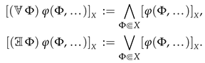


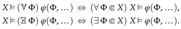


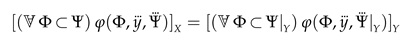
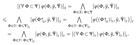
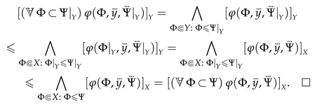


 by “reasoning inside X” (see Remark 11).
