Mechanical Models for Hermite Interpolation on the Unit Circle

Abstract

In the present paper, we delve into the study of nodal systems on the unit circle that meet certain separation properties. Our aim was to study the Hermite interpolation process on the unit circle by using these nodal arrays. The target was to develop the corresponding interpolation theory in order to make practical use of these nodal systems linked to certain mechanical models that fit these distributions.

1. Introduction

Hermite polynomial interpolation problems on the real line and on the bounded interval have been widely studied by many researchers. Most of the main contributions have been obtained by using as nodal points the zeros of the classical orthogonal polynomials and some of their generalizations (see [1,2,3]). When the nodal points are zeros of general orthogonal polynomials, the papers of Freud [4,5] (see [6]) deserve to be mentioned. The first attempt to use nodal systems not linked to measures and therefore to orthogonal polynomials was carried out by Fejér who introduced the so-called normal systems. In the same direction, we must mention the contributions of Grünwald who introduced in [7] the strongly normal nodal systems. Unfortunately, the use of these systems has not been consolidated and has not been continued. More recently, some nodal systems called well-spaced ones have been used for studying Lagrange interpolation problems. Although they are not connected with measures, any reasonable choice of interpolation nodes fulfills the conditions of being well spaced (see [8]). Thus, if one wants to work on the bounded interval with nodal systems that are not connected with measures, it seems convenient that the nodes have a distribution that is not far from the Chebyshev distribution. This closeness can be established in terms of suitable separation properties. The advantages of using these types of nodal systems is that they can be obtained through a random uniform distribution (see the examples given in [9]).

During the last few decades, several problems related to Hermite polynomial interpolation on the unit circle have been studied in depth. In some cases, the study has been connected to the Hermite interpolation on the interval and to the trigonometric interpolation. The nodal systems usually employed were the equispaced ones, that is those constituted by the n roots of complex numbers with modulus one. It is well known that there are methods to compute the Laurent polynomials of Hermite interpolation in an efficient way, when considering equally spaced nodal points on the unit circumference. By using these nodal systems, the convergence of the Hermite–Fejér interpolation polynomials related to continuous functions was studied in [10], obtaining a Fejér-type theorem. The convergence of the Hermite interpolation polynomials taking nonvanishing conditions for the derivatives was studied in [11] giving several versions of the second Fejér-type theorem.

Other more general nodal systems that have been used are those formed by the zeros of para-orthogonal polynomials, associated with good measures on the unit circle. We recall that a polynomial $Q_n\left(z\right)$ of degree n is para-orthogonal if it satisfies that $Q_n\left(z\right)=z^n\overline{Q_n}(1/z)$ and it is orthogonal to ${\left\{z^k\right\}}_{k=1}^{n-1}$ with respect to a measure on the unit circle. It deserves to mention measures in the Baxter class or analytic measures and, in particular, measures in the Szegő class with the Szegő function having an analytic extension outside the unit disk (see [12,13]). In these cases, the nodal points are characterized by satisfying suitable separation properties, and it is possible to obtain the properties of the nodal polynomials without the need to compute their zeros explicitly. Most of these properties play an important role in the results for convergence and related problems that were studied.

The use of another type of nodal system adds complexity to the problem due mainly to the difficulty of computing their zeros. In this sense, some advances have been made by using nodal polynomials that are close to the equispaced ones in the unit circumference and that can be obtained through a perturbation of the uniform random distribution. The starting point is to ask the nodes for some separation properties that allow obtaining the main properties of the nodal polynomials playing a fundamental role in the interpolation processes.

If the arguments of the nodal points are ${\theta }_j,j=1,\cdots ,n$, we recall that in the Baxter class, the separation property satisfied by the nodal points is ${\theta }_{j+1}-{\theta }_j=\frac{2\pi }{n}+\mathcal{O}\left(\frac{1}{n}\right)$ (see [14]). When the nodal points are the zeros of para-orthogonal polynomials with respect to analytic weights on the unit circle or with respect to measures in the Szegő class having an analytic extension outside the unit disk, then the separation property is ${\theta }_{j+1}-{\theta }_j=\frac{2\pi }{n}+\mathcal{O}\left(\frac{1}{n^2}\right)$ (see [15]). Thus, the nodal points behave like perturbations of the roots of complex unimodular numbers.

In [9], we changed the focus of the interpolation problem, and our starting point was to use nodal systems that were not related to measures and that were only characterized to fulfil certain separation properties between the nodes. Thus, we studied the Lagrange interpolation problem on the unit circle by using nodal systems that are not connected with any measure, and they are only characterized by satisfying a separation property of the type: ${\theta }_{j+1}-{\theta }_j=\frac{2\pi }{n}+\mathcal{O}\left(\frac{1}{n^2}\right).$ In the aforementioned paper, a detailed study of their properties was done. Moreover, the Lebesgue constant of the process was obtained, as well as some results for the convergence and the rate of convergence for different smooth continuous functions.

In the present paper, we studied nodal systems like those used in [9] that meet the separation properties mentioned above, and we present mechanical models that fit these distributions. The aim of this work was to study the Hermite interpolation process on the unit circle by using these nodal systems characterized by a separation property between the nodes. The target was to develop the corresponding interpolation theory that allows us to make practical use of these nodal systems linked to certain mechanical models. Thus, in the first part of the paper (see Section 2 and Section 3), we recall the properties given in [9] satisfied by the nodal system, and we obtain some new ones that play an important role in the Hermite process. Our main result was to prove a new version of Fejér’s theorem for continuous functions on the unit circle by using these nodal systems. We also studied the complete problem, that is the Hermite interpolation problem with nonvanishing conditions for the derivatives, giving a sufficient condition on the derivatives in order to assure convergence. These results are gathered in Section 4, with the study of the convergence of the Hermite interpolation polynomial related to analytic and smooth functions (see [16]), and finally, in Section 5 we obtain the corresponding results on the bounded interval. Indeed, we transformed the problem into a new one on the bounded interval studying the Hermite interpolation problem related to continuous functions on $[-1,1]$ and by using nodal points characterized by some separation properties. In Section 6, we present some mechanical models generating the nodal systems according to our distribution, as well as some numerical examples by applying our results. Finally, Section 7 gathers the main notation concerning the different classes of polynomials used throughout the paper; Section 8 briefs the materials and methods used and Section 9 offers a discussion of the problem.

2. Preliminaries

The aim of this paper was to study Hermite interpolation problems on the unit circle $\mathbb{T}=\{z\in \mathbb{C}:|z|=1\}$ by using nodal systems satisfying some suitable separation properties, which are not connected with orthogonality nor para-orthogonality with respect to any measure.

We denote the nodal polynomials by $W_n\left(z\right)$ and their zeros by ${\left\{{\alpha }_{j,n}\right\}}_{j=1}^n$, that is, we assumed that $W_n\left(z\right)={\Pi }_{j=1}^n(z-{\alpha }_{j,n})$, where $|{\alpha }_{j,n}|=1$ for $j=1,\cdots ,n$, and ${\alpha }_{j,n}\ne {\alpha }_{k,n}$ for $j\ne k.$ For simplicity, we omit the subscript n and write ${\alpha }_j$ instead of ${\alpha }_{j,n}$ for $j=1,\cdots ,n.$ First, we recall some well-known definitions related to interpolation problems on the unit circle. We work in the space of Laurent polynomials and, in particular, in the subspaces ${\Lambda }_{p,q}\left[z\right]=span\{z^k:p\le k\le q\}$, with p and q integers $p\le q$.

If ${\left\{u_j\right\}}_{j=1}^n$ and ${\left\{v_j\right\}}_{j=1}^n$ are arbitrary complex numbers and $W_n\left(z\right)$ is the nodal polynomial, then the Hermite interpolation problem consists of determining the Laurent polynomial ${\mathcal{H}}_{-n,n-1}\left(z\right)$ satisfying the interpolation conditions:

$${\mathcal{H}}_{-n,n-1}\left({\alpha }_j\right)=u_j,{\mathcal{H}}_{-n,n-1}^{\prime }\left({\alpha }_j\right)=v_j,\mathrm{for}j=1,\cdots ,n.$$

This polynomial can be rewritten as ${\mathcal{H}}_{-n,n-1}\left(z\right)={\mathcal{HF}}_{-n,n-1}\left(z\right)+{\mathcal{HD}}_{-n,n-1}\left(z\right),$ where the Hermite–Fejér interpolation polynomial satisfies that:

$${\mathcal{HF}}_{-n,n-1}\left({\alpha }_j\right)=u_j,{\mathcal{HF}}_{-n,n-1}^{\prime }\left({\alpha }_j\right)=0,\mathrm{for}j=1,\cdots ,n,$$

(1)

and ${\mathcal{HD}}_{-n,n-1}\left(z\right)$ satisfies that

$${\mathcal{HD}}_{-n,n-1}\left({\alpha }_j\right)=0,{\mathcal{HD}}_{-n,n-1}^{\prime }\left({\alpha }_j\right)=v_j,\mathrm{for}j=1,\cdots ,n.$$

(2)

If f is a function, $u_j=f\left({\alpha }_j\right)$ and $v_j=0$, we denote the corresponding Laurent polynomial ${\mathcal{HF}}_{-n,n-1}(f,z)$. In the same way, if $u_j=0,v_j=f^{\prime }\left({\alpha }_j\right)$, we denote the corresponding Laurent polynomial by ${\mathcal{HD}}_{-n,n-1}(f,z)$ and also denote by ${\mathcal{H}}_{-n,n-1}(f,z)={\mathcal{HF}}_{-n,n-1}(f,z)+{\mathcal{HD}}_{-n,n-1}(f,z)$. In the case, when $u_j=f\left({\alpha }_j\right)$ and $v_j$ is arbitrary, if ${\gamma }_n={\left(v_j\right)}_{j=1}^n$, we denote by ${\mathcal{H}}_{-n,n-1}(f,{\gamma }_n,z)={\mathcal{HF}}_{-n,n-1}(f,z)+{\mathcal{HD}}_{-n,n-1}\left(z\right)$.

Let us recall that the preceding polynomials can be computed by using the following expressions (see [17]).

$${\mathcal{HF}}_{-n,n-1}\left(z\right)={\displaystyle \sum _{k=1}^n}{\mathfrak{h}}_{k,n}\left(z\right)u_k$$

(3)

and

$${\mathcal{HD}}_{-n,n-1}\left(z\right)={\displaystyle \sum _{k=1}^n}{\mathfrak{k}}_{k,n}\left(z\right)v_k,$$

(4)

where ${\mathfrak{h}}_{k,n}$ and ${\mathfrak{k}}_{k,n}$ are the fundamental polynomials of Hermite interpolation given by:

$${\mathfrak{h}}_{k,n}\left(z\right)=\frac{{\left(W_n\left(z\right)\right)}^2}{z^n}\frac{1}{{\left(W_n^{\prime }\left({\alpha }_k\right)\right)}^2}\left[\frac{{\alpha }_k^n}{{(z-{\alpha }_k)}^2}+\frac{{\alpha }_k^{n-1}}{(z-{\alpha }_k)}\left(n-\frac{{\alpha }_k{W}_n^{″}\left({\alpha }_k\right)}{W_n^{\prime }\left({\alpha }_k\right)}\right)\right],$$

(5)

and:

$${\mathfrak{k}}_{k,n}\left(z\right)=\frac{{\left(W_n\left(z\right)\right)}^2}{z^n}\frac{{\alpha }_k^n}{{\left(W_n^{\prime }\left({\alpha }_k\right)\right)}^2}\frac{1}{(z-{\alpha }_k)}.$$

(6)

We can obtain more suitable expressions of these polynomials by using the following relations:

If $z,{\alpha }_k\in \mathbb{T}$, then ${(z-{\alpha }_k)}^2=-z{\alpha }_k{|z-{\alpha }_k|}^2$, and therefore, if $W_n\left(z\right)={\displaystyle \prod _{k=1}^n}(z-{\alpha }_k)$, then we get ${\left(W_n\left(z\right)\right)}^2={(-1)}^n{z}^n\left({\displaystyle \prod _{k=1}^n}{\alpha }_k\right){\left|W_n\left(z\right)\right|}^2.$ Moreover, since $W_n^{\prime }\left({\alpha }_k\right)={\displaystyle \prod _{j=1,j\ne k}^n}({\alpha }_k-{\alpha }_j)$, then ${\left(W_n^{\prime }\left({\alpha }_k\right)\right)}^2={(-1)}^{n-1}{\alpha }_k^{n-2}\left({\displaystyle \prod _{j=1}^n}{\alpha }_j\right){\left|W_n^{\prime }\left({\alpha }_k\right)\right|}^2$.

Hence, by substituting these relations in (5) and (6), we obtain:

$${\mathfrak{h}}_{k,n}\left(z\right)=\frac{|W_n{\left(z\right)|}^2}{|W_n^{\prime }\left({\alpha }_k\right){|}^2}\left[\frac{{\alpha }_k}{z|z-{\alpha }_k{|}^2}-\frac{{\alpha }_k}{(z-{\alpha }_k)}\left(n-\frac{{\alpha }_k{W}_n^{″}\left({\alpha }_k\right)}{W_n^{\prime }\left({\alpha }_k\right)}\right)\right],$$

(7)

and:

$${\mathfrak{k}}_{k,n}\left(z\right)=-\frac{|W_n{\left(z\right)|}^2}{|W_n^{\prime }\left({\alpha }_k\right){|}^2}\frac{{\alpha }_k^2}{(z-{\alpha }_k)},$$

(8)

and therefore, we have the following desired expressions for the Hermite interpolation polynomials:

$${\mathcal{HF}}_{-n,n-1}\left(z\right)={\displaystyle \sum _{k=1}^n}\frac{|W_n{\left(z\right)|}^2}{|W_n^{\prime }\left({\alpha }_k\right){|}^2}\left[\frac{{\alpha }_k}{z|z-{\alpha }_k{|}^2}-\frac{{\alpha }_k}{(z-{\alpha }_k)}\left(n-\frac{{\alpha }_k{W}_n^{″}\left({\alpha }_k\right)}{W_n^{\prime }\left({\alpha }_k\right)}\right)\right]u_k,$$

(9)

and

$${\mathcal{HD}}_{-n,n-1}\left(z\right)=-{\displaystyle \sum _{k=1}^n}\frac{|W_n{\left(z\right)|}^2}{|W_n^{\prime }\left({\alpha }_k\right){|}^2}\frac{{\alpha }_k^2}{(z-{\alpha }_k)}{v}_k.$$

(10)

In practice, it is more convenient to use the barycentric expressions for computing the interpolation polynomials. Thus, in what follows, we obtain these types of formulas.

By taking into account that ${\mathcal{H}}_{-n,n-1}\left(z\right)={\mathcal{HF}}_{-n,n-1}\left(z\right)+{\mathcal{HD}}_{-n,n-1}\left(z\right)$ and $1={\mathcal{HF}}_{-n,n-1}(1,z),$ then we get:

$${\mathcal{H}}_{-n,n-1}\left(z\right)=\frac{\mathcal{H}{\mathcal{F}}_{-n,n-1}\left(z\right)+\mathcal{H}{\mathcal{D}}_{-n,n-1}\left(z\right)}{\mathcal{H}{\mathcal{F}}_{-n,n-1}(1,z)}.$$

Thus, if we use (3) and (4), we have:

$${\displaystyle {\mathcal{H}}_{-n,n-1}\left(z\right)=\frac{{\displaystyle {\displaystyle \sum _{k=1}^n}{\mathfrak{h}}_{k,n}\left(z\right)u_k+{\displaystyle \sum _{k=1}^n}{\mathfrak{k}}_{k,n}\left(z\right)v_k}}{{\displaystyle {\displaystyle \sum _{k=1}^n}{\mathfrak{h}}_{k,n}\left(z\right)}}.}$$

On the one hand, if we apply (5) and (6), we obtain the following barycentric expression:

$${\displaystyle {\mathcal{H}}_{-n,n-1}\left(z\right)=\frac{{\displaystyle {\displaystyle \sum _{k=1}^n}\frac{{\alpha }_k^{n-1}}{{\left(W_n^{\prime }\left({\alpha }_k\right)\right)}^2}\left[\left[\frac{{\alpha }_k}{{(z-{\alpha }_k)}^2}+\frac{1}{(z-{\alpha }_k)}\left(n-\frac{{\alpha }_k{W}_n^{″}\left({\alpha }_k\right)}{W_n^{\prime }\left({\alpha }_k\right)}\right)\right]u_k+\frac{{\alpha }_k}{(z-{\alpha }_k)}{v}_k\right]}}{{\displaystyle {\displaystyle \sum _{k=1}^n}\frac{{\alpha }_k^{n-1}}{{\left(W_n^{\prime }\left({\alpha }_k\right)\right)}^2}\left[\frac{{\alpha }_k}{{(z-{\alpha }_k)}^2}+\frac{1}{(z-{\alpha }_k)}\left(n-\frac{{\alpha }_k{W}_n^{″}\left({\alpha }_k\right)}{W_n^{\prime }\left({\alpha }_k\right)}\right)\right]}}.}$$

On the other hand, if we use Equations (7) and (8) instead of (5) and (6), we obtain the equivalent barycentric expression:

$${\displaystyle {\mathcal{H}}_{-n,n-1}\left(z\right)=\frac{{\displaystyle {\displaystyle \sum _{k=1}^n}\frac{1}{|W_n^{\prime }\left({\alpha }_k\right){|}^2}\left[\left[\frac{{\alpha }_k}{z|z-{\alpha }_k{|}^2}-\frac{{\alpha }_k}{(z-{\alpha }_k)}\left(n-\frac{{\alpha }_k{W}_n^{″}\left({\alpha }_k\right)}{W_n^{\prime }\left({\alpha }_k\right)}\right)\right]u_k-\frac{{\alpha }_k^2}{(z-{\alpha }_k)}{v}_k\right]}}{{\displaystyle {\displaystyle \sum _{k=1}^n}\frac{1}{|W_n^{\prime }\left({\alpha }_k\right){|}^2}\left[\frac{{\alpha }_k}{z|z-{\alpha }_k{|}^2}-\frac{{\alpha }_k}{(z-{\alpha }_k)}\left(n-\frac{{\alpha }_k{W}_n^{″}\left({\alpha }_k\right)}{W_n^{\prime }\left({\alpha }_k\right)}\right)\right]}}.}$$

(11)

Proceeding in a similar way, we can obtain the two following barycentric expressions for the Hermite–Fejér interpolation polynomial:

$${\displaystyle {\mathcal{HF}}_{-n,n-1}\left(z\right)=\frac{{\displaystyle {\displaystyle \sum _{k=1}^n}\frac{{\alpha }_k^{n-1}}{{\left(W_n^{\prime }\left({\alpha }_k\right)\right)}^2}\left[\frac{{\alpha }_k}{{(z-{\alpha }_k)}^2}+\frac{1}{(z-{\alpha }_k)}\left(n-\frac{{\alpha }_k{W}_n^{″}\left({\alpha }_k\right)}{W_n^{\prime }\left({\alpha }_k\right)}\right)\right]u_k}}{{\displaystyle {\displaystyle \sum _{k=1}^n}\frac{{\alpha }_k^{n-1}}{{\left(W_n^{\prime }\left({\alpha }_k\right)\right)}^2}\left[\frac{{\alpha }_k}{{(z-{\alpha }_k)}^2}+\frac{1}{(z-{\alpha }_k)}\left(n-\frac{{\alpha }_k{W}_n^{″}\left({\alpha }_k\right)}{W_n^{\prime }\left({\alpha }_k\right)}\right)\right]}},}$$

$${\displaystyle {\mathcal{HF}}_{-n,n-1}\left(z\right)=\frac{{\displaystyle {\displaystyle \sum _{k=1}^n}\frac{1}{|W_n^{\prime }\left({\alpha }_k\right){|}^2}\left[\frac{{\alpha }_k}{z|z-{\alpha }_k{|}^2}-\frac{{\alpha }_k}{(z-{\alpha }_k)}\left(n-\frac{{\alpha }_k{W}_n^{″}\left({\alpha }_k\right)}{W_n^{\prime }\left({\alpha }_k\right)}\right)\right]u_k}}{{\displaystyle {\displaystyle \sum _{k=1}^n}\frac{1}{|W_n^{\prime }\left({\alpha }_k\right){|}^2}\left[\frac{{\alpha }_k}{z|z-{\alpha }_k{|}^2}-\frac{{\alpha }_k}{(z-{\alpha }_k)}\left(n-\frac{{\alpha }_k{W}_n^{″}\left({\alpha }_k\right)}{W_n^{\prime }\left({\alpha }_k\right)}\right)\right]}}.}$$

(12)

3. The Focus: The Nodal System

Throughout the paper, we assume that the zeros of the nodal polynomials $W_n\left(z\right)$ satisfy the following separation property: there exists a positive constant A, $A<\pi$ such that the length of the shortest arc between two consecutive nodes ${\alpha }_j$ and ${\alpha }_{j+1}$ satisfies:

$$\widehat{{\alpha }_j-{\alpha }_{j+1}}=\frac{2\pi }{n}+\frac{A\left(j\right)}{n^2}\mathrm{with}\left|A\left(j\right)\right|\le A,\forall j=1,\cdots ,n,$$

(13)

where ${\alpha }_{n+1}={\alpha }_1$. As we said before, we denote the length of the shortest arc between any two points of the unit circle, $z_1$ and $z_2$, by $\widehat{z_1-z_2}.$

If we use Landau’s notation for complex sequences, denoting by $a_n=\mathcal{O}\left(b_n\right)$ if $|\frac{a_n}{b_n}|$ is bounded, then the preceding property can be formulated as follows:

$$\widehat{{\alpha }_j-{\alpha }_{j+1}}=\frac{2\pi }{n}+\mathcal{O}\left(\frac{1}{n^2}\right).$$

We use the same $\mathcal{O}$ to denote different sequences. Unless we mention it explicitly, the limits we obtained from (13) were uniform.

We also considered other nodal polynomials, ${\tilde{W}}_{n,j}\left(z\right),j=1,\cdots ,n$, well connected with $W_n\left(z\right)$. We define ${\tilde{W}}_{n,j}\left(z\right)=z^n-{\lambda }_j$, with ${\lambda }_j={\alpha }_j^n$, and we denote their zeros by ${\beta }_{k,j}=\sqrt[n]{{\lambda }_j},k=1,\cdots ,n,\mathrm{and\; it\; holds}{\beta }_{1,j}={\alpha }_j.$

In what follows, we take for simplicity $j=1$, that is we work with ${\tilde{W}}_{n,1}\left(z\right)=z^n-{\lambda }_1$, and in order to simplify the notation, we denote ${\tilde{W}}_{n,1}\left(z\right)$ by ${\tilde{W}}_n\left(z\right)$ and its zeros ${\beta }_{k,1}$ by ${\beta }_k$ for $k=1,\cdots ,n$, with ${\beta }_{1,1}={\beta }_1={\alpha }_1$.

Hence, it is clear that the separation property satisfied by the zeros $\left\{{\beta }_j\right\}$ of ${\tilde{W}}_n\left(z\right)$ is:

$$\widehat{{\beta }_j-{\beta }_{j+1}}=\frac{2\pi }{n},\forall j=1,\cdots ,n,$$

(14)

where ${\beta }_{n+1}={\beta }_1$.

In this section, we present the properties satisfied by these nodal polynomials $W_n\left(z\right)$ that play an important role in our interpolatory scheme.

First, we recall the following well-known relation between arcs and strings that we use to obtain the nodal properties based on the convex character of the arcsin function:

If $z_1$ and $z_2$ belong to $\mathbb{T}$, then:

$$\frac{2}{\pi }\left(\widehat{z_1-z_2}\right)\le |z_1-z_2|\le \left(\widehat{z_1-z_2}\right).$$

(15)

Secondly, we recall a separation property, given in [9], between both nodal systems $W_n\left(z\right)$ and ${\tilde{W}}_n\left(z\right)$.

If ${\left\{{\alpha }_j\right\}}_{j=1}^n$ and ${\left\{{\beta }_j\right\}}_{j=1}^n$, with ${\alpha }_1={\beta }_1$, are the nodal points satisfying the separation properties (13) and (14), respectively, and we assume they are numbered in the clockwise sense, then:

$$\widehat{{\alpha }_j-{\beta }_j}\le (j-1)\frac{A}{n^2},\mathrm{for} j\ge 1,\mathrm{and} \widehat{{\alpha }_{n-j}-{\beta }_{n-j}}\le (j+1)\frac{A}{n^2}, \mathrm{for} j\ge 0.$$

Notice that we can write the preceding relations as follows:

$$\widehat{{\alpha }_j-{\beta }_j}=(j-1)\mathcal{O}\left(\frac{1}{n^2}\right),\mathrm{for} j\ge 1,\mathrm{and} \widehat{{\alpha }_{n-j}-{\beta }_{n-j}}=(j+1)\mathcal{O}\left(\frac{1}{n^2}\right),\mathrm{for} j\ge 0.$$

(16)

In the next propositions, we present the main properties of the nodal polynomials $W_n\left(z\right)$ involved in the interpolatory schemes of Lagrange and Hermite.

Proposition 1.

(i) 

For every n, it holds:

$$|W_n\left(z\right)|<2e^A and \frac{|W_n^{\prime }\left(z\right)|}{n}<2e^A,\forall z\in \mathbb{T}.$$

(17)

(ii) 

There exists a positive constant $C>0$ such that for n large enough:

$$\frac{|W_n^{\prime }\left({\alpha }_j\right)|}{n}>C,\forall j=1,\cdots ,n.$$

(18)

(iii) 

There exists a positive constant $D>0$ such that for every n:

$$\frac{|W_n{\left(z\right)|}^2}{n^2}{\displaystyle \sum _{j=1}^n}\frac{1}{|z-{\alpha }_j{|}^2}<D,\forall z\in \mathbb{T}.$$

(19)

Proof. 

See [9]. □

We finish the section with the next property, which turns out to be the key property to study the convergence of the Hermite interpolation polynomials.

Proposition 2.

There exists a positive constant $E>0$ such that for every n:

$$|n{W}_n^{\prime }\left({\alpha }_j\right)-{\alpha }_j{W}_n^{″}\left({\alpha }_j\right)|<Enlogn,{\forall }_j=1,\cdots ,n.$$

(20)

Proof. 

Since $|n{W}_n^{\prime }\left({\alpha }_j\right)-{\alpha }_j{W}_n^{″}\left({\alpha }_j\right)|=|W_n^{\prime }\left({\alpha }_j\right)\left|\right|n-\frac{{\alpha }_j{W}_n^{″}\left({\alpha }_j\right)}{W_n^{\prime }\left({\alpha }_j\right)}|$, by applying (17), we obtain that $|n{W}_n^{\prime }\left({\alpha }_j\right)-{\alpha }_j{W}_n^{″}\left({\alpha }_j\right)|\le 2n{e}^A|n-\frac{{\alpha }_j{W}_n^{″}\left({\alpha }_j\right)}{W_n^{\prime }\left({\alpha }_j\right)}|$.

Thus, we prove that there exists a positive constant F such that:

$$|n-\frac{{\alpha }_j{W}_n^{″}\left({\alpha }_j\right)}{W_n^{\prime }\left({\alpha }_j\right)}|\le Flogn,$$

and for simplicity and without loss of generality, we took, in what follows, $j=1$. If we write $W_n\left(z\right)=(z-{\alpha }_1)P_{n-1}\left(z\right)$, with ${\displaystyle P_{n-1}\left(z\right)={\displaystyle \prod _{j=2}^n}(z-{\alpha }_j)}$, then ${\displaystyle W_n^{\prime }\left({\alpha }_1\right)=P_{n-1}\left({\alpha }_1\right)={\displaystyle \prod _{j=2}^n}({\alpha }_1-{\alpha }_j)}$ and ${\displaystyle W_n^{″}\left({\alpha }_1\right)=2P_{n-1}^{\prime }\left({\alpha }_1\right)={\displaystyle \sum _{k=2}^n}{\displaystyle \prod _{j=2,j\ne k}^n}({\alpha }_1-{\alpha }_j).}$ Hence:

$$\frac{{\alpha }_1{W}_n^{″}\left({\alpha }_1\right)}{W_n^{\prime }\left({\alpha }_1\right)}=\frac{2{\alpha }_1{P}_{n-1}^{\prime }\left({\alpha }_1\right)}{P_{n-1}\left({\alpha }_1\right)}=2{\displaystyle \sum _{j=2}^n}\frac{1}{1-\left(\frac{{\alpha }_j}{{\alpha }_1}\right)}.$$

(21)

Since ${\alpha }_j={\beta }_j{e}^{i\widehat{({\beta }_j-{\alpha }_j)}}$, then ${\displaystyle \frac{{\alpha }_j}{{\alpha }_1}=\frac{{\beta }_j}{{\beta }_1}{e}^{i\widehat{({\beta }_j-{\alpha }_j)}}={\delta }_j{e}^{i\widehat{({\beta }_j-{\alpha }_j)}},j=2,\cdots ,n}$, where ${\left\{{\delta }_j\right\}}_{j=2}^n$ are the n-th roots of the unity different from one. By taking into account (16), we have that:

$$1-\frac{{\alpha }_j}{{\alpha }_1}=1-{\delta }_j{e}^{i(j-1)\mathcal{O}\left(\frac{1}{n^2}\right)}=1-{\delta }_j-(j-1)\mathcal{O}\left(\frac{1}{n^2}\right),$$

where $\mathcal{O}\left(\frac{1}{n^2}\right)=\frac{A_n}{n^2}$, with $|A_n|\le A$. Hence, (21) can be rewritten as:

$$\frac{{\alpha }_1{W}_n^{″}\left({\alpha }_1\right)}{W_n^{\prime }\left({\alpha }_1\right)}=2{\displaystyle \sum _{j=2}^n}\frac{1}{1-{\delta }_j-(j-1)\mathcal{O}\left(\frac{1}{n^2}\right)}.$$

(22)

In order to simplify the calculus in the preceding sum, we used the identity:

$$\frac{\mathcal{A}}{\mathcal{B}+\mathcal{D}}=\frac{\mathcal{A}}{\mathcal{B}}-\frac{\mathcal{A}\mathcal{D}}{\mathcal{B}(\mathcal{B}+\mathcal{D})}$$

(23)

taking $\mathcal{A}=1$, $\mathcal{B}=1-{\delta }_j$, and $\mathcal{D}=-(j-1)\mathcal{O}\left(\frac{1}{n^2}\right)$. To analyze $\mathcal{B}=1-{\delta }_j$, we took into account that:

$$\frac{2}{\pi }\widehat{(1-{\delta }_j)}\le |1-{\delta }_j|\le \widehat{(1-{\delta }_j)},$$

that is,

$$\frac{4}{n}(j-1)\le |1-{\delta }_j|\le \frac{2\pi }{n}(j-1).$$

Hence, $1-{\delta }_j=(j-1){\mathcal{O}}_1\left(\frac{1}{n}\right)$, where ${\mathcal{O}}_1\left(\frac{1}{n}\right)=\frac{B_n}{n}$, with $4<|B_n|<2\pi$. Now, by applying (23) in Equation (22), we can rewrite (21) as follows:

$$\begin{array}{c}\hfill \frac{{\alpha }_1{W}_n^{″}\left({\alpha }_1\right)}{W_n^{\prime }\left({\alpha }_1\right)}=2{\displaystyle \sum _{j=2}^n}\left(\frac{1}{1-{\delta }_j}+\frac{(j-1)\mathcal{O}\left(\frac{1}{n^2}\right)}{(j-1){\mathcal{O}}_1\left(\frac{1}{n}\right)[(j-1){\mathcal{O}}_1\left(\frac{1}{n}\right)-(j-1)\mathcal{O}\left(\frac{1}{n^2}\right)]}\right)\end{array}$$

Hence, if we use that $2{\sum }_{j=2}^n\frac{1}{1-{\delta }_j}=n-1$, then:

$$\frac{{\alpha }_1{W}_n^{″}\left({\alpha }_1\right)}{W_n^{\prime }\left({\alpha }_1\right)}-n=-1+2{\displaystyle \sum _{j=2}^n}\frac{\mathcal{O}\left(\frac{1}{n^2}\right)}{(j-1){\mathcal{O}}_1\left(\frac{1}{n}\right)[{\mathcal{O}}_1\left(\frac{1}{n}\right)-\mathcal{O}\left(\frac{1}{n^2}\right)]}$$

and therefore:

$$\begin{array}{c}\hfill \left|\frac{{\alpha }_1{W}_n^{″}\left({\alpha }_1\right)}{W_n^{\prime }\left({\alpha }_1\right)}-n\right|=\left|-1+2{\displaystyle \sum _{j=2}^n}\frac{\frac{A_n}{n^2}}{(j-1)\frac{B_n}{n}(\frac{B_n}{n}-\frac{A_n}{n^2})}\right|\le 1+2{\displaystyle \sum _{j=2}^n}\frac{|A_n|}{(j-1)|B_n(B_n-\frac{A_n}{n})|}<\\ \hfill 1+\frac{A}{2}{\displaystyle \sum _{j=2}^n}\frac{1}{(j-1)|B_n-\frac{A_n}{n}|}.\end{array}$$

Since $|B_n-\frac{A_n}{n}|\ge |B_n|-\frac{|A_n|}{n}>4-\frac{A}{n}>4-\pi$, then:

$$\left|\frac{{\alpha }_1{W}_n^{″}\left({\alpha }_1\right)}{W_n^{\prime }\left({\alpha }_1\right)}-n\right|<1+\frac{A}{2(4-\pi )}{\displaystyle \sum _{j=2}^n}\frac{1}{j-1}=1+\frac{A}{2(4-\pi )}(log(n-1)+\mathcal{C}+{\epsilon }_{n-1}),$$

with ${\epsilon }_{n-1}=o\left(1\right)$. Therefore, it is immediate that the last expression is $\mathcal{O}(logn)$, and thus, the proposition is proven. Notice that for another nodal point ${\alpha }_j$ with $j\ne 1$, one can proceed in a similar way. □

Remark 1.

In [17], we considered as nodal polynomials the para-orthogonal polynomials related to measures in the Szegő class with the Szegő function having an analytic extension outside the unit disk (see [12,13]). In this situation, Condition (13) is satisfied (see [15]) and Properties (17), (18), and (19) also hold, but Property (20) was different. Now, in the present paper, we had that $|n{W}_n^{\prime }\left({\alpha }_j\right)-{\alpha }_j{W}_n^{″}\left({\alpha }_j\right)|<Enlogn$, while in [17], the relation was $|n{W}_n^{\prime }\left({\alpha }_j\right)-{\alpha }_j{W}_n^{″}\left({\alpha }_j\right)|<En$.

4. Hermite–Fejér and Hermite Processes

4.1. Convergence of Hermite–Fejér Interpolation in the Case of Continuous Functions

Next, by following the ideas given in [10] for extending Fejér’s theorem for continuous functions (see [18]) to the unit circle, we obtained our main result. Reference [10] was the first extension in the case when the nodal points are the n roots of a complex number unimodular. In [17], Fejér’s theorem was proven when the nodal polynomial was para-orthogonal with respect to appropriate measures or when it satisfied certain properties. Now, we give a new version of Fejér’s theorem for continuous functions on the unit circle with nodal systems satisfying (13).

Theorem 1.

If F is a continuous function on $\mathbb{T}$, then ${\mathcal{HF}}_{-n,n-1}(F,z)$ converges to F uniformly on $\mathbb{T}$.

Proof. 

Since ${\mathcal{HF}}_{-n,n-1}(F,z)={\sum }_{k=1}^n{\mathfrak{h}}_{k,n}\left(z\right)F\left({\alpha }_k\right)$ and $F\left(z\right)=F\left(z\right){\sum }_{k=1}^n{\mathfrak{h}}_{k,n}\left(z\right)$, then we have:

$$|F\left(z\right)-{\mathcal{HF}}_{-n,n-1}(F,z)|\le {\displaystyle \sum _{k=1}^n}|{\mathfrak{h}}_{k,n}\left(z\right)||F\left(z\right)-F\left({\alpha }_k\right)|.$$

(24)

By taking into account that for $\epsilon >0$, there exists $\delta >0$ such that if $|z-y|<\delta$, then $|F(z)-F(y)|<\epsilon$, let us take n such that $\frac{1}{\sqrt[4]{n}}<\delta$.

Thus, we rewrite the last term of (24) as follows:

$${\displaystyle \sum _{k=1}^n}|{\mathfrak{h}}_{k,n}\left(z\right)||F\left(z\right)-F\left({\alpha }_k\right)|=\sum _{k\in I_{1,n}}|{\mathfrak{h}}_{k,n}\left(z\right)||F\left(z\right)-F\left({\alpha }_k\right)|+\sum _{k\in I_{2,n}}|{\mathfrak{h}}_{k,n}\left(z\right)||F\left(z\right)-F\left({\alpha }_k\right)|,$$

where $I_{1,n}=\{k\in \{1,\cdots ,n\}:|z-{\alpha }_k|<\frac{1}{\sqrt[4]{n}}\}$ and $I_{2,n}=\{k\in \{1,\cdots ,n\}:|z-{\alpha }_k|\ge \frac{1}{\sqrt[4]{n}}\}.$

On the one hand, ${\displaystyle \sum _{k\in I_{2,n}}|{\mathfrak{h}}_{k,n}\left(z\right)||F\left(z\right)-F\left({\alpha }_k\right){|\le 2\Vert F\Vert }_{\infty }\sum _{k\in I_{2,n}}|{\mathfrak{h}}_{k,n}\left(z\right)|}$, and by using (7), (18), (20), and (17), respectively, we get:

$$\begin{array}{c}\hfill \sum _{k\in I_{2,n}}|{\mathfrak{h}}_{k,n}\left(z\right)|\le \\ \hfill |W_n{\left(z\right)|}^2\sum _{k\in I_{2,n}}\frac{1}{|W_n^{\prime }\left({\alpha }_k\right){|}^2{|z-{\alpha }_k|}^2}+{|W_n\left(z\right)|}^2\sum _{k\in I_{2,n}}\frac{1}{|z-{\alpha }_k|}\frac{|n{W}_n^{\prime }\left({\alpha }_k\right)-{\alpha }_k{W}_n^{″}\left({\alpha }_k\right)|}{|W_n^{\prime }\left({\alpha }_k\right){|}^3}\le \\ \hfill |W_n{\left(z\right)|}^2\sum _{k\in I_{2,n}}\frac{1}{n^2{C}^2}\frac{1}{|z-{\alpha }_k{|}^2}+{|W_n\left(z\right)|}^2\sum _{k\in I_{2,n}}\frac{1}{|z-{\alpha }_k|}\frac{Elogn}{n^2{C}^3}\le \\ \hfill 4e^{2A}\sum _{k\in I_{2,n}}\frac{1}{C^2{n}^{\frac{3}{2}}}+4e^{2A}\sum _{k\in I_{2,n}}\frac{Elogn}{C^3{n}^{\frac{7}{4}}}\le 4e^{2A}\left(\frac{1}{C^2{n}^{\frac{1}{2}}}+\frac{Elogn}{C^3{n}^{\frac{3}{4}}}\right),\end{array}$$

(25)

which goes to zero for n large enough. On the other hand, we also obtain ${\displaystyle \sum _{k\in I_{1,n}}|{\mathfrak{h}}_{k,n}\left(z\right)||F\left(z\right)-F\left({\alpha }_k\right)|\le \epsilon \sum _{k\in I_{1,n}}|{\mathfrak{h}}_{k,n}\left(z\right)|}$, and by applying (7), (18), (20), (17), and (19), respectively, we get:

$$\begin{array}{c}\hfill \sum _{k\in I_{1,n}}\left|{\mathfrak{h}}_{k,n}\left(z\right)\right|=\sum _{k\in I_{1,n}}\frac{|W_n{\left(z\right)|}^2}{|W_n^{\prime }\left({\alpha }_k\right){|}^2}\left|\frac{{\alpha }_k}{z|z-{\alpha }_k{|}^2}-\frac{{\alpha }_k}{(z-{\alpha }_k)}\left(n-\frac{{\alpha }_k{W}_n^{″}\left({\alpha }_k\right)}{W_n^{\prime }\left({\alpha }_k\right)}\right)\right|\le \\ \hfill \sum _{k\in I_{1,n}}\frac{|W_n{\left(z\right)|}^2}{|z-{\alpha }_k{|}^2}\left(\frac{1}{|W_n^{\prime }\left({\alpha }_k\right){|}^2}+\frac{|z-{\alpha }_k\left|\right|n{W}_n^{\prime }\left({\alpha }_k\right)-{\alpha }_k{W}_n^{″}\left({\alpha }_k\right)|}{|W_n^{\prime }\left({\alpha }_k\right){|}^3}\right)\le \\ \hfill \sum _{k\in I_{1,n}}\frac{|W_n{\left(z\right)|}^2}{|z-{\alpha }_k{|}^2}\left(\frac{1}{C^2{n}^2}+\frac{1}{\sqrt[4]{n}}\frac{Enlogn}{C^3{n}^3}\right)<D\left(\frac{1}{C^2}+\frac{Elogn}{C^3\sqrt[4]{n}}\right).\end{array}$$

(26)

Therefore, ${\displaystyle \sum _{k\in I_{1,n}}|{\mathfrak{h}}_{k,n}\left(z\right)\left|\right|F\left(z\right)-F\left({\alpha }_k\right)|\le \epsilon T,}$ for some positive constant T and n large enough. Hence the Hermite–Fejér-type theorem is proven. □

Corollary 1.

There exists a positive constant $L>0$ such that for every F bounded on $\mathbb{T}$, it holds that:

$$|{\mathcal{HF}}_{-n,n-1}{(F,z)|\le L\Vert F\Vert }_{\infty },$$

for every $z\in \mathbb{T}$.

Next, we studied the complete problem, that is the Hermite interpolation problem with nonvanishing conditions for the derivatives. In [17], under suitable conditions for the nodal systems, we gave a sufficient condition on the derivatives, which cannot be improved, in order to obtain convergence for continuous functions. Now, we prove that the same condition works.

Proposition 3.

Let F be a continuous function on $\mathbb{T}$, and assume that ${\gamma }_n=(v_1,\cdots ,v_n)$ satisfies that ${\displaystyle \underset{n\to \infty }{lim}\frac{\Vert {\gamma }_n{\Vert }_2}{n}=0,}$ then ${\mathcal{H}}_{-n,n-1}(F,{\gamma }_n,z)$ converges to F uniformly on $\mathbb{T}$.

Proof. 

If we apply Expression (10), we get:

$$\begin{array}{c}\hfill |{\mathcal{HD}}_{-n,n-1}\left(z\right)|=|{\displaystyle \sum _{k=1}^n}-\frac{|W_n{\left(z\right)|}^2}{|W_n^{\prime }\left({\alpha }_k\right){|}^2}\frac{{\alpha }_k^2}{(z-{\alpha }_k)}{v}_k|\le |W_n{\left(z\right)|}^2{\displaystyle \sum _{k=1}^n}\frac{1}{|W_n^{\prime }\left({\alpha }_k\right){|}^2}\frac{|v_k|}{|z-{\alpha }_k|}\le \\ \hfill \frac{|W_n{\left(z\right)|}^2}{C^2{n}^2}{\displaystyle \sum _{k=1}^n}\frac{|v_k|}{|z-{\alpha }_k|}\le \frac{|W_n{\left(z\right)|}^2}{C^2{n}^2}{\left({\displaystyle \sum _{k=1}^n}\frac{1}{|z-{\alpha }_k{|}^2}\right)}^{\frac{1}{2}}{\left({\displaystyle \sum _{k=1}^n}{|v_k|}^2\right)}^{\frac{1}{2}}\le \\ \hfill \le \frac{|W_n\left(z\right)|}{C^{2}n}{\left({\displaystyle \sum _{k=1}^n}\frac{|W_n{\left(z\right)|}^2}{n^2{|z-{\alpha }_k|}^2}\right)}^{\frac{1}{2}}\Vert {\gamma }_n{\Vert }_2<\frac{2e^A}{C^{2}n}\sqrt{D}{\Vert {\gamma }_n\Vert }_2,\end{array}$$

(27)

which goes to zero uniformly on $\mathbb{T}$. Hence, if we take into account ${\mathcal{H}}_{-n,n-1}(F,{\gamma }_n,z)={\mathcal{HF}}_{-n,n-1}(F,z)+{\mathcal{HD}}_{-n,n-1}\left(z\right)$ joint with Theorem 1, then the result is proven. □

Notice that following the ideas given in [11], it is possible to give other sufficient conditions.

4.2. Convergence of Hermite Interpolation in the Case of Smooth Functions

This section is devoted to studying the convergence of the Hermite interpolation polynomials related to analytic functions and certain types of smooth functions.

Proposition 4.

If F is an analytic function in an open annulus containing $\mathbb{T}$, then ${\mathcal{H}}_{-n,n-1}(F,z)$ uniformly converges to F on $\mathbb{T}$, and the order of convergence is geometric.

Proof. 

F can be written ${\displaystyle F\left(z\right)={\displaystyle \sum _{j=-\infty }^{\infty }}{A}_j{z}^j}$, with $|A_j|\le P{r}^{\left|j\right|}$ for some $P>0$ and $0<r<1$. Thus, if we decompose $F\left(z\right)=F_{1,n}\left(z\right)+F_{2,n}\left(z\right)+F_{3,n}\left(z\right)$, with ${\displaystyle F_{1,n}\left(z\right)={\displaystyle \sum _{j=-n}^{n-1}}{A}_j{z}^j}$, ${\displaystyle F_{2,n}\left(z\right)={\displaystyle \sum _{j=n}^{\infty }}{A}_j{z}^j}$, and ${\displaystyle F_{3,n}\left(z\right)={\displaystyle \sum _{j=-\infty }^{-n-1}}{A}_j{z}^j}$, then it is clear that ${\mathcal{H}}_{-n,n-1}(F_{1,n},z)=F_{1,n}\left(z\right)$. Now, to obtain our result, first we studied the behavior of the difference $|{\mathcal{H}}_{-n,n-1}(F_{2,n},z)-F_{2,n}\left(z\right)|.$ Indeed:

$$\begin{array}{c}\hfill |{\mathcal{H}}_{-n,n-1}(F_{2,n},z)-F_{2,n}\left(z\right)|=|{\displaystyle \sum _{j=n}^{\infty }}{A}_j{z}^j-{\displaystyle \sum _{j=n}^{\infty }}{A}_j{\mathcal{H}}_{-n,n-1}(z^j,z)|=\\ \hfill |{\displaystyle \sum _{j=n}^{\infty }}{A}_j{z}^j-{\displaystyle \sum _{j=n}^{\infty }}{A}_j{\displaystyle \sum _{k=1}^n}{\mathfrak{h}}_{k,n}\left(z\right){\alpha }_k^j-{\displaystyle \sum _{j=n}^{\infty }}{A}_j{\displaystyle \sum _{k=1}^n}{\mathfrak{k}}_{k,n}\left(z\right)j{\alpha }_k^{j-1}|=\\ \hfill |{\displaystyle \sum _{j=n}^{\infty }}{A}_j\left(z^j-{\displaystyle \sum _{k=1}^n}{\mathfrak{h}}_{k,n}\left(z\right){\alpha }_k^j-{\displaystyle \sum _{k=1}^n}{\mathfrak{k}}_{k,n}\left(z\right)j{\alpha }_k^{j-1}\right)|\le \\ \hfill {\displaystyle \sum _{j=n}^{\infty }}|A_j|\left(1+{\displaystyle \sum _{k=1}^n}|{\mathfrak{h}}_{k,n}\left(z\right)|+{\displaystyle \sum _{k=1}^n}j|{\mathfrak{k}}_{k,n}\left(z\right)|\right).\end{array}$$

By taking into account (25) and (26), we get that:

$${\displaystyle \sum _{k=1}^n}\left|{\mathfrak{h}}_{k,n}\left(z\right)\right|\le 4e^{2A}\left(\frac{1}{C^2{n}^{\frac{1}{2}}}+\frac{Elogn}{C^3{n}^{\frac{3}{4}}}\right)+D\left(\frac{1}{C^2}+\frac{Elogn}{C^3\sqrt[4]{n}}\right)\le M+Q\frac{logn}{\sqrt{n}},$$

(28)

for some positive constants M and Q.

In the same way, by using (6) and (27) with ${\gamma }_n=(1,\cdots ,1)$, we have:

$${\displaystyle \sum _{k=1}^n}|{\mathfrak{k}}_{k,n}\left(z\right)|=|W_n{\left(z\right)|}^2{\displaystyle \sum _{k=1}^n}\frac{1}{|W_n^{\prime }\left({\alpha }_k\right){|}^2}\frac{1}{|z-{\alpha }_k|}\le \frac{2e^A}{C^{2}n}\sqrt{D}\sqrt{n}\le \frac{R}{\sqrt{n}},$$

(29)

for some positive constant R.

Hence:

$$\begin{array}{c}\hfill |{\mathcal{H}}_{-n,n-1}(F_{2,n},z)-F_{2,n}\left(z\right)|\le \\ \hfill {\displaystyle \sum _{j=n}^{\infty }}\left|A_j\right|\left(1+M+Q\frac{logn}{\sqrt{n}}+j\frac{R}{\sqrt{n}}\right)\le {\displaystyle \sum _{j=n}^{\infty }}P{r}^j\left(1+M+Q\frac{logn}{\sqrt{n}}+j\frac{R}{\sqrt{n}}\right)\le \\ \hfill P\frac{r^n}{1-r}\left(1+M+Q\frac{logn}{\sqrt{n}}+\frac{\left(n(1-r)+r\right)}{(1-r)}\frac{R}{\sqrt{n}}\right)\le S{r}_1^n,\end{array}$$

for some positive constant $r_1$ such that $r<r_1<1$. Then, it is clear that it goes to zero uniformly on $\mathbb{T}$, and the order of convergence is geometric.

Finally, one can obtain an analogous result for the difference $|{\mathcal{H}}_{-n,n-1}(F_{3,n},z)-F_{3,n}\left(z\right)|$, and hence, the result is proven. □

Proposition 5.

If ${\displaystyle F\left(z\right)={\displaystyle \sum _{j=-\infty }^{\infty }}{A}_j{z}^j}$ is a function defined on $\mathbb{T}$ with $|A_j|\le K\frac{1}{{\left|j\right|}^c},$ for some positive constant $K,j\ne 0,c>2$, then ${\mathcal{H}}_{-n,n-1}(F,z)$ converges to $F\left(z\right)$ uniformly on $\mathbb{T}$. Moreover, the order of convergence is $\mathcal{O}\left(\frac{1}{{(n-1)}^{c-2}}\right)$.

Proof. 

If we decompose $F\left(z\right)=F_{1,n}\left(z\right)+F_{2,n}\left(z\right)+F_{3,n}\left(z\right)$, with ${\displaystyle F_{1,n}\left(z\right)={\displaystyle \sum _{j=-n}^{n-1}}{A}_j{z}^j}$, ${\displaystyle F_{2,n}\left(z\right)={\displaystyle \sum _{j=n}^{\infty }}{A}_j{z}^j}$, and ${\displaystyle F_{3,n}\left(z\right)={\displaystyle \sum _{j=-\infty }^{-n-1}}{A}_j{z}^j}$, then:

$${\mathcal{H}}_{-n,n-1}(F,z)={\mathcal{H}}_{-n,n-1}(F_{1,n},z)+{\mathcal{H}}_{-n,n-1}(F_{2,n},z)+{\mathcal{H}}_{-n,n-1}(F_{3,n},z).$$

Since ${\mathcal{H}}_{-n,n-1}(F_{1,n},z)=F_{1,n}\left(z\right)$, then:

$$|{\mathcal{H}}_{-n,n-1}(F,z)-F\left(z\right)|\le |{\mathcal{H}}_{-n,n-1}(F_{2,n},z)-F_{2,n}\left(z\right)|+|{\mathcal{H}}_{-n,n-1}(F_{3,n},z)-F_{3,n}\left(z\right)|,$$

and we have to study the behavior of the differences $|{\mathcal{H}}_{-n,n-1}(F_{i,n},z)-F_{i,n}\left(z\right)|,i=2,3,$ to obtain the uniform convergence of ${\mathcal{H}}_{-n,n-1}(F,z)$ to F.

Indeed, if $z\in \mathbb{T}$:

$$\begin{array}{c}\hfill {\displaystyle |{\mathcal{H}}_{-n,n-1}(F_{2,n},z)-F_{2,n}\left(z\right)|=|{\mathcal{H}}_{-n,n-1}({\displaystyle \sum _{j=n}^{\infty }}{A}_j{z}^j,z)-{\displaystyle \sum _{j=n}^{\infty }}{A}_j{z}^j|=}\\ \hfill |{\displaystyle \sum _{j=n}^{\infty }}{A}_j{\mathcal{H}}_{-n,n-1}(z^j,z)-{\displaystyle \sum _{j=n}^{\infty }}{A}_j{z}^j|=|{\displaystyle \sum _{j=n}^{\infty }}{A}_j(z^j-{\mathcal{H}}_{-n,n-1}(z^j,z))|=\\ \hfill |{\displaystyle \sum _{j=n}^{\infty }}{A}_j(z^j-{\displaystyle \sum _{k=1}^n}{\mathfrak{h}}_{k,n}\left(z\right){\alpha }_k^j-{\displaystyle \sum _{k=1}^n}{\mathfrak{k}}_{k,n}\left(z\right)j{\alpha }_k^{j-1})|\le {\displaystyle \sum _{j=n}^{\infty }}|A_j|(1+{\displaystyle \sum _{k=1}^n}|{\mathfrak{h}}_{k,n}\left(z\right)|+j{\displaystyle \sum _{k=1}^n}|{\mathfrak{k}}_{k,n}\left(z\right)|).\end{array}$$

If we apply (28) and (29) in the preceding proposition, we get

$$\begin{array}{c}\hfill |{\mathcal{H}}_{-n,n-1}(F_{2,n},z)-F_{2,n}\left(z\right)|\le {\displaystyle \sum _{j=n}^{\infty }}|A_j|(1+M+Q\frac{logn}{\sqrt{n}}+j\frac{R}{\sqrt{n}})\le \\ \hfill {\displaystyle \sum _{j=n}^{\infty }}|A_j|S+{\displaystyle \sum _{j=n}^{\infty }}j|A_j|\frac{R}{\sqrt{n}}\le SK{\displaystyle \sum _{j=n}^{\infty }}\frac{1}{j^c}+\frac{RK}{\sqrt{n}}{\displaystyle \sum _{j=n}^{\infty }}\frac{1}{j^{c-1}}=\\ \hfill SK(H\left(c\right)-H_{n-1,c})+\frac{RK}{\sqrt{n}}(H(c-1)-H_{n-1,c-1})\le \\ \hfill \frac{SK}{(c-1){(n-1)}^{c-1}}+\frac{RK}{\sqrt{n}(c-2){(n-1)}^{c-2}},\end{array}$$

for some positive constant S, with $H\left(c\right)$ being the sum of the harmonic series ${\sum }_{j=1}^{\infty }\frac{1}{j^c}$ and $H_{n-1,c}$ its $(n-1)$-partial sum.

Hence, $|{\mathcal{H}}_{-n,n-1}(F_{2,n},z)-F_{2,n}\left(z\right)|$ goes to zero, and the order of convergence is $\mathcal{O}\left(\frac{1}{{(n-1)}^{c-2}}\right)$. Notice that the same result is valid for $|{\mathcal{H}}_{-n,n-1}(F_{3,n},z)-F_{3,n}\left(z\right)|$, and hence, the result is proven. □

Remark 2.

Notice that for smooth functions, we obtained closed results to those given in [16] related to the Chebyshev process on the bounded interval. In particular, for the functions studied in the previous proposition, we obtained an accuracy of $\mathcal{O}\left(\frac{1}{{(n-1)}^{c-2}}\right)$, while the Chebyshev-related result was $\mathcal{O}\left(\frac{1}{{(n-1)}^{c-1}}\right)$, which is a better result. However, for analytic functions, we obtained a quite similar result.

5. The Case of the Bounded Interval

In this section, we consider nodal systems in the interval $[-1,1]$, which are closely connected with those considered on the unit circle in Section 3. Indeed let us consider the nodal array ${\left\{x_j\right\}}_{j=1}^n\subset [-1,1]$ numbered as follows $-1\le x_n<x_{n-1}<\cdots <x_2<x_1\le 1.$ We distinguished four cases depending on $x_1=1$ or $x_1\ne 1$ and $x_n=-1$ or $x_n\ne -1$. In all the cases, we assumed that there exists a positive constant $A<\pi$ such that one of the following separation properties holds:

(i)

$x_1=1,x_n=-1$, and $arccos{x}_{j+1}-arccos{x}_j=\frac{\pi }{n}+\frac{a\left(j\right)}{n^2}$, with $|a(j)|\le A,\forall j=1,\cdots ,n-1.$

(ii)

$x_1<1,x_n=-1,$$arccos{x}_{j+1}-arccos{x}_j=\frac{\pi }{n}+\frac{a\left(j\right)}{n^2}$, with $|a(j)|\le A,\forall j=1,\cdots ,n-1,$ and $2arccos{x}_1=\frac{\pi }{n}+\frac{a\left(0\right)}{n^2}$, with $|a(0)|\le A.$

(iii)

$x_1=1,x_n>-1$, $arccos{x}_{j+1}-arccos{x}_j=\frac{\pi }{n}+\frac{a\left(j\right)}{n^2}$, with $|a(j)|\le A,\forall j=1,\cdots ,n-1,$ and $2(\pi -arccos{x}_n)=\frac{\pi }{n}+\frac{a\left(n\right)}{n^2}$, with $|a(n)|\le A.$

(iv)

$x_1<1,x_n>-1$, $arccos{x}_{j+1}-arccos{x}_j=\frac{\pi }{n}+\frac{a\left(j\right)}{n^2}$, with $|a(j)|\le A,\forall j=1,\cdots ,n-1,$$2arccos{x}_1=\frac{\pi }{n}+\frac{a\left(0\right)}{n^2}$, with $|a(0)|\le A,$ and $2(\pi -arccos{x}_n)=\frac{\pi }{n}+\frac{a\left(n\right)}{n^2}$, with $|a(n)|\le A.$

Our aim was to study Hermite interpolation problems on the interval with these nodal systems. First, we considered a real function f continuous on $[-1,1]$, and we studied the convergence of the Hermite interpolation polynomial $h_{2n-1}(f,x)$ satisfying the conditions:

$$h_{2n-1}(f,x_j)=f\left(x_j\right),h_{2n-1}^{\prime }(f,x_j)=v_j,\mathrm{with}{v}_j\in \mathbb{R},j=1,\cdots ,n.$$

(30)

Proposition 6.

Let ${\left\{x_j\right\}}_{j=1}^n$ be a nodal system on $[-1,1]$ satisfying one of the separation properties (i), (ii), (iii), or (iv) given before. Let f be a real continuous function on $[-1,1]$, and assume that ${\left\{v_j\right\}}_{j=1}^n$ satisfies:

$${\displaystyle \underset{n\to \infty }{lim}\frac{\Vert (v_1\sqrt{1-x_1^2},\cdots ,v_n\sqrt{1-x_n^2}){\Vert }_2}{n}=0.}$$

Then, the Hermite interpolation polynomials fulfilling (30) converge uniformly to f on $[-1,1]$.

Proof. 

To fix the ideas, we assumed that ${\left\{x_j\right\}}_{j=1}^n$ satisfies Case (iv).

To prove the result, we transformed our interpolation problem in $[-1,1]$ into the interpolation problem on the unit circle studied in the previous sections. First of all, we transformed the nodal systems through the Szegő transformation, obtaining the transformed system ${\left\{{\alpha }_j\right\}}_{j=1}^n\bigcup {\left\{\overline{{\alpha }_j}\right\}}_{j=1}^n$ such that ${\displaystyle x_j=\frac{{\alpha }_j+\overline{{\alpha }_j}}{2},j=1,\cdots ,n.}$ If ${\displaystyle w_n\left(x\right)={\displaystyle \prod _{j=1}^n}(x-x_j)}$, then ${\displaystyle w_n\left(\frac{z+\frac{1}{z}}{2}\right)={\displaystyle \prod _{j=1}^n}(\frac{z+\frac{1}{z}}{2}-\frac{{\alpha }_j+\frac{1}{{\alpha }_j}}{2})=\frac{1}{2^n}\frac{1}{z^n}{\displaystyle \prod _{j=1}^n}(z-{\alpha }_j)(z-\overline{{\alpha }_j}),}$ which implies that the transformed nodal polynomial is ${\displaystyle W_{2n}\left(z\right)={\displaystyle \prod _{j=1}^n}(z-{\alpha }_j)(z-\overline{{\alpha }_j})=2^n{z}^n{w}_n\left(\frac{z+\frac{1}{z}}{2}\right)}$, with $z\in \mathbb{T}$. If we renumber the zeros of $W_{2n}\left(z\right)$ as follows ${\alpha }_{n+1}=\overline{{\alpha }_n},\cdots ,{\alpha }_{2n}=\overline{{\alpha }_1}$, then ${\displaystyle W_{2n}\left(z\right)={\displaystyle \prod _{j=1}^{2n}}(z-{\alpha }_j)}$. Now, it is immediate that the nodal points ${\alpha }_j=e^{i{\theta }_j},j=1,\cdots ,2n$, with ${\theta }_{n+1}=-{\theta }_n,\cdots ,{\theta }_{2n}=-{\theta }_1$ satisfy:

$${\theta }_{j+1}-{\theta }_j=\frac{2\pi }{2n}+\frac{A\left(j\right)}{n^2},$$

with $|A(j)|\le A,j=1,\cdots ,2n$ and ${\theta }_{2n+1}={\theta }_1$, that is their arguments satisfy Property (13).

We define a continuous function F on $\mathbb{T}$ by $F\left(z\right)=F\left(\overline{z}\right)=f\left(x\right)$ for $z\in \mathbb{T}$, being $x=\frac{z+\frac{1}{z}}{2}\in [-1,1]$, and we pose the Hermite interpolation problem of finding the Laurent polynomial ${\mathcal{H}}_{-2n,2n-1}(F,z)$ satisfying the interpolation conditions:

$${\mathcal{H}}_{-2n,2n-1}(F,{\alpha }_j)={\mathcal{H}}_{-2n,2n-1}(F,\overline{{\alpha }_j})=f\left(x_j\right),j=1,\cdots ,n, \mathrm{and}$$

$${\mathcal{H}}_{-2n,2n-1}^{\prime }(F,{\alpha }_j)=v_j\sqrt{1-x_j^2}\overline{{\alpha }_j}i,{\mathcal{H}}_{-2n,2n-1}^{\prime }(F,\overline{{\alpha }_j})=-v_j\sqrt{1-x_j^2}{\alpha }_{j}i,j=1,\cdots ,n.$$

Now, we can apply Proposition 3 by taking:

$${\gamma }_{2n}=(v_1\sqrt{1-x_1^2}\overline{{\alpha }_1}i,\cdots ,v_n\sqrt{1-x_n^2}\overline{{\alpha }_n}i,-v_n\sqrt{1-x_n^2}{\alpha }_{n}i,\cdots ,-v_1\sqrt{1-x_1^2}{\alpha }_{1}i).$$

Since ${\displaystyle \underset{n\to \infty }{lim}\frac{\Vert {\gamma }_{2n}{\Vert }_2}{2n}=0}$, we obtain that ${\mathcal{H}}_{-2n,2n-1}(F,z)$ uniformly converges to F on $\mathbb{T}$.

If we define:

$$h_{2n-1}(f,x)=\frac{{\mathcal{H}}_{-2n,2n-1}(F,z)+{\mathcal{H}}_{-2n,2n-1}(F,\frac{1}{z})}{2},$$

it is clear that $h_{2n-1}(f,x)$ satisfies (30) and converges to f uniformly on $[-1,1]$.

The other cases, (i), (ii), and (iii), can be obtained in a similar form. □

Remark 3.

Conditions (i), (ii), (iii), and (iv) on the nodal systems in $[-1,1]$, given before, can be substituted by other equivalent conditions.

Indeed, $arccos{x}_{j+1}-arccos{x}_j=\frac{\pi }{n}+\frac{a\left(j\right)}{n^2}$, with $|a(j)|\le A,\forall j=1,\cdots ,n-1,$ is equivalent to $x_j\sqrt{1-x_{j+1}^2}-x_{j+1}\sqrt{1-x_j^2}=sin\left(\frac{\pi }{n}\right)+\mathcal{O}\left(\frac{1}{n^2}\right),$ or alternatively to $x_j\sqrt{1-x_{j+1}^2}-x_{j+1}\sqrt{1-x_j^2}=\frac{\pi }{n}+\mathcal{O}\left(\frac{1}{n^2}\right),\forall j=1,\cdots ,n-1.$

In the same way, $2arccos{x}_1=\frac{\pi }{n}+\frac{a\left(0\right)}{n^2}$, with $|a(0)|\le A$, is equivalent to $\sqrt{1-x_1^2}=sin\left(\frac{\pi }{2n}\right)+\mathcal{O}\left(\frac{1}{n^2}\right),$ or alternatively to $\sqrt{1-x_1^2}=\frac{\pi }{2n}+\mathcal{O}\left(\frac{1}{n^2}\right).$

Finally, $2(\pi -arccos{x}_n)=\frac{\pi }{n}+\frac{a\left(n\right)}{n^2}$, with $|a(n)|\le A$, is equivalent to $\sqrt{1-x_n^2}=sin\left(\frac{\pi }{2n}\right)+\mathcal{O}\left(\frac{1}{n^2}\right),$ or alternatively to $\sqrt{1-x_n^2}=\frac{\pi }{2n}+\mathcal{O}\left(\frac{1}{n^2}\right).$

Proceeding as in the previous Proposition 6, we can study Hermite interpolation problems by using these nodal systems, obtaining results for the convergence, as well as the order of convergence when we deal with analytic functions.

Proposition 7.

Let ${\left\{x_j\right\}}_{j=1}^n$ be a nodal system on $[-1,1]$ satisfying one of the separation properties (i), (ii), (iii), or (iv) given at the beginning of this section, and let f be a real function analytic on $[-1,1]$. Then, the Hermite interpolation polynomials $h_{2n-1}(f,x)$ fulfilling:

$$h_{2n-1}(f,x_j)=f\left(x_j\right),h_{2n-1}^{\prime }(f,x_j)=f^{\prime }\left(x_j\right),\mathrm{for}j=1,\cdots ,n.$$

(31)

converge uniformly to f on $[-1,1]$, and the order of convergence is geometric.

Proof. 

We proceed as in Proposition 6, transforming the nodal system ${\left\{x_j\right\}}_{j=1}^n$ fulfilling (iv) into the nodal system ${\left\{{\alpha }_j\right\}}_{j=1}^n\bigcup {\left\{\overline{{\alpha }_j}\right\}}_{j=1}^n$ satisfying Property (13).

We applied to f the following result that can be seen in [13]: if f is analytic on $[-1,1]$, then its expansion in Fourier–Chebyshev series $f\left(x\right)\sim {\sum }_{k=0}^{\infty }{a}_k{T}_k\left(x\right)$ converges to f in the interior of the greatest ellipse with foci $\pm 1$, in which f is regular. The expansion diverges in the exterior of this ellipse, and the sum R of the semi-axes of the ellipse is $R=lim\; inf\frac{1}{\sqrt[n]{|a_n|}}$.

Then, if we define $F\left(z\right)={\sum }_{k=0}^{\infty }{a}_k{z}^k$, it holds that F is analytic on the open disk $D(0,R)$, and therefore, the function $G\left(z\right)=\frac{1}{2}(F\left(z\right)+F\left(\frac{1}{z}\right))$ is analytic in the annulus $\frac{1}{R}<|z|<R.$

Clearly, for $z\in \mathbb{T}$ and $x=\frac{z+\frac{1}{z}}{2}\in [-1,1]$, it holds that $G\left(z\right)=f\left(x\right)$, and thus, $G\left({\alpha }_j\right)=G\left(\overline{{\alpha }_j}\right)=f\left(x_j\right)$ for $j=1,\cdots ,n$. In the same way:

$$f^{\prime }\left(x\right)={\displaystyle \sum _{k=1}^{\infty }}k{a}_k{U}_{k-1}\left(x\right)={\displaystyle \sum _{k=1}^{\infty }}k{a}_k\left(\frac{z^k-z^{-k}}{z-z^{-1}}\right)$$

and therefore, $\frac{(z^2-1)}{2z^2}{f}^{\prime }\left(x\right)=G^{\prime }\left(z\right)$ for $z\in \mathbb{T}$ and $x=\frac{z+\frac{1}{z}}{2}$. Hence, $G^{\prime }\left({\alpha }_j\right)=\frac{1}{2}(1-{\overline{{\alpha }_j}}^2)f^{\prime }\left(x_j\right)$ and $G^{\prime }\left(\overline{{\alpha }_j}\right)=\frac{1}{2}(1-{{\alpha }_j}^2)f^{\prime }\left(x_j\right)$ for $j=1,\cdots ,n$.

Let us consider the Hermite interpolation problem of finding a Laurent polynomial ${\mathcal{H}}_{-2n,2n-1}(G,z)$ satisfying the interpolation conditions:

$${\mathcal{H}}_{-2n,2n-1}(G,{\alpha }_j)={\mathcal{H}}_{-2n,2n-1}(G,\overline{{\alpha }_j})=f\left(x_j\right),\mathrm{for} j=1,\cdots ,n, \mathrm{and}$$

$${\mathcal{H}}_{-2n,2n-1}^{\prime }(G,{\alpha }_j)=\frac{1}{2}(1-{\overline{{\alpha }_j}}^2)f^{\prime }\left(x_j\right),{\mathcal{H}}_{-2n,2n-1}^{\prime }(G,\overline{{\alpha }_j})=\frac{1}{2}(1-{{\alpha }_j}^2)f^{\prime }\left(x_j\right),\mathrm{for} j=1,\cdots ,n.$$

By applying Proposition 4, we have that ${\mathcal{H}}_{-2n,2n-1}(G,z)$ uniformly converges to G on $\mathbb{T}$ with the geometrical order of convergence. If we define the polynomial:

$$h_{2n-1}(f,x)=\frac{{\mathcal{H}}_{-2n,2n-1}(G,z)+{\mathcal{H}}_{-2n,2n-1}(G,\frac{1}{z})}{2},$$

it is clear that $h_{2n-1}(f,x)$ satisfies (31) and converges to f uniformly on $[-1,1]$ with the geometrical order of convergence.

Notice that for the other cases (i), (ii), and (iii), one can proceed in a similar way. □

6. Mechanical Models and Numerical Examples

In the previous section, our results were transferred to the real case, that is to the bounded interval, but the natural process is to arrive at the trigonometric case, which we do not detail due to its simplicity. Certainly, it is in this last situation where we can find many examples using our nodal systems.

Example 1.

A certain periodic phenomenon of period $T=2\pi$ is observed using a certain measuring device. An essential element of this device is a pair of facing disks, one of which (Disk 1) rotates at an angular constant speed of $\frac{2\pi (n+1)}{T}$. The other disk (Disk 2) is driven by a Cardan transmission with a β angle ($0\le \beta <\frac{\pi }{2}$) whose driving shaft rotates with an angular speed of $\frac{2\pi }{T}$. Originally, the idea was to take measurements at evenly spaced times. For last-minute indications, the measurements are made when the light inside the device is at its maximum. Considering the moments in which this happens allows for additional video recording, and it occurs when the holes located on the discs are facing each other (event), as initially. Both discs have a hole at the same distance from the center. Therefore, the question is: Could we use the new scheme with the same properties of convergence?

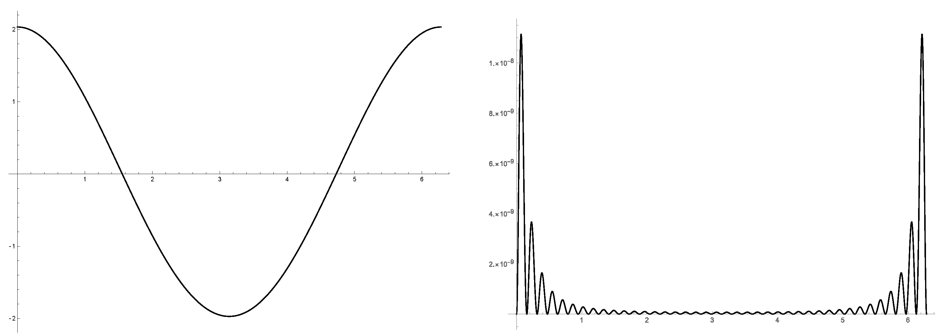
The Cardan transmission is a well-known device, and the equations that govern the angular displacement for the driving and driven shafts can be found in books on mechanics, such as [19] (Section 2.6) and [20]. With ${\Theta }_2\left(t\right)$ denoting the angular displacement of Disk 2 and supposing that ${\Theta }_2\left(0\right)=0$, we can state that:

$${\Theta }_2\left(t\right)=arctan\left(\frac{sin\left(\frac{2\pi t}{T}\right)}{cos\left(\frac{2\pi t}{T}\right)cos\beta }\right)and{w}_2\left(t\right)=\frac{d{\Theta }_2\left(t\right)}{dt}=\frac{2\pi }{T}\frac{cos\beta }{(1-si{n}^2\beta ){cos}^2\left(\frac{2\pi t}{T}\right)}.$$

The last equation above shows one characteristic of the considered Cardan joint: it is not homokinetic. Indeed, $\frac{d{\Theta }_2\left(t\right)}{dt}$ is not constant, and there exist positive numbers A and B, with $B<1$, such that:

$$\begin{array}{c}\hfill (1-B)\frac{2\pi }{T}=cos\beta \frac{2\pi }{T}\le \frac{2\pi }{T}(1-C\left(t\right))=w_2\left(t\right)\le \frac{1}{cos\beta }\frac{2\pi }{T}=(1+A)\frac{2\pi }{T}\end{array}$$

(32)

with $1-C\left(t\right)>0$ and bounded.

On the other hand, we denote the angular displacement of Disk 1 by ${\Theta }_1\left(t\right)$, and if we suppose that ${\Theta }_1\left(0\right)=0$, we have ${\Theta }_1\left(t\right)=\frac{2\pi (n+1)}{T}t$. After $t=T$, the hole of Disk 1 reaches that of Disk 2 n times. Moreover, we can bound the time between two of these events. For $\Delta t$, the angle of displacement for Disk 1 is $\frac{2\pi (n+1)}{T}\Delta t$ and for Disk 2 is $w_2\left(t_1\right)\Delta t$ ($t_1$ is an intermediate value between the t values for both events). Since the first displacement is $2\pi$ radians greater than the second one, we have:

$$\begin{array}{c}\hfill 2\pi =\frac{2\pi (n+1)}{T}\Delta t-w_2\left(t_1\right)\Delta t\Rightarrow \Delta t=\frac{2\pi }{\frac{2\pi (n+1)}{T}-(1-C\left(t_1\right))\frac{2\pi }{T}}=\frac{T}{n+C\left(t_1\right)}\Rightarrow \\ \hfill \Delta t=\frac{T}{n}-\frac{C\left(t_1\right)T}{n(n+C\left(t_1\right))}.\end{array}$$

(33)

In other words, we have:

$$\Delta t=\frac{T}{n}+\mathcal{O}\left(\frac{1}{n^2}\right)=\frac{2\pi }{n}+\mathcal{O}\left(\frac{1}{n^2}\right).$$

When the period is $T\ne 2\pi$, we can change the independent variable t by the new variable $t^{\prime }=\frac{2\pi }{T}t$ and use the previous analysis. As can be seen, holes would only face each other for evenly spaced times for a null angle, that is for homokinetic joints. Notice that the nodal system determined by the events satisfies the separation relation (13).

We must point out that we can use the interpolation scheme on the unit circle to perform trigonometrical interpolation on the interval $[0,2\pi ]$ for periodic functions. The idea is quite similar to that developed in Section 5. Here, we must consider the change $z=e^{i\theta }$; in particular, the change $z=e^{it}$. In this case, the nodal system satisfies (13), and we can confidently use the interpolation methods. To compute the interpolation polynomials, we used the barycentric representation given by (11).

We obtained a nodal system employing for the previous scheme $n=40$ and $\beta =\frac{\pi }{7}$. As a test function, we used ${\displaystyle \sum _{k=1}^{\infty }}\frac{2}{k^6}cos\left(k\theta \right)$ which led to $f\left(z\right)={\displaystyle \sum _{k=1}^{\infty }}\frac{1}{k^6}(z^k+z^{-k})$. The left-hand side in Figure 1 shows the real part of the interpolator along with the interpolated function. We observed that they were indistinguishable. On the right-hand side, we represent the real part of the error. The imaginary parts in both cases are irrelevant.

Example 2.

A certain periodic magnitude of period $T=2\pi$ is observed using a certain measuring device with which n measurements are taken. Each one is intended to be obtained just after a countdown of $\frac{2\pi }{n}$, this time needed for the correct performance of the device. It includes an automatic repair of four possible errors. Every error has a probability of p, and they are independent. Each repair requires a time of $\frac{1}{n^2}$, which can lead to the fact that between two measures, the time is greater than or equal to $\frac{2\pi }{n}$.

Thus, in this case, we cannot ensure evenly spaced measurements. Between two of them, we have $\Delta t=\frac{2\pi }{n}+\frac{A}{n^2}$ where A is random. Indeed, it is a binomial variable $B(4,p)$ and $0\le A\le 4$ in the way that $\Delta t=\frac{2\pi }{n}+\mathcal{O}\left(\frac{1}{n^2}\right)$. Again, the nodal system satisfies the separation property (13).

Naturally, the rest of the ideas of the previous example can be applied. Consequently, we can be confident when using Hermite or Hermite–Fejér interpolation based on the corresponding random nodal systems.

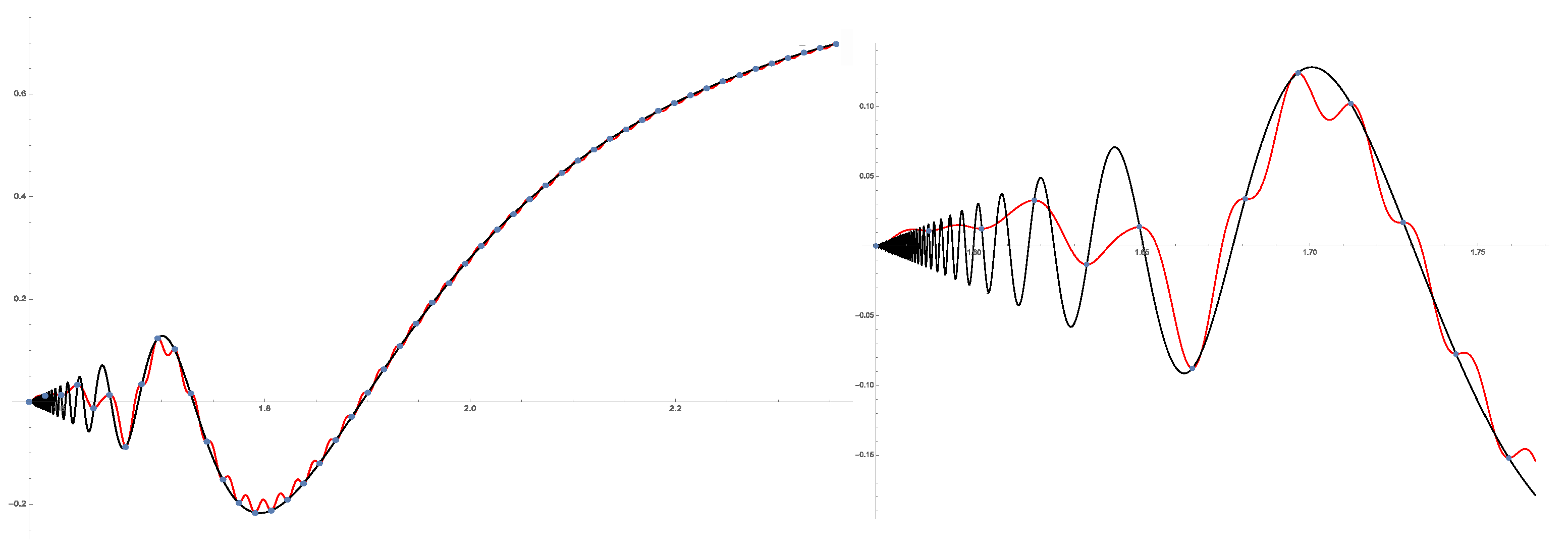
We obtained a particular nodal system using for the previous scheme $n=400$ and $p=0.6$. As a test function, we used the continuous non-derivable function $costsin\left(\frac{1}{cost}\right)$, which led to $f\left(z\right)=\frac{z+\frac{1}{z}}{2}sin\left(\frac{2}{z+\frac{1}{z}}\right)$, and we performed Hermite–Fejér interpolation. To obtain the corresponding interpolator, we used the barycentric formula (12). The left-hand side in Figure 2 shows the real part of the interpolator together with the interpolated function on $[\frac{\pi }{2},\frac{3\pi }{4}]$. On the right-hand side, we represent the same pair in a quite small interval. We point out the characteristic shape of the Hermite–Fejér interpolation on the nodes. The imaginary parts in both cases are irrelevant.

Example 3.

An artificial satellite takes measurements of a periodic phenomenon of period $T_1$ that has its origin at the point at infinity of the perpendicular to its elliptical orbit of period T around a star. The satellite can rotate on itself, and it can vary its speed of rotation, although not its orbit. The orbit was intended to be circular, but ended up being elliptical. Observations have to be taken when one particular point of the satellite is in its solar noon, that is when the center of the star, the center of the satellite, and the point are aligned (event).

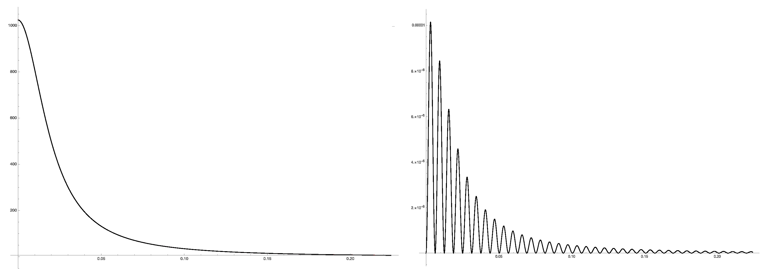
In this scenario, we can successfully apply the ideas in Section 4. Let us suppose that at Time 0, the satellite is at its aphelion and at its solar noon. By using the laws of the two-body problem, we can know its true anomaly ϕ at time $T_1$ and adjust the rotation of the satellite so that the point is at its $\left(n\right)$ solar noon, having rotated $(n+1)2\pi +\varphi$. Logically, the time lapse between two solar noons would be equal if the orbit were circular. However, as a consequence of Kepler’s second law, the rate of variation of the angular velocity of the satellite (in orbit) $w_1$ is a variable that oscillates between the values that it takes at aphelion and perihelion. Note that if $T_1=T$, the satellite would rotate at an angular speed of $\frac{2\pi (n+1)}{T}$ leading to Equation (29). Furthermore, $C\left(t\right)$ would be bounded, the mean $w_1$ value being $\frac{2\pi }{T}$. Thus, it is possible to ensure that the times between the satellite noons are variable, but with the form $\frac{T_1}{n}+\mathcal{O}\left(\frac{1}{n^2}\right)$, that is the nodal system fulfills Relation (13). Using the new variable $t^{\prime }$ given by $t^{\prime }=\frac{2\pi }{T_1}t$, we have a Hermite or Hermite–Fejér interpolation problem based on a nodal system satisfying (13). Hence, we can use the mechanism.

When determining the noon of the satellite, we must use some elements of the mechanics of elliptical orbits. The ideas are quite similar to those of Example 1. However, in this case, we must use equations related to elliptical orbits. The true anomaly is determined by t, T and the eccentricity of the orbit e. The algorithm can be found in [21] (Chapter 3, Section 4).

We obtained a particular nodal system using the previous scheme with $n=1000$, $e=0.25$, and for simplicity, $T_1=T=$ 8,640,000. We used $\frac{1}{[1+{\left(1.02\right)}^2-2.04cos\theta ][1+{\left(1.2\right)}^2+2.4sin\theta ]}$ as the test function, which led to $f\left(z\right)=\frac{1}{(z-1.02)(\frac{1}{z}-1.02)(z+1.2ı)(\frac{1}{z}-1.2ı)}$. The left-hand side in Figure 3 shows the real part of the interpolator with the interpolated function near $z=1$, the most problematic area. We obtained the interpolator by using the formula (11). We observed that they were indistinguishable. On the right-hand side, we represent the real part of the error. The imaginary parts in both cases are irrelevant.

7. Notation

Next, we summarize the notation related to the polynomials used throughout the paper:

$W_n\left(z\right)={\prod }_{j=1}^n(z-{\alpha }_j)$ is the nodal polynomial.

The Laurent polynomials of Hermite interpolation are denoted by:

${\mathcal{H}}_{-n,n-1}\left(z\right)$ for the values ${\left\{u_j\right\}}_{j=1}^n$ and ${\left\{v_j\right\}}_{j=1}^n.$

${\mathcal{HF}}_{-n,n-1}\left(z\right)$ for the values ${\left\{u_j\right\}}_{j=1}^n$ and ${\left\{0\right\}}_{j=1}^n.$

${\mathcal{HD}}_{-n,n-1}\left(z\right)$ for the values ${\left\{0\right\}}_{j=1}^n$ and ${\left\{v_j\right\}}_{j=1}^n.$

Clearly, ${\mathcal{H}}_{-n,n-1}\left(z\right)={\mathcal{HF}}_{-n,n-1}\left(z\right)+{\mathcal{HD}}_{-n,n-1}\left(z\right).$

${\mathcal{H}}_{-n,n-1}(f,z)$ for the values ${\left\{f\left({\alpha }_j\right)\right\}}_{j=1}^n$ and ${\left\{f^{\prime }\left({\alpha }_j\right)\right\}}_{j=1}^n.$

${\mathcal{HF}}_{-n,n-1}(f,z)$ for the values ${\left\{f\left({\alpha }_j\right)\right\}}_{j=1}^n$ and ${\left\{0\right\}}_{j=1}^n.$

${\mathcal{HD}}_{-n,n-1}(f,z)$ for the values ${\left\{0\right\}}_{j=1}^n$ and ${\left\{f^{\prime }\left({\alpha }_j\right)\right\}}_{j=1}^n.$

Clearly, ${\mathcal{H}}_{-n,n-1}(f,z)={\mathcal{HF}}_{-n,n-1}(f,z)+{\mathcal{HD}}_{-n,n-1}(f,z).$

${\mathcal{H}}_{-n,n-1}(f,{\gamma }_n,z)$ for the values ${\left\{f\left({\alpha }_j\right)\right\}}_{j=1}^n$ and ${\left\{v_j\right\}}_{j=1}^n,$ where ${\gamma }_n={\left\{v_j\right\}}_{j=1}^n.$

8. Materials and Methods

To perform the three numerical experiments (arrays, interpolators, and plots) included in the previous section, we used the formulae included in the paper, and we elaborated three programs that could be obtained, with public access, at the url https://www.dropbox.com/sh/0cx9chq3jfzov2w/AAA_SvL2i7HlC7ChMGpuG-Ata?dl=0 (accessed on 22 March 2021). Actually, these programs are notebooks (files with the names cardan, kepler, and random, which have as the extension .nb) elaborated with Mathematica (Mathematica is a trademark property of Wolfram Research). Mathematica is a quite standard software for mathematical computing. In particular, we used Version 12 Release 2. We do not hesitate to state that the programs (notebooks) run correctly in recent previous versions and in future versions because we used quite simple commands. Moreover, we did not use compiled routines nor other software.

9. Discussion

The nodal systems usually used for interpolation problems on the real line and the unit circle are related to measures. Normally, the zeros of orthogonal or para-orthogonal polynomials with respect to measures on the real line or the circumference, respectively, are considered as nodal points.

In the previous paper [9], new nodal systems were introduced, which in the case of the circumference proceeded from a perturbation of the roots of unity. Moreover, the Lagrange interpolation theory based on these nodal points was developed. In [9], the study of other types of interpolation was also suggested by using these nodal arrays as a future new research line. By following this idea, in the present paper, we developed the corresponding Hermite polynomial interpolation theory on the circle, as well as on the bounded interval.

The new nodal systems, whose study was completed in this paper, are very suitable to solve Hermite interpolation problems that appear in practice, most of which are linked to interesting mechanical models.

These nodal systems have not been used before in the Hermite interpolation due to the lack of a convergence theory to support their use. Thus, in this article, we dedicated a section to the study of the convergence of Hermite–Fejér interpolants in the case of continuous functions and the convergence of Hermite interpolants for smooth functions. With the theory developed in this paper, we are in conditions to use these nodal distributions for those models that fit to them. Taking into account these ideas, we presented three mechanical models for which the application of our results is very suitable.

The nodal system of the first example appeared as a consequence of a Cardan movement. We used the Hermite scheme given in Section 4.2 to recover an analytic function. The nodal system of the second example was a consequence of a random process. In this case, we used the Hermite–Fejér interpolator to approximate a quite variable continuous function. The convergence of this process is guaranteed by the results in Section 4.1. The last example is linked to a planetarium movement and to recovering a smooth non-analytic function following Section 4.2. Clearly, the examples only pretend to visualize the theoretical results previously obtained.

A possible future research line connected with this work could be the study of the corresponding Gibbs–Wilbraham phenomena.