Article

Numerical Solution of Bending of the Beam with Given Friction

by
Michaela Bobková
and
Lukáš Pospíšil
*
Department of Mathematics, Faculty of Civil Engineering, VSB-TU Ostrava, Ludvíka Podéště 1875/17, 708 00 Ostrava, Czech Republic
*
Author to whom correspondence should be addressed.
Mathematics 2021, 9(8), 898; https://doi.org/10.3390/math9080898
Submission received: 19 March 2021 / Revised: 13 April 2021 / Accepted: 15 April 2021 / Published: 18 April 2021
(This article belongs to the Special Issue Numerical Analysis and Scientific Computing)

Abstract

:
We are interested in a contact problem for a thin fixed beam with an internal point obstacle with possible rotation and shift depending on a given swivel and sliding friction. This problem belongs to the most basic practical problems in, for instance, the contact mechanics in the sustainable building construction design. The analysis and the practical solution plays a crucial role in the process and cannot be ignored. In this paper, we consider the classical Euler–Bernoulli beam model, which we formulate, analyze, and numerically solve. The objective function of the corresponding optimization problem for finding the coefficients in the finite element basis combines a quadratic function and an additional non-differentiable part with absolute values representing the influence of considered friction. We present two basic algorithms for the solution: the regularized primal solution, where the non-differentiable part is approximated, and the dual formulation. We discuss the disadvantages of the methods on the solution of the academic benchmarks.

1. Introduction

Mathematical modeling plays a crucial role in the simulations and the development of sustainable civil engineering. This paper aims to present the whole story of the solution process of a given problem, instead of focusing only on one specific step of the solution process. Additionally, we would like to show that in the case of practical computation, in the end, the numerical solver always matters. Indeed, even though the solver has to be chosen in a convenient way referring to the properties of the given problem, the efficiency of the solution crucially depends on the choice of the right numerical approach; actually, there will always be pros and cons, which have to be taken into the consideration.
In the paper, we examine this rule on algorithms for the numerical solution of the beam bending problem of a thin fixed beam with an internal point obstacle with possible rotation and shift depending on a given swivel and sliding friction. The beam is a structural element that primarily resists loads applied laterally to the axis. In the case of a thin beam, we suppose that the diameter of the cross section is much smaller than the length of the beam. The thin fixed beam considered in this paper is the thin beam fixed on both sides.
We suppose that the length of the beam is much bigger than its height. The considered load function applies to small deflections of a beam without considering the effects of shear deformations. Such an example belongs to the most popular benchmarks in engineering practice because of its linearity, and it is well known as the Euler–Bernoulli beam model (see, e.g., in [1], where authors present the derivation of the model). For the nonlinear beam model, which supposes large deformations, we can choose, for example, the Gao beam model, which has been originally proposed in [2]. The model is commonly used both in practice and theory, for example, the extension for contact problems with obstacle [3], friction [4], the extension incorporating nonlocality and surface energy effect [5], or the application to optimal control [6].
From the mathematical point of view, the classical formulation of the problem is represented as a linear differential equation of the fourth-order with corresponding additional conditions. In this case, the weak formulation is defined as an elliptical variational inequality of the second type with non-differentiable functional. For more details see, e.g., the comprehensive books in [7,8,9]. In this paper, we shortly review the formulation in Section 2.1, where we also shortly discuss the existence and uniqueness of the solution in the case of the continuous formulations and the approximated problem.
Convergence analysis and an algebraic formulation is presented in Section 2.4. To solve the problem numerically, we adopt the Finite Element Method (FEM) with Hermite spline functions (see, e.g., the introductory book in [10] or the comprehensive numerical analysis in [11]), see Section 2.6.
Two methods are used to solve the problem in Section 2.7. The first one is the method of regularization, which is based on the approximation of the non-differentiable functional by the differentiable one. The second approach is the dualization of the problem and its reformulation into the so-called Quadratic programming (QP) problem [12]. The corresponding dual problem in our case is a minimization of a strictly convex quadratic function on a feasible set defined by box constraints.
As an example of the presented theory and methods of solution, we consider three benchmarks with increasing difficulty, see Section 2.8. These benchmarks show the basic properties of adopted numerical approaches. The results are discussed in Section 3.
Finally, Section 4 concludes the paper. Please see the section titled “Appendix A” for the list of notations used in the paper.

2. Materials and Methods

2.1. Problem Formulation

We consider a thin fixed beam of length l > 0 with special internal point obstacle x ^ with possible shift and rotation depending on a given sliding g 1 0 and swivel g 2 0 friction, see Figure 1. The geometry of the beam is defined by the moment of inertia of the cross section J ( x ) , x [ 0 , l ] , and the material of the body is defined by Young’s modulus of elasticity E ( x ) . The problem is to find the deflection of the beam u, which is caused by the load function f and limited by the considered type of obstacle.

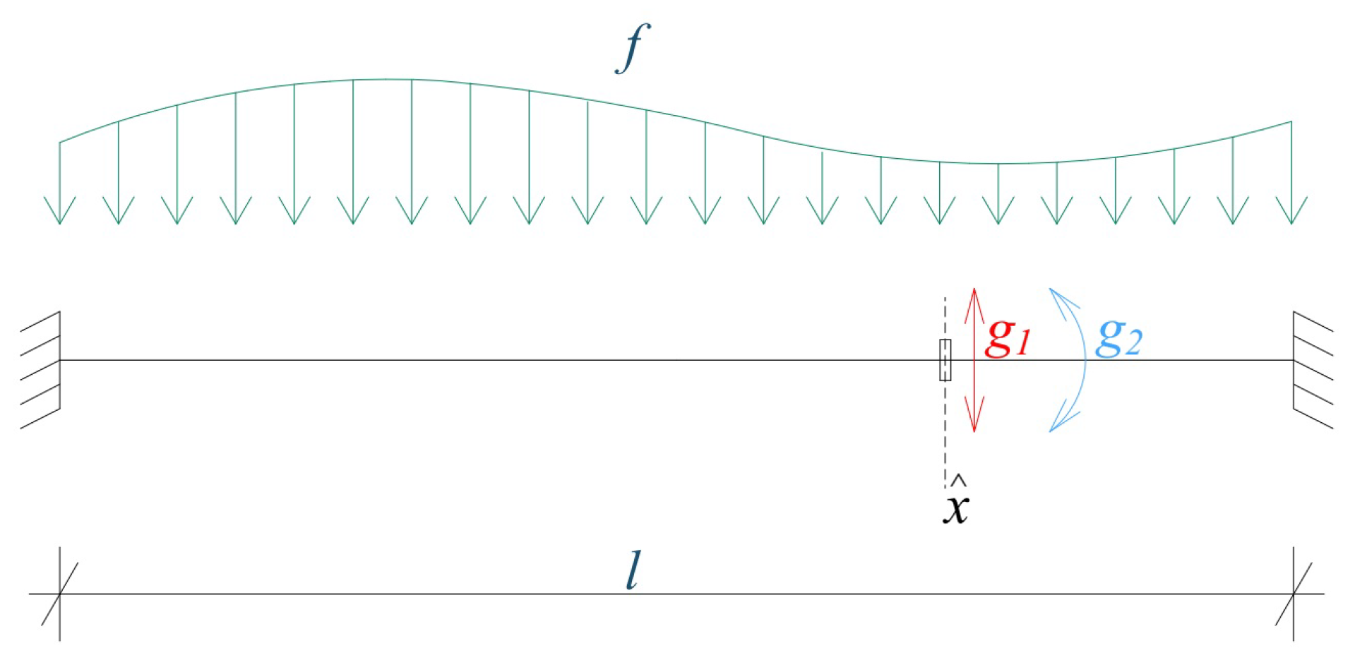
2.2. Classical Formulation of the Problem

To introduce the continuous classical formulation, we assume a beam of length l R + , load function f C ( ( 0 , l ) ) , E , J C 2 ( ( 0 , l ) ) , and internal point obstacle x ^ ( 0 , l ) , given sliding friction g 1 0 and given swivel friction g 2 0 . We consider the following problem: find a function u, such that
( P T M ) u C 4 ( ( 0 , l ) ) : D 2 ( E ( x ) J ( x ) D 2 u ( x ) ) = f ( x ) x ( 0 , l ) ,
u ( 0 ) = D u ( 0 ) = u ( l ) = D u ( l ) = 0 ,
| ( T T + ) ( u ( x ^ ) ) | g 1 ,
g 1 | u ( x ^ ) | + ( T T + ) ( u ( x ^ ) ) u ( x ^ ) = 0 ,
| ( M M + ) ( u ( x ^ ) ) | g 2 ,
g 2 | D u ( x ^ ) | + ( M M + ) ( u ( x ^ ) ) D u ( x ^ ) = 0 .
Function u, corresponding to the problem ( P T M ) , will be called a classical solution of the considered problem.
The differential equation (1) is a mathematical model of the bending of the Euler–Bernoulli beam. The boundary conditions (2) define the clamping of the beam at both ends, relations (3) and (4) represent the conditions of given sliding friction, and relations (5) and (6) are the conditions of the given swivel friction.

2.3. Weak and Variational Formulation

As the classical formulation of the problem is too strong and therefore not suitable for direct numerical solution, we formulate the considered problem as a variational one.
Let f L 2 ( ( 0 , l ) ) , g i 0 , i = 1 , 2 , and E , J L ( ( 0 , l ) ) . We define the space V of test functions, corresponding to the boundary conditions, as a Sobolev space (see, e.g., in [11,13]) as follows:
V = H 0 2 ( ( 0 , l ) ) .
Let us denote
q 1 ( v ) = g 1 | v ( x ^ ) | , q 2 ( v ) = g 2 | D v ( x ^ ) | .
Next, we introduce the functional q : V R ¯ , corresponding to given swivel and sliding frictions, in the form
q ( v ) = q 1 ( v ) + q 2 ( v ) .
Using (8), we have
q ( v ) = g 1 | v ( x ^ ) | + g 2 | D v ( x ^ ) | .
Let u be a solution of the problem ( P T M ) and v V . By scalar multiplication of Equation (1) by the function v u and integration (using Green’s theorem—see, e.g., [14]) on the interval ( 0 , l ) , we obtain
0 l D 2 ( E ( x ) J ( x ) D 2 u ( x ) ) ( v u ) ( x ) d x = 0 l E ( x ) J ( x ) D 2 u ( x ) D 2 ( v u ) ( x ) d x + ( T T + ) ( u ( x ^ ) ) ( v u ) ( x ^ ) + ( M M + ) ( u ( x ^ ) ) D ( v u ) ( x ^ ) =
= 0 l f ( v u ) ( x ) d x v V .
From (4) and (6), we have
( T T + ) ( u ( x ^ ) ) u ( x ^ ) = | u ( x ^ ) | g 1 ,
( M M + ) ( u ( x ^ ) ) D u ( x ^ ) = | D u ( x ^ ) | g 2 .
Using (12), (13) and (3), (5), it follows from (11) that
0 = 0 l D 2 ( E ( x ) J ( x ) D 2 u ( x ) ) ( v u ) ( x ) d x 0 l f ( v u ) ( x ) d x = = 0 l E ( x ) J ( x ) D 2 u ( x ) D 2 ( v u ) ( x ) d x ( T T + ) ( u ( x ^ ) ) v ( x ^ ) + + ( T T + ) ( u ( x ^ ) ) u ( x ^ ) + ( M M + ) ( u ( x ^ ) ) D v ( x ^ ) + ( M M + ) ( u ( x ^ ) ) D u ( x ^ ) 0 l f ( v u ) ( x ) d x 0 l E ( x ) J ( x ) D 2 u ( x ) D 2 ( v u ) ( x ) d x + | ( T T + ) ( u ( x ^ ) ) | | v ( x ^ ) | + | u ( x ^ ) | g 1 + | ( M M + ) ( u ( x ^ ) ) | | D v ( x ^ ) | + | D u ( x ^ ) | g 2 0 l f ( v u ) ( x ) d x 0 l E ( x ) J ( x ) D 2 u ( x ) D 2 ( v u ) ( x ) d x + | v ( x ^ ) | g 1 | u ( x ^ ) | g 1 + + | D v ( x ^ ) | g 2 | D u ( x ^ ) | g 2 0 l f ( v u ) ( x ) d x v V .
Afterwards, we can define a weak formulation of the problem ( P T M ) as a problem of finding a function u such that
( P T M ) u V : a ( u , v u ) + q ( v ) q ( u ) F ( v u ) v V ,
where
a ( u , v ) = 0 l E ( x ) J ( x ) D 2 u ( x ) D 2 v ( x ) d x ,
F ( v ) = ( f , v ) = 0 l f v ( x ) d x .
The sought function u is a weak solution of the problem ( P T M ) .
Remark 1.
The weak formulation ( P T M ) of the problem ( P T M ) is formulated as an elliptical variational inequality of the second type with non-differentiable functional q (see, e.g., in [8]).
Let form a : V × V R and functional F : V R be given by relations (15) and (16) and f L 2 ( ( 0 , l ) ) , E , J L ( ( 0 , l ) ) such that
E ( x ) E 0 > 0 a l m o s t e v e r y w h e r e o n ( 0 , l ) ,
J ( x ) J 0 > 0 a l m o s t e v e r y w h e r e o n ( 0 , l ) .
Obviously, the form a is bilinear and symmetric. To prove its continuity we use Hölder’s inequality (see, e.g., in [7])
| a ( u , v ) | = | 0 l E ( x ) J ( x ) D 2 u ( x ) D 2 v ( x ) d x | c 0 l | D 2 u ( x ) | | D 2 v ( x ) |
c ( 0 l | D 2 u ( x ) | 2 ) 1 2 ( 0 l | D 2 v ( x ) | 2 ) 1 2 c ˜ u H 2 v H 2 v , u V ,
where c = E L J L . From the assumptions (17) and (18) of functions E, J and from v 2 ( 0 ) = 0 , we have
a ( v , v ) = 0 l E ( x ) J ( x ) ( D 2 v ( x ) ) 2 d x E 0 J 0 ( 0 l ( D 2 v ( x ) ) 2 d x + v 2 ( 0 ) ) .
Here, we apply Friedrichs’s inequality (see, e.g., [7]) to obtain the V-ellipticity of the form a
a ( v , v ) E 0 J 0 k v H 2 2 = c v H 2 2 v V ,
where c = E 0 J 0 k > 0 and k is the positive constant from Friedrichs’s inequality. It is also clear that the functional F is linear. Using Cauchy–Schwarz inequality (see, e.g., in [7]), we can prove its continuity, i.e., F V * .
Let t ( 0 , 1 ) . Then, for functional q given by (10), it holds that
q ( 1 t ) v + t u = g 1 | ( 1 t ) v ( x ^ ) + t u ( x ^ ) | + g 2 | D [ ( 1 t ) v ( x ^ ) + t u ( x ^ ) ] |
( 1 t ) g 1 | v ( x ^ ) | + t g 1 | u ( x ^ ) | + ( 1 t ) g 2 | D v ( x ^ ) | + t g 2 | D u ( x ^ ) | =
= ( 1 t ) [ g 1 | v ( x ^ ) | + g 2 | D v ( x ^ ) | ] + t [ g 1 | u ( x ^ ) | + g 2 | D u ( x ^ ) | ] =
= ( 1 t ) j ( v ) + t j ( u ) ,
which means that q is convex. Immediately from the definition of q, we can see that q ( v ) 0 > v V . Moreover, for zero function v V , it holds q ( v ) = 0 , i.e., q ( V ) and thus q is proper on V. It is clear that the functional q is continuous. The convexity and continuity of q imply its semi-continuity from below. Therefore, the existence and uniqueness of the solution of problem ( P T M ) are guaranteed by the following Theorem 1, the assumptions of which are thus fulfilled.
Theorem 1.
Let a : V × V R be bounded, V-elliptical bilinear form, F V * and let functional j : V R ¯ be convex, semi-continuous from below and proper on V. Then, there exists an unique solution of
a ( u , v u ) + j ( v ) j ( u ) F ( v u ) v V .
For more detail, see, e.g., in [8,15].
As a is bounded; the V-elliptical is bilinear and of symmetric form; functional q is convex, semi-continuous from below, and proper on V; and the problem ( P T M ) is equivalent to the variational problem of minimizing quadratic energy functional, i.e.,
( P ^ T M ) u V : u = arg min v V J ( v ) ,
where
J ( v ) = 1 2 a ( v , v ) + q ( v ) F ( v ) .

2.4. Approximation

Let f L 2 ( ( 0 , l ) ) and E , J L ( ( 0 , l ) ) satisfy relations (17) and (18), respectively. Let the form a : V × V R and the functional F : V R be given by (15) and (16), respectively. We consider a system of partitions { D h } , h 0 + of the interval [ 0 , l ] into subintervals
T k ( h ) = [ x k ( h ) 1 , x k ( h ) ] , k ( h ) = 1 , , n ( h )
such that points x i , i = 1 , , n ( h ) 1 are nodal points, i.e.,
0 = x 0 < x 1 ( h ) < < x n ( h ) = l D h ,
where n ( h ) + 1 is the number of nodal points of D h and h is the maximum length of intervals T k ( h ) . Moreover, the point obstacle x ^ D h for any h. We define the following finite-dimensional subspace V h V :
V h = { v h C 1 ( [ 0 , l ] ) : v h | T k ( h ) P 3 T k ( h ) D h , v h ( 0 ) = D v h ( 0 ) = v ( l ) = D v ( l ) = 0 } D h .
Therefore, spaces V h satisfy classical boundary conditions and additionally
dim V h = m ( h ) < , where m ( h ) = 2 ( n ( h ) 1 )
and
lim h 0 + dim V h = lim h 0 + m ( h ) = .
We approximate the functional q for each h by functional q h : V h R ¯ by
q h ( v h ) = g 1 | v h ( x ^ ) | + g 2 | D v h ( x ^ ) | .
Functional q h is convex, semi-continuous from below and proper in the space V h . We can approximate problem ( P T M ) by the sequence of problems of finding u h such that
( P T M ) h u h V h : a ( u h , v h u h ) + q h ( v h ) q h ( u h ) F ( v h u h ) v h V h .
The existence and uniqueness of the solution of ( P T M ) h is guaranteed by the Theorem 1.
As the form a is symmetric, the problem ( P T M ) h is equivalent to the problem of finding u h such that
( P ^ T M ) h u h V h : u h = arg min v h V h J h ( v h ) ,
where
J h ( v h ) = 1 2 a ( v h , v h ) F ( v h ) + q h ( v h ) .
To approximate the function v H 2 ( ( 0 , l ) ) , we use the Hermitian cubic spline function for each D h such that
v h ( x i ) = v ( x i ) , D v h ( x i ) = D v ( x i ) x i D h , v H 2 ( ( 0 , l ) ) .
Additionally,
lim h 0 + v h = v v H 2 ( ( 0 , l ) ) .
Remark 2.
For the given function v H 2 ( ( 0 , l ) ) , the Hermitian cubic spline function is given by
v h ( x ) = v ( x k ) [ 2 ( x k x ) ( x k + 1 x k ) ] ( x x k + 1 ) 2 ( x k x k + 1 ) 3 + D v ( x k ) ( x x k ) ( x x k + 1 ) 2 ( x k + 1 x k ) 2 + + v ( x k + 1 ) [ 2 ( x k + 1 x ) ( x k + 1 x k ) ] ( x x k ) 2 ( x k x k + 1 ) 3 + D v ( x k + 1 ) ( x x k + 1 ) ( x x k ) 2 ( x k + 1 x k ) 2 , x [ x k , x k + 1 ] , k = 0 , . . . , n ( h ) 1 .

2.5. Convergence Analysis

To prove the convergence of the approximated solutions u h to the weak solution u of the considered problem, we use the following theorem.
Theorem 2.
Let a : V × V R be bounded, V-elliptical bilinear form on V. Let there exist operator r h : X V h such that
r h v v f o r h 0 + v X ,
where X V such that X ¯ = V . Let the system of functionals j h meet the following two conditions:
v h v , v h V h lim inf h 0 + j h ( v h ) j ( v ) ,
lim h 0 + j h ( r h v ) = j ( v ) v X .
Then, it holds that
u u h V 0   f o r   h 0 + .
Moreover,
lim h 0 + j h ( u h ) = j ( u ) .
For more details, see, e.g., in [16].
As the functional q h is convex and semi-continuous from below on V h , it is also weakly semi-continuous from below. In our case, operators r h are operators of the appropriate Hermitian interpolation. From the (28), it follows that
q h ( v h ) = q ( v ) v V .
Therefore,
lim h 0 + q h ( r h v ) = q ( v ) v V .
This means that assumptions of Theorem 2 are satisfied, i.e., the sequence u h of solution approximations of the problem ( P T M ) h converges to the solution u of the problem ( P T M ) in the V-space norm.

2.6. The Algebraic Formulation

Let the form a and the functional F be defined by (15) and (16), respectively. We choose a finite-dimensional space V h , dim V h = N with N = 2 ( n ( h ) 1 ) . Let { φ i } , i = 1 , , N be a basis of V h chosen by FEM, i.e., i , j = 1 , . . . , n ( h ) 1
φ 2 i 1 ( x j ) = δ i j ; φ 2 i ( x j ) = 0 ; D φ 2 i 1 ( x j ) = 0 ; D φ 2 i ( x j ) = δ i j .
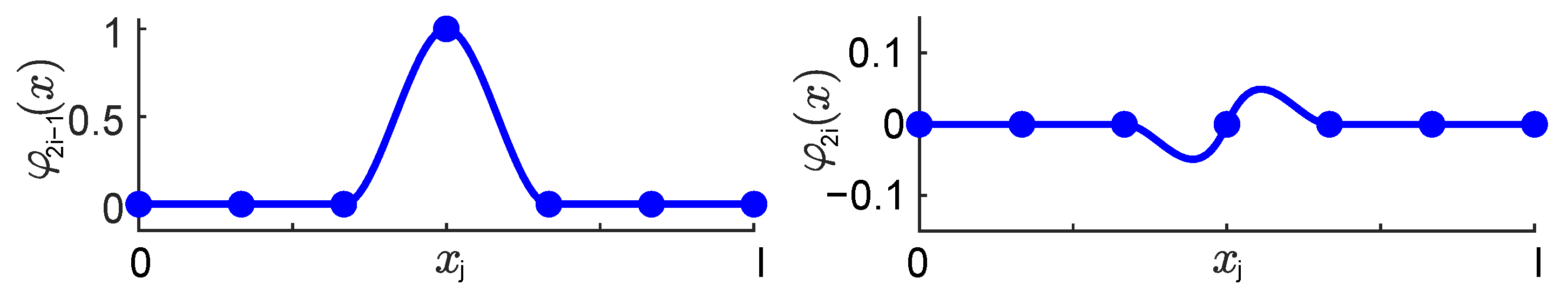
To obtain a shape of basis functions, we apply the Hermite’s cubic splines. We have
φ 2 i ( x ) = 0 x [ x i 1 , x i + 1 ] , ( x x i ) 3 ( x i 1 x i ) 2 2 ( x x i ) 2 x i 1 x i + ( x x i ) x [ x i 1 , x i ] , ( x x i ) 3 ( x i + 1 x i ) 2 2 ( x x i ) 2 x i + 1 x i + ( x x i ) x [ x i , x i + 1 ] ,
φ 2 i 1 ( x ) = 0 x [ x i 1 , x i + 1 ] , 1 + 2 ( x x i x i 1 x i ) 3 3 ( x x i x i 1 x i ) 2 x [ x i 1 , x i ] , 1 + 2 ( x x i x i + 1 x i ) 3 3 ( x x i x i + 1 x i ) 2 x [ x i , x i + 1 ] .
For an example of geometric representation, please see Figure 2.
Any function v h V h can be uniquely written in the form of linear combination of basis functions, i.e.,
v h = i = 1 N c i φ i ,
where c i R are the corresponding coordinates of v h in the basis. It is clear that φ i , c i depend on h. If we substitute v h from (33) into the functional J h given by (27), we obtain
J h ( v h ) = J h ( k c k φ k ) = 1 2 a ( k c k φ k , j c j φ j ) F ( k c k φ k ) +
+ q h ( k c k φ k ) = 1 2 k j c k c j a ( φ k , φ j ) k c k F ( φ k ) +
+ q h ( k c k φ k ) = 1 2 ( c , A c ) + q h ( Φ , c ) ( b , c ) ,
where
  • A = ( a k j ) k , j = 1 N is a stiffness matrix with elements a k j = a ( φ k , φ j ) ,
  • b = ( b 1 , , b N ) is a vector of right-hand sides with elements b i = F ( φ i ) ,
  • c = ( c 1 , , c N ) is a vector of unknown coefficients of linear combination (33),
  • Φ = ( φ 1 , . . . , φ N ) is vector of base functions φ i , i = 1 , . . . , N .
Functional J h is expressed as a quadratic function of variables c 1 , , c N . Let us define an isomorphism T : V h R N by relation
T v h = c = ( c 1 , , c N ) R N v h V h .
Then, the problem ( P ^ T M ) h can be rewritten in the equivalent form where it is required to find c * such that
( P ^ T M ) N c * R N : c * = arg min c R N J ˜ h ( c ) ,
where
J ˜ h ( c ) = J h ( T 1 c ) = 1 2 ( c , A c ) + q h ( Φ , c ) ( b , c ) ,
q h ( Φ , c ) = g 1 | c 2 j ^ 1 | + g 2 | c 2 j ^ | ,
T 1 is inverse of T , and j ^ is index of the nodal point x j ^ = x ^ .
Problem ( P ^ T M ) N is the algebraic form of problem ( P ^ T M ) h .

2.7. Numerical Realization

In this section, we examine two different approaches for the practical numerical solution of the problem. For simplicity, we consider an equidistant grid
0 = x 0 < x 1 < < x n = l , x j = j h , j = 0 , , n ,
where n + 1 is a number of nodal points and h = l / n is a size of intervals. Following the Ritz–Galerkin method, we approximate V by finite-dimensional space
V h = { v h C 1 ( [ 0 , l ] ) : v h | [ x j , x j + 1 ] P 3 j = 0 , , n 1 and v h ( 0 ) = D v h ( 0 ) = v h ( l ) = D v h ( l ) = 0 } .
Additionally, we assume that there exists j ^ such that x ^ = x j ^ , i.e., the point with defined conditions (3)–(6) is one of the used nodal points.
Remark 3.
Note that dim V h = N = 2 ( n 1 ) because the solution in boundary points is given by conditions (2).
The optimization problem ( P ^ T M ) N can be written in the form
( P ˜ T M ) N c * = arg min c R N J ˜ N ( c ) , J N ˜ ( c ) = ψ ( c ) + q N ( c )
with
ψ ( c ) = 1 2 c T A c b T c , q N ( c ) = g 1 | c 2 j ^ 1 | + g 2 | c 2 j ^ | ,
symmetric positive definite (SPD) matrix A R N , N , and vector b R N .
The solution c * R N of (38) represents the coordinates (33) of unknown discretized deflection u h in the considered basis.
Although the problem (38) has a simple structure, we are still dealing with a nonlinear optimization problem with a non-differentiable objective function. In our case, we are dealing with absolute values in q N ( c ) (39). The optimization problems with absolute values in objective functions arise in various applications, and they are already well examined. For example, when one uses L1-regularization (i.e., so-called least absolute shrinkage and selection operator-LASSO [17]) for regularization of linear regression, the problem has a similar form to (38).
Generally, there exist two types of numerical methods to solve the problem-approximation of a non-differentiable term in objective function or dualization of the problem.

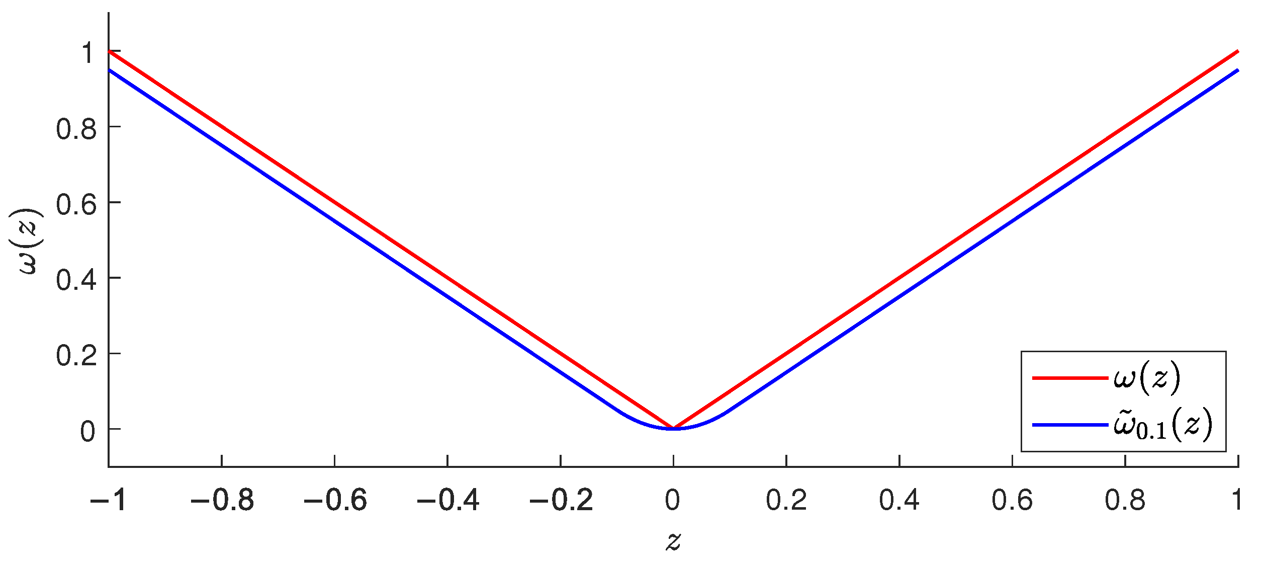
2.7.1. Method of Regularization

The idea is to replace (approximate) the non-differentiable term in objective function with a more suitable differentiable one. In our case, we decided to use the piecewise quadratic approximation, i.e., we approximate absolute value ω ( z ) = | z | by
ω ˜ ε ( z ) = z ε 2 if z < ε , z 2 2 ε if z [ ε , ε ] , z ε 2 if z > ε ,
where ε > 0 is a sufficiently small regularization parameter. The example of this approximation is presented in Figure 3. The derivative is given by
ω ˜ N , ε ( z ) = 1 if z < ε , z ε if z [ ε , ε ] , 1 if z > ε .
Using this approximation, the non-differentiable function q N ( Φ , c ) (39) can be written in form
q ˜ N , ε ( c ) = g 1 ω ˜ ε ( c 2 j ^ 1 ) + g 2 ω ˜ ε ( c 2 j ^ ) .
AS we use piecewise quadratic approximation (40), the derivative is piecewise linear function (41). Additionally, the gradient of quadratic function ψ (39) is linear, and consequently the necessary optimality condition for unconstrained optimization problem (38) is given by the system of linear equations
A c b + q ˜ N , ε ( c ) = 0 .
The components of gradient q ˜ N , ε ( c ) R N are equal to zero except for the components corresponding to partial derivatives of c 2 j ^ 1 and c 2 j ^ . These values depend on conditions from definition of (40) with respect to values c 2 j ^ 1 and c 2 j ^ . The values are presented in Table 1.
The final system of linear equations can be written in form
A ^ c = b ^ ,
where A ^ is a matrix A with diagonal elements modified by coefficients of linear terms in q ˜ N , ε and b ^ is a vector b with additional constant terms from q ˜ N , ε .
It is necessary to solve the problem for all possible cases with respect to c 2 j ^ 1 , c 2 j ^ . The solution of the problem ( P ^ T M ) N (38) is the vector c , for which the corresponding condition on c 2 j ^ 1 , c 2 j ^ with respect to ε is satisfied.

2.7.2. Dual Problem

The idea of this approach is based on simple observation of the following equivalent form of absolute value:
α R + x R : α | x | = max α λ α λ x .
Using this identity, we can rewrite the function q N ( Φ , c ) (39) into
q N ( Φ , c ) = ψ ( c ) + max g 1 λ 1 g 1 λ 1 c 2 j ^ 1 + max g 2 λ 2 g 2 λ 2 c 2 j ^ = max g λ g λ T B c ,
where we denoted
λ = λ 1 λ 2 , g = g 1 g 2 ,
B R 2 , N : B 1 , i = 1 if i = 2 j ^ 1 , 0 elsewhere , and B 2 , i = 1 if i = 2 j ^ , 0 elsewhere .
Using the separability of variables and the saddle-point property [12], we can write optimization problem (38) in equivalent form
min ψ ( c ) + max g λ g λ T B c = min max g λ g ψ ( c ) + λ T B c = max g λ g min ψ ( c ) + λ T B c = L ( c , λ ) .
Function L : R N × 2 R can be considered as a Lagrange function. From the first Karush–Kuhn–Tucker optimality condition [18], we can derive (note that A is SPD, i.e., non-singular)
c L ( c , λ ) = ψ ( c ) + B T λ = A c b + B T λ = 0 c = A 1 ( b B T λ )
and substitute into objective function L to get (for more details see in [19])
1 2 c T A c b T c + λ T B c = 1 2 λ T B A 1 B T λ + λ T B A 1 b 1 2 b T A 1 b .
As the original problem (47) is a maximization problem, we can change the sign of the objective function to obtain
λ * = arg min g λ g 1 2 λ T A ^ λ b ^ T λ , A ^ = B A 1 B T , b ^ = B A 1 b .
Please, notice that the dual problem (49) is a minimization of a strictly convex quadratic function on a feasible set defined by box constraints. Such a problem always has a unique solution [12]. The dimension of the problem is 2, which is much more lower number then the dimension of original primal problem (38). Moreover, the problem belongs to the most basic nonlinear optimization problems and it is solvable by several types of methods, for example, Interior Point, Active set, or Projected Gradient methods [18].

2.8. Numerical Experiments

As a demonstration of the presented theory and methods of solution, we consider three numerical benchmarks: with analytical solution (Benchmark 1), with non-trivial load function (Benchmark 2), and with more internal points with given sliding and swivel friction (Benchmark 3).
Benchmark 1
We consider a most simple case: we suppose problem ( P T M ) (1)–(6), i.e., optimization problem ( P ˜ T M ) N (38), with constant E , J , f R . It can be easily shown that this problem has an analytical solution. In this paper, the solution is used for measuring the absolute error of proposed numerical algorithms. The form of solution is given by
u ( x ) = γ x 2 ( x x ^ ) 2 + u ^ 1 x ^ 2 x 2 ( x x ^ ) u ^ 0 x ^ 3 x 2 ( 2 x 3 x ^ ) for x ( 0 , x ^ ) γ ( x l ) 2 ( x x ^ ) 2 + u ^ 1 ( x ^ l ) 2 ( x l ) 2 ( x x ^ ) + u ^ 0 ( x ^ l ) 3 ( x l ) 2 ( 2 x + 3 x ^ l ) for x ( x ^ , l )
with γ = f 24 E J and unknown u ^ 0 = u ( x ^ ) and u ^ 1 = D u ( x ^ ) . These unknown constants can be computed from the conditions (3), (5), (4), and (6). We derived and simplified the corresponding derivatives and form the system of nonlinear equation and inequalities:
| α 3 u ^ 0 + α 2 u ^ 1 β 1 | g 1 , g 1 | u ^ 0 | β 1 u ^ 0 + α 3 u ^ 0 2 + α 2 u ^ 0 u ^ 1 = 0 , | α 2 u ^ 0 α 1 u ^ 1 β 2 | g 2 , g 2 | u ^ 1 | β 2 u ^ 1 α 1 u ^ 1 2 α 2 u ^ 0 u ^ 1 = 0
with
α 1 = 4 E J 1 l x ^ + 1 x ^ , α 2 = 6 E J 1 ( l x ^ ) 2 1 x ^ 2 , α 3 = 12 E J 1 ( l x ^ ) 3 + 1 x ^ 3
and
β 1 = f l 2 , β 2 = f 12 ( x ^ 2 ( l x ^ ) 2 ) .
We solve the system (51) by solving only the equations (which consist of the elimination of absolute values, dividing by the u ^ 0 and u ^ 1 to obtain systems of linear equations), and afterwards we choose the solution which satisfies all the equations and inequalities (51).
To use the numerical algorithms, we will need to prepare objects in optimization problem ( P ˜ T M ) N (38). It can be easily shown that in the case of constant E , J , f R , matrix A is a block tridiagonal Toeplitz matrix and together with vector b , it can be written in a form
A = E J H G T G H G T G H G T G H , b = f h 0 h 0
with
H = 24 h 3 0 0 8 h , G = 12 h 3 6 h 2 6 h 2 2 h .
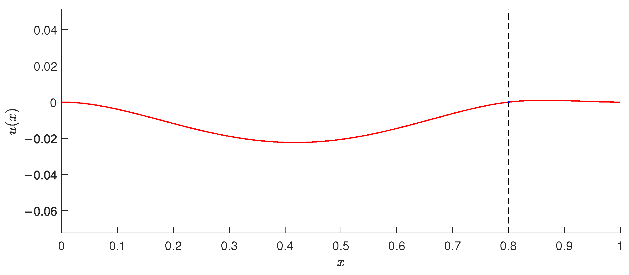
To provide a specific set of data for benchmark, we examine algorithms on the example of a steel beam (E = 2.15 × 10 11 Nm 2 ) of the length l = 1 m. The point obstacle with given friction is given by x ^ = 8 / 10 m with friction values g 1 = 10 2 N and g 2 = 5 × 10 4 N. We suppose the load function f = 50,000 N. The beam has a rectangular cross section of height v = 0.02 m and width s = 0.02 m. The analytical solution of this problem is presented in Figure 4.
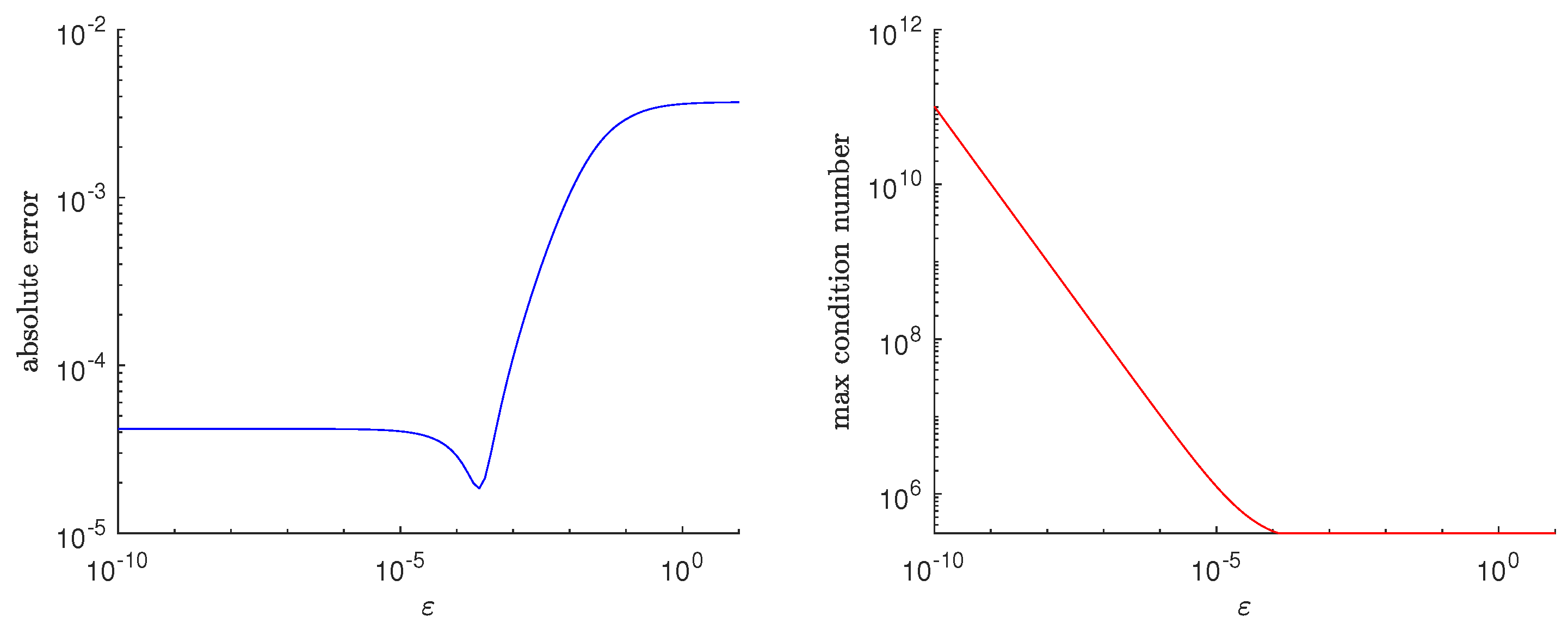
We start our examination with number of used elements as n = 20 and analyze the influence of regularization parameter on absolute error of the solution of regularized problem. We introduce the error measure by
err = 1 n + 1 i n + 1 u ¯ ( x i ) u ε * ( x i ) ,
where u ¯ is analytical solution and u ε * is numerical solution computed by solving (43) with regularization parameter ε . This formula measures the relative difference between the solutions in used nodal points. The results are presented in Figure 5.
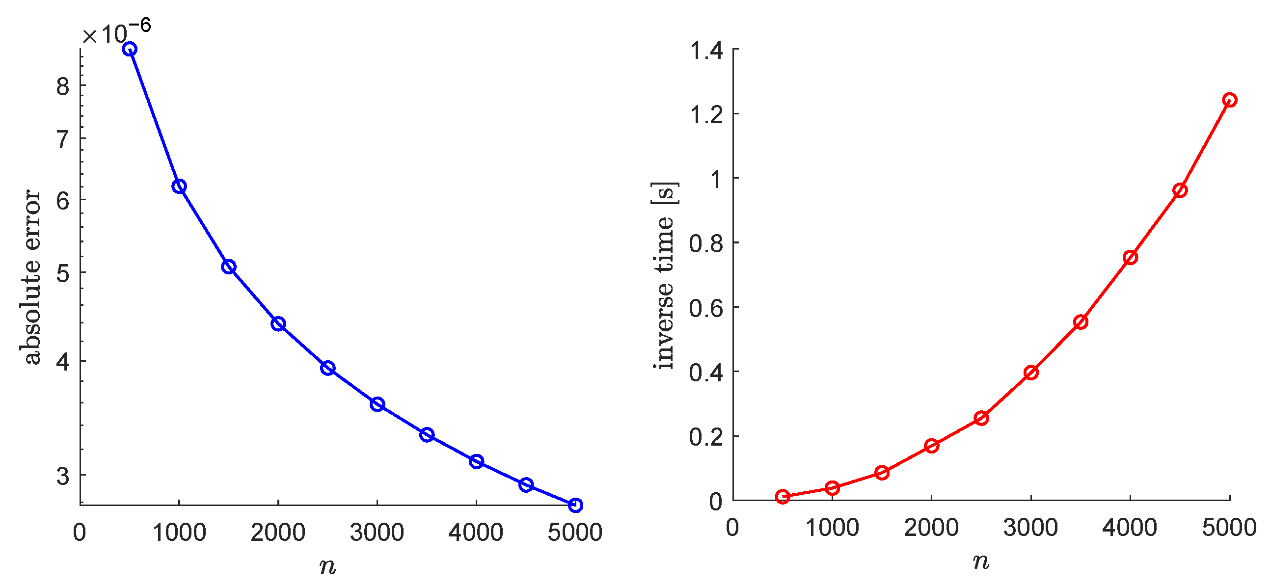
In the case of the dual problem, the absolute error decreases naturally with the increase of the discretization density, see Figure 6. The main bottleneck of this approach is the computation of the inverse.
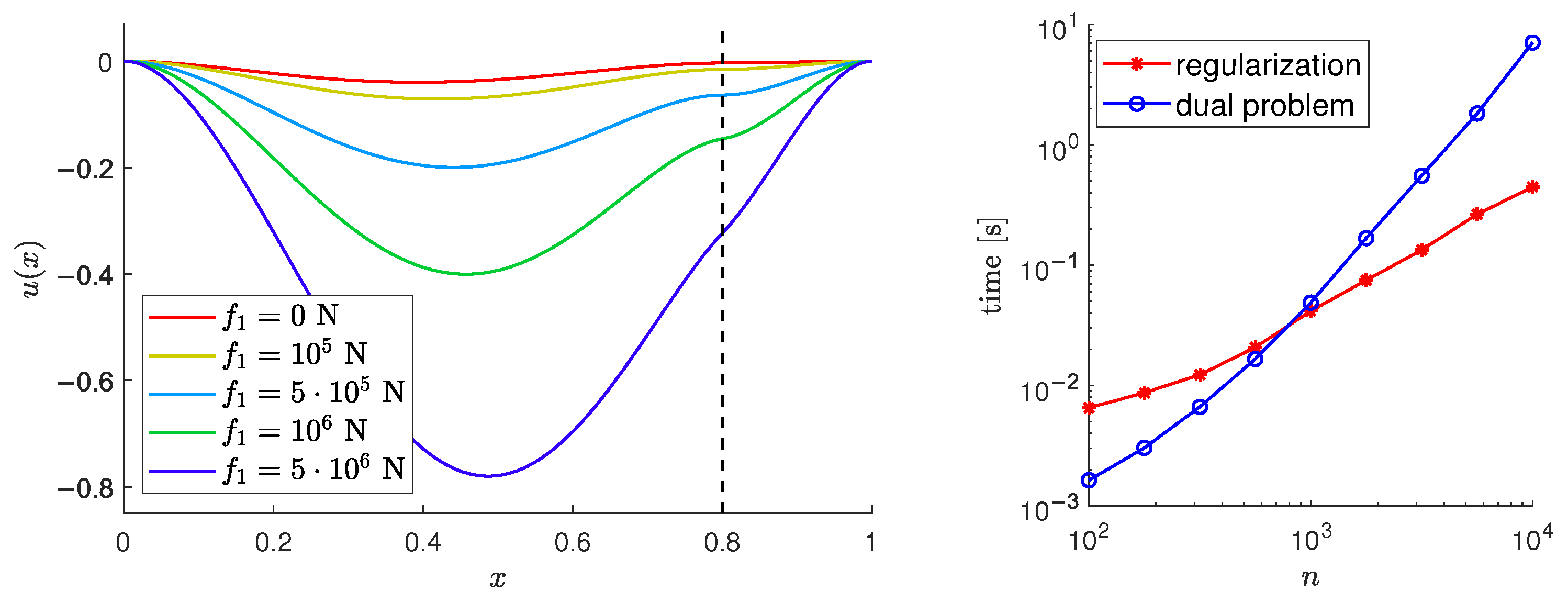
Benchmark 2
In this benchmark, we consider the same problem parameters as in the case of Benchmark 1 except for a shape of cross section and a load function. We consider a solid circular cross section of radius r = 0.01 m and a load function
f ( x ) = f 0 + ( f 1 f 0 ) x
with given parameters f 0 , f 1 R . Obviously, f is a linear function with f ( 0 ) = f 0 and f ( l ) = f ( 1 ) = f 1 .
Computing the corresponding integrals, it is easy to derive the components of a vector of right–hand sides
b 2 i = h 3 15 ( f 1 f 0 ) , b 2 i 1 = h ( f 0 + i h ( f 1 f 0 ) ) , i = 1 , , n .
We set f 0 = 10 5 N and solve the problem for various choice of f 1 , see Figure 7 (left). To compare the regularization method and the dual problem method, we solve the problem with f 1 = 1.5 × 10 5 N for increasing the problem dimension n. The computational time is demonstrated in Figure 7 (right). To decrease the small oscillations of the results (especially in the case of short time), we compute all problems 100 times and present the average computational time.
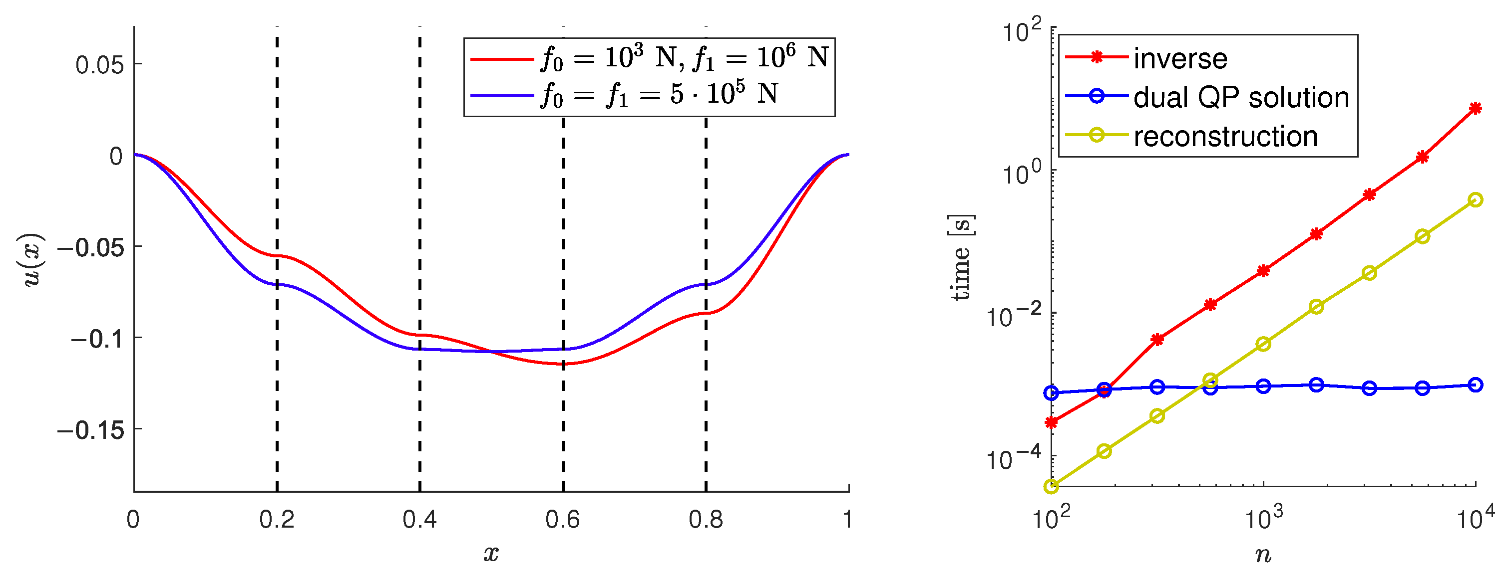
Benchmark 3
In our last benchmark, we increase the number of internal point obstacles with given friction coefficients to 4 equidistantly distributed on [ 0 , 1 ] . We consider the coefficients of given sliding and swivel friction the same for all points g 1 = 10 4 N and g 2 = 5 × 10 4 N. We consider material constants defined in Benchmark 1 and the solid circular cross section and load function defined in Benchmark 2. The solution provided by the dual problem approach is presented in Figure 8 (left). In the case of 4 obstacle points, the number of corresponding Lagrange multipliers λ is 8, g = [ g 1 , g 2 , g 1 , g 2 , g 1 , g 2 , g 1 , g 2 ] T R 8 and matrix B (45) has 8 rows. The dimension of dual problem (49) is 8; however, the most time-consuming operation remains the inverse of the Hessian matrix, see Figure 8 (right).

3. Discussion

For the demonstration, we plot the largest condition number from nine systems, which has to be solved, see Figure 5. The exact source of the problem is the term 1 / ε added to diagonal elements of the Hessian matrix of corresponding regularized problem, see Table 1 for exact equations.
Figure 5 demonstrates the typical problem with regularization: the decrease of regularization parameter decreases the error of solution; however, it consequently increases the condition number of the system matrix A ^ . The additional term from the gradient of approximated function (Table 1) is shifting some of the diagonal values of the original SPD matrix A . Using the Gershgorin circle theorem [20], we can state that with decreasing ε , the corresponding centers of Gershgorin discs (which includes eigenvalues) are converging to infinity, keeping the radius of disks (sum of absolute values of non-diagonal elements in the corresponding row) constant. Consequently, some of the eigenvalues are converging to infinity. As other eigenvalues remain unchanged, the condition number of the modified matrix A ^ is converging to infinity. The system becomes ill-conditioned.
The speed of convergence of iterative numerical algorithms for solving SPD systems (e.g., Conjugate Gradient method [18]) depends crucially on condition number. On the other hand, if we decide to solve the problem using the direct method (e.g., Gauss elimination method), we hit the finite limits of arithmetical operation. To be more specific, at some point in the process, we have to divide by large number on a diagonal. We can conclude that with decreasing ε , it is harder to solve the system precisely.
On the other hand, the dual algorithm is not using any regularization, and therefore it is not necessary to tune this parameter to obtain the optimal ratio between the condition number of the corresponding matrix and the error of approximation. However, this approach has a big price: the assembly of the dual problem. In dual problem (49), one has to compute the inverse of the Hessian matrix, which typically scales with O ( n 3 ) . In our benchmarks, the Hessian matrix is sparse with a suitable structure to obtain scaling O ( n 2 ) , see results from Benchmark 1 presented in Figure 6 (right), as well as solution of Benchmark 3 presented in Figure 8 (right). In comparison to the regularization method, the computation of inverse is at some point the bottleneck of the dual problem approach, and the method is slower than the regularization approach, see Figure 7 (right). It is necessary to mention that there exist techniques to avoid the computation of the inverse, e.g., the factorization or the matrix-free implementation [21]. Additionally, the reconstruction of primal solution from dual solution (48) can be performed as a solution of a system of linear equations instead of the multiplication with a dense inverse matrix. This is the reason why (using our naive implementation) the reconstruction step scales with O ( n 2 ) in Figure 8.
It is necessary to highlight that we did not solve Benchmark 3 with the regularization method. For multiple obstacle points, the number of corresponding equations (43) would be equal to the number of all combinations of Table 1 constructed for each obstacle point. This number scales exponentially with the number of obstacle nodes. For instance, in the case of 4 points, we would have to solve 9 4 systems of linear equations (43). On the other hand, the dual problem is a much more efficient approach: increasing the number of obstacle points increases the size of the dual problem linearly.

4. Conclusions

In this paper, we presented both the theoretical and practical aspects of solving the bending problem of the beam: starting from variational formulation, discussing the discretization by Finite Element Method, and ending with numerical methods for solving the corresponding optimization problem. Our numerical experiments revealed the advantages and disadvantages of the two most basic techniques for dealing with the non-differentiable friction term in objective function: the regularization method and the dual problem approach.
The performance and efficiency of the regularization method depend on the a priori chosen parameter. If this parameter is large, the approximation of the original function is not sufficient, and consequently the solution of the approximated problem can be wrong. If the parameter is small, the corresponding problem is ill-conditioned and hard to solve. Additionally, in the case of the problem with more obstacle points, this approach becomes practically inapplicable.
The method of dual problem transforms the problem onto the problem of Lagrange multipliers. The size of the problem is equal to the number of defined friction conditions in the original problem. However, the transformation requires the computation with the inverse of the Hessian matrix of the original problem.
Nevertheless, the explicit computation of the inverse matrix can be avoided using smart implementation techniques. This will be the topic of our future research.

Author Contributions

Conceptualization, M.B.; methodology, M.B. and L.P.; software, L.P.; validation, M.B. and L.P.; formal analysis, M.B.; investigation, M.B.; resources, M.B. and L.P.; data curation, M.B.; writing—original draft preparation, M.B.; writing—review and editing, M.B. and L.P.; visualization, M.B. and L.P.; supervision, M.B.; project administration, L.P.; funding acquisition, L.P. All authors have read and agreed to the published version of the manuscript.

Funding

This paper has been completed thanks to the financial support provided to VSB-Technical University of Ostrava by the Czech Ministry of Education, Youth and Sports from the budget for conceptual development of science, research and innovations for the 2021 year.

Institutional Review Board Statement

Not applicable.

Informed Consent Statement

Not applicable.

Data Availability Statement

In the case of the interest in Matlab implementation used in the paper, please contact the corresponding author.

Acknowledgments

Authors would like to express grateful thanks to the Department of Mathematics for comments, motivation, and the creative environment full of support.

Conflicts of Interest

The authors declare no conflict of interest.

Appendix A

Throughout the paper, we used the following notation:
  • D = d d x ;
  • u ( x ) -deflection of the beam;
  • u V -norm u in space V;
  • E ( x ) -Young’s modulus of elasticity of material ( 0 < E 0 E ( x ) );
  • J ( x ) -moment of inertia of the cross-section ( 0 < J 0 J ( x ) );
  • M ( u ( x ) ) -bending moment at the point x ( 0 , l ) , where
    M ( u ( x ) ) = E ( x ) J ( x ) D 2 u ( x ) ,
    M ( u ( x ¯ ) ) = lim x x ¯ M ( u ( x ) ) ,
    M ( u ( x ¯ ) ) = lim x x ¯ + M ( u ( x ) ) ;
  • T ( u ( x ) ) -shear force at the point x ( 0 , l ) , where
    T ( u ( x ) ) = D ( M ( u ( x ) ) ) = D ( E ( x ) J ( x ) D 2 u ( x ) ) ,
    T ( u ( x ¯ ) ) = lim x x ¯ T ( u ( x ) ) ,
    T + ( u ( x ¯ ) ) = lim x x ¯ + T ( u ( x ) ) ;
  • V * -dual space of V;
  • ( u , v ) -scalar product in L 2 ( ( 0 , l ) ) .

References

  1. Janečka, A.; Pruša, V.; Rajagopal, K.R. Euler–Bernoulli type beam theory for elastic bodies with nonlinear response in the small strain range. Arch. Mech. 2016, 68, 3–25. [Google Scholar]
  2. Yang, G.D. Nonlinear elastic beam theory with application in contact problems and variational approaches. Mech. Res. Commun. 1996, 23, 11–17. [Google Scholar] [CrossRef]
  3. Machalova, J.; Netuka, H. Solution of Contact Problems for Nonlinear Gao Beam and Obstacle. J. Appl. Math. 2015, 2015, 12. [Google Scholar] [CrossRef] [Green Version]
  4. Ahn, J.; Stewart, D.E. An Euler–Bernoulli Beam with Dynamic Frictionless Contact: Penalty Approximation and Existence. Numer. Funct. Anal. Optim. 2007, 28, 1003–1026. [Google Scholar] [CrossRef]
  5. Zhu, X.; Li, L. A well-posed Euler-Bernoulli beam model incorporating nonlocality and surface energy effect. Appl. Math. Mech. Engl. Ed. 2019, 40, 1561–1588. [Google Scholar] [CrossRef]
  6. Machalová, J.; Netuka, H. Optimal control of system governed by the Gao beam equation. Conf. Publ. 2015, 2015, 783. [Google Scholar] [CrossRef]
  7. Rektorys, K. Variational Methods in Mathematics, Science and Engineering; Science and Engineering; Springer: Berlin/Heidelberg, Germany, 2001. [Google Scholar]
  8. Hlaváček, I.; Haslinger, J.; Nečas, J.; Lovíšek, J. Solution of Variational Inequalities in Mechanics; Springer: Berlin/Heidelberg, Germany, 1988. [Google Scholar]
  9. Ekeland, I.; Téman, R. Convex Analysis and Variational Problems; SIAM: Philadelphia, PA, USA, 1999. [Google Scholar]
  10. Reddy, J. An Introduction to Finite Element Method, 3rd ed.; McGraw-Hill: New York, NY, USA, 2006. [Google Scholar] [CrossRef] [Green Version]
  11. Trémolières, R.; Lions, J.; Glowinski, R. Numerical Analysis of Variational Inequalities; North–Holand: Amsterdam, The Netherlands, 1981. [Google Scholar]
  12. Dostál, Z. Optimal Quadratic Programming Algorithms, with Applications to Variational Inequalities; SOIA; Springer: New York, NY, USA, 2009; Volume 23. [Google Scholar]
  13. Fucik, S.; Kufner, A. Nonlinear Differential Equations; Elsevier: Amsterdam, The Netherlands, 1980. [Google Scholar]
  14. Aubin, J.P. Approximation of Elliptic Boundary-Value Problems; Willey-Interscience: London, UK, 1972. [Google Scholar]
  15. Lions, J.L.; Stampacchia, G. Variational inequalities. Commun. Pure Appl. Math. 1967, 20, 493–519. [Google Scholar] [CrossRef] [Green Version]
  16. Ciarlet, P.G. The Finite Element Method for Elliptic Problems; North–Holand: Amsterdam, The Netherlands, 1979. [Google Scholar]
  17. Tibshirani, R. Regression Shrinkage and Selection via the Lasso. J. R. Stat. Soc. Ser. B 1996, 58, 267–288. [Google Scholar] [CrossRef]
  18. Nocedal, J.; Wright, S.J. Numerical Optimization, 2nd ed.; Springer: New York, NY, USA, 2006. [Google Scholar]
  19. Pospíšil, L.; Bobková, M. The Dual Formulation of Discretized Beam Bending Problem with Sliding and Swivel Friction. In Proceedings of the ICNAAM Conference, AIP Conference Proceedings, Rhodes, Greece, 17–23 September 2020. [Google Scholar]
  20. Golub, G.H.; Loan, C.F.V. Matrix Computations, 4th ed.; Johns Hopkins University Press: Baltimore, MD, USA, 2013. [Google Scholar]
  21. Horák, D.; Hapla, V.; Kružík, J.; Sojka, R.; Čermák, M.; Tomčala, J.; Pecha, M.; Dostál, Z. A Note on Massively Parallel Implementation of FETI for the Solution of Contact Problems. Adv. Electr. Electron. Eng. 2017, 15. [Google Scholar] [CrossRef]
Figure 1. Fixed beam with internal point obstacle with given swivel and sliding friction.
Mathematics 09 00898 g001
Figure 2. Cubic polynomials used as finite element basis for the problem discretization.
Mathematics 09 00898 g002
Figure 3. The approximation of absolute value by differentiable function.
Mathematics 09 00898 g003
Figure 4. (Benchmark 1): The analytical solution.
Mathematics 09 00898 g004
Figure 5. (Benchmark 1): The influence of the regularization parameter on absolute error (left) and the maximum condition number of 9 systems of linear equations have to be solved during the process (right).
Mathematics 09 00898 g005
Figure 6. (Benchmark 1): The problem of the dual formulation is the computational cost of the assembly of the objects. The most time-consuming operation is the computation of inverse (right). However, the decrease in the error with increasing density of discretization is an indisputable advantage (left).
Mathematics 09 00898 g006
Figure 7. (Benchmark 2): The solution for various choices of load function parameters (left) and the computational time for the selected problem (right). The measured time is an average from 100 runs of the algorithm.
Mathematics 09 00898 g007
Figure 8. (Benchmark 3): The solution for two different choices of load function parameters solved by the dual problem method (left) and the computational time of operations performed during the solution process for the selected problem (right). The inverse denotes the computation of Hessian inverse, the dual QP solution is a solution of (49), and the reconstruction is an evaluation of (48). The measured time is an average from 100 runs of the algorithm.
Mathematics 09 00898 g008
Table 1. The non-zero components of gradient of the approximated non-differentiable term in the objective function.
c 2 j ^ 1
( , ε ) [ ε , ε ] ( ε , )
c 2 j ^ ( , ε ) [ q ˜ N , ε ( c ) ] 2 j ^ 1 = g 1 [ q ˜ N , ε ( c ) ] 2 j ^ 1 = g 1 ε c 2 j ^ 1 [ q ˜ N , ε ( c ) ] 2 j ^ 1 = g 1
[ q ˜ N , ε ( c ) ] 2 j ^ = g 2 [ q ˜ N , ε ( c ) ] 2 j ^ = g 2 [ q ˜ N , ε ( c ) ] 2 j ^ = g 2
[ ε , ε ] [ q ˜ N , ε ( c ) ] 2 j ^ 1 = g 1 [ q ˜ N , ε ( c ) ] 2 j ^ 1 = g 1 ε c 2 j ^ 1 [ q ˜ N , ε ( c ) ] 2 j ^ 1 = g 1
[ q ˜ N , ε ( c ) ] 2 j ^ = g 2 ε c 2 j ^ [ q ˜ N , ε ( c ) ] 2 j ^ = g 2 ε c 2 j ^ [ q ˜ N , ε ( c ) ] 2 j ^ = g 2 ε c 2 j ^
( ε , ) [ q ˜ N , ε ( c ) ] 2 j ^ 1 = g 1 [ q ˜ N , ε ( c ) ] 2 j ^ 1 = g 1 ε c 2 j ^ 1 [ q ˜ N , ε ( c ) ] 2 j ^ 1 = g 1
[ q ˜ N , ε ( c ) ] 2 j ^ = g 2 [ q ˜ N , ε ( c ) ] 2 j ^ = g 2 [ q ˜ N , ε ( c ) ] 2 j ^ = g 2
Publisher’s Note: MDPI stays neutral with regard to jurisdictional claims in published maps and institutional affiliations.

