Impact of Regional Difference in Recovery Rate on the Total Population of Infected for a Diffusive SIS Model

Abstract

This paper is concerned with an SIS epidemic reaction-diffusion model. The purpose of this paper is to derive some effects of the spatial heterogeneity of the recovery rate on the total population of infected and the reproduction number. The proof is based on an application of our previous result on the unboundedness of the ratio of the species to the resource for a diffusive logistic equation. Our pure mathematical result can be epidemically interpreted as that a regional difference in the recovery rate can make the infected population grow in the case when the reproduction number is slightly larger than one.

1. Introduction

Because of the spread of COVID-19, the role of mathematical models in infectious disease epidemiology is becoming more important. This paper is aim to assert that, by mathematical analysis for a diffusive SIS model, a regional difference of recovery rates of infectious disease can make the total population of infected become large. In the field of reaction–diffusion equations, the following SIS model has been studied since thre paper by Allen, Bolker, Lou, and Nevai [1]:

$$\left\{\begin{array}{cc}{\displaystyle \frac{\partial S}{\partial t}}=d_S\Delta S-\beta \left(x\right){\displaystyle \frac{SI}{S+I}}+\gamma \left(x\right)I,\hfill & (x\in \mathsf{\Omega },t>0),\hfill \\ {\displaystyle \frac{\partial I}{\partial t}}=d_I\Delta I+\beta \left(x\right){\displaystyle \frac{SI}{S+I}}-\gamma \left(x\right)I,\hfill & (x\in \mathsf{\Omega },t>0),\hfill \\ {\displaystyle \frac{\partial S}{\partial \nu }}={\displaystyle \frac{\partial I}{\partial \nu }}=0,\hfill & (x\in \partial \mathsf{\Omega },t>0),\hfill \\ S(x,0)=S_0\left(x\right)\ge 0,I(x,0)=I_0\left(x\right)\ge (\not\equiv )0\hfill & (x\in \mathsf{\Omega }),\hfill \end{array}\right.$$

(1)

where $\mathsf{\Omega }$ is a bounded domain in ${\mathbb{R}}^n$ with smooth boundary $\partial \mathsf{\Omega }$; $\Delta :={\sum }_{j=1}^n{\partial }^2/\partial x_j^2$ is the Laplace operator and $\partial /\partial \nu$ is the directional derivative in the direction of the outward unit normal vector $\nu$. This epidemic model describes the spatio-temporal dynamics of the population densities of susceptible and infected. The unknown functions $S(x,t)$ and $I(x,t)$ stand for the population densities of susceptible and infected at location $x=(x_1,\dots ,x_n)$ in the habitat $\mathsf{\Omega }$ and time $t>0$, respectively. Given non-negative piecewise smooth functions $\beta \left(x\right)$ and $\gamma \left(x\right)$, respectively, indicate the rates of disease transmission and recovery from infection. The given positive constants $d_S$ and $d_I$ represent the random diffusion rates of susceptible and infected, respectively. The no-flux conditions on susceptible and infected are assumed.

The time-global well-posedness of (1) is known, as follows (see e.g., [2]): For each non-negative initial data $(S_0,I_0)\in L^{\infty }\left(\mathsf{\Omega }\right)\times L^{\infty }\left(\mathsf{\Omega }\right)$ with $\parallel I_0{\parallel }_{L^1}:={\int }_{\mathsf{\Omega }}{I}_0\left(x\right)dx>0$, there exists a unique positive solution $(S,I)\in C^{1+\theta ,(1+\theta )/2}(\overline{\mathsf{\Omega }}\times (0,\infty ))\times C^{1+\theta ,(1+\theta )/2}(\overline{\mathsf{\Omega }}\times (0,\infty ))$ for any $\theta \in (0,1)$ and, moreover, $(S,I)$ satisfies the mass conservation law:

$${\int }_{\mathsf{\Omega }}(S(x,t)+I(x,t))dx={\int }_{\mathsf{\Omega }}(S_0\left(x\right)+I_0\left(x\right))dx=:N\mathrm{for}\mathrm{any}t>0,$$

(2)

that is to say, the model (1) assumes a spatio-temporal scale, in which the total population of susceptible and infected is conserved. It is conjectured that any solution $(S,I)$ of (1) tends to a non-negative stationary solution as $t\to \infty$. Therefore, in order to know the spatial distribution of susceptible and infected after a long time, it is important to study the steady-state problem, as follows:

$$\left\{\begin{array}{cc}{d}_s\Delta S+\beta \left(x\right){\displaystyle \frac{SI}{S+I}}-\gamma \left(x\right)I=0,S\ge 0\hfill & (x\in \mathsf{\Omega }),\hfill \\ d_I\Delta I-\beta \left(x\right){\displaystyle \frac{SI}{S+I}}+\gamma \left(x\right)I=0,I\ge 0\hfill & (x\in \mathsf{\Omega }),\hfill \\ {\displaystyle \frac{\partial S}{\partial \nu }}={\displaystyle \frac{\partial I}{\partial \nu }}=0,\hfill & (x\in \partial \mathsf{\Omega }),\hfill \\ {\displaystyle {\int }_{\mathsf{\Omega }}(S+I)dx=N.}\hfill \end{array}\right.$$

(3)

Corresponding to the disease free situation, (3) with $I=0$ admits a unique solution

$$(S,I)=\left({\displaystyle \frac{N}{\left|\mathsf{\Omega }\right|}},0\right),$$

(4)

which is called the disease free equilibrium (DFE). On the other hand, a solution $(S,I)$ of (3) with $S>0$ and $I>0$ in $\mathsf{\Omega }$ is called an endemic equilibrium (EE). In [1], it was shown that the reproduction number ${\mathcal{R}}_0$ (will be introduced in the next section) plays a threshold for the existence/nonexistence of EE in the sense that there is no EE if ${\mathcal{R}}_0\le 1$, whereas there is a unique EE if ${\mathcal{R}}_0>1$. In the field of reaction–diffusion equations, the singular limit of EE as $d_S$ or $d_I$ tends to zero has been studied by [1,3,4,5]. Concerning related research works on (1) or (3), we refer to [6,7,8,9,10,11,12,13,14,15,16,17,18,19] and the references therein.

The purpose of this paper is to show a tendency that some concentration profile of $\beta \left(x\right)-\gamma \left(x\right)$ in the equal diffusion case $d_S=d_I$ makes ${\parallel I\parallel }_{L^1}$ grow. To be precise, it will be shown that, under the same level of ${\mathcal{R}}_0^{\infty }:={\parallel \beta \parallel }_{L^1}/{\parallel \gamma \parallel }_{L^1}>1$, the total population of infected in a heterogeneous setting of $\beta \left(x\right)-\gamma \left(x\right)$ is larger than that in the homogeneous setting of $\beta \left(x\right)-\gamma \left(x\right)$. For instance, if the transmission rate $\beta \left(x\right)$ is uniform over $\mathsf{\Omega }$ and the recovery rate $\gamma \left(x\right)$ is very poor within a small area of $\mathsf{\Omega }$, then the total population of infected will be higher than that in the case of the uniform transmission and recovery rates over $\mathsf{\Omega }$ with the same level of ${\mathcal{R}}_0^{\infty }$. That is to say, the regional difference of the recovery rate can make the total population of infected grow.

The proof is an application of our result [20] on the profile of the positive stationary solution to a diffusive logistic equation. In [20], the authors proved that some spatial concentration setting of a resource function in the diffusive logistic equation makes the $L^1$ norm of the positive stationary solution become as large as possible. It will be shown that, in the case of $d_S=d_I$, (3) can be reduced to a single equation, which is similar to the stationary diffusive logistic equation. By a change of variable, the growth property of the total population of infected will be related to the growth property of $L^1$ norm of the stationary solutions to the logistic equation.

This paper is organized, as follows: in Section 2, the known results on (1) and (3) and our result on the diffusive logistic equation will be introduced. In Section 3, the main result on the growth property of the total population of infected will be proved. Furthermore, some pure and numerical analysis of the reproduction number will be shown. In Section 4, some related issues to the results of this paper will be presented.

2. Known Results

2.1. Diffusive SIS Model

In this subsection, we introduce the known results on the SIS model (1) and the associated stationary problem (3). Concerning the long-time behavior of solutions of (1), Allen et al. [1] proved that the following reproduction number ${\mathcal{R}}_0$ plays an important threshold in the sense of Theorem 1,

$${\mathcal{R}}_0(d_I;\beta ,\gamma ):=\underset{\phi \in H^1\left(\mathsf{\Omega }\right)\backslash \left\{0\right\}}{sup}{\displaystyle \frac{{\int }_{\mathsf{\Omega }}\beta \left(x\right){\phi }^{2}dx}{d_I{\parallel \nabla \phi \parallel }_2^2+{\int }_{\mathsf{\Omega }}\gamma \left(x\right){\phi }^{2}dx}}.$$

(5)

It is noted that ${\mathcal{R}}_0$ is characterized as the principal eigenvalue of the following eigenvalue problem

$$\left\{\begin{array}{cc}{d}_I\Delta \phi +\left(\frac{\beta \left(x\right)}{\lambda }-\gamma \left(x\right)\right)\phi =0\hfill & (x\in \mathsf{\Omega }),\hfill \\ \frac{\partial \phi }{\partial \nu }=0\hfill & (x\in \partial \mathsf{\Omega }).\hfill \end{array}\right.$$

(6)

Here, it is noted that (6) has infinitely many eigenvalues $\left\{{\lambda }_j\right\}$ that are all real and ${\mathcal{R}}_0$ is the maximum eigenvalue.

Theorem 1

([1]). The reproduction number ${\mathcal{R}}_0(d_I;\beta ,\gamma )$ is monotone decreasing with respect to $d_I>0$, and it satisfies

$$\underset{d_I\to +0}{lim}{\mathcal{R}}_0(d_I;\beta ,\gamma )=\underset{x\in \overline{\mathsf{\Omega }}}{sup}\frac{\beta \left(x\right)}{\gamma \left(x\right)},\underset{d_I\to \infty }{lim}{\mathcal{R}}_0(d_I;\beta ,\gamma )=\frac{{\parallel \beta \parallel }_{L^1}}{{\parallel \gamma \parallel }_{L^1}}(={\mathcal{R}}_0^{\infty }).$$

(7)

Furthermore, the following (i) and (ii) hold true:

(i) 

If $0<{\mathcal{R}}_0<1$, then DFE (obtained by (4)) is globally asymptotically stable (GAS) in the sense that all solutions of (1) tend to DFE uniformly in $\overline{\mathsf{\Omega }}$ as $t\to \infty$, and, moreover, there is no EE.

(ii) 

If ${\mathcal{R}}_0>1$, then DFE is unstable, and, moreover, there exists a unique EE.

It is conjectured that the unique EE is globally asymptotically stable when ${\mathcal{R}}_0>1$. In some special cases, the validity was proved by [18,19]. As mentioned in Introduction, since the pioneering work [1], (1) and (3) have been studied by a lot of researchers in the field of reaction–diffusion equations from various viewpoints.

2.2. Diffusive Logistic Equation

In this subsection, we introduce known results on a diffusive logistic equation in the bounded domain $\mathsf{\Omega }$ of ${\mathbb{R}}^n$. The results will be related to our analysis for the profile of solutions of (3). We consider the following diffusive logistic equation:

$$\left\{\begin{array}{cc}{\displaystyle \frac{\partial u}{\partial t}}=d\Delta u+u(m\left(x\right)-u),\hfill & (x\in \mathsf{\Omega },t>0),\hfill \\ {\displaystyle \frac{\partial u}{\partial \nu }}=0,\hfill & (x\in \mathsf{\Omega },t>0),\hfill \\ u(x,0)=u_0\left(x\right)\ge \not\equiv 0,\hfill & (x\in \mathsf{\Omega }),\hfill \end{array}\right.$$

(8)

where the unknown function $u(x,t)$ represents the population density of the species at location $x\in \mathsf{\Omega }$ and time $t>0$, a positive coefficient d is the random diffusion rate of the species, and $m\left(x\right)$ is called a resource function that stands for the density of resource (feed) for the species. This paper will assume a class of $m\left(x\right)$, as follows:

$$m\in L_{+}^{\infty }\left(\mathsf{\Omega }\right):=\{m\in L^{\infty }\left(\mathsf{\Omega }\right)\mid m\left(x\right)\ge 0\mathrm{a}.\mathrm{e}.x\in {\mathsf{\Omega },\parallel m\parallel }_{L^{\infty }}>0\}.$$

It is well-known that (8) admits a unique time-global solution $u\in C^{1+\theta ,(1+\theta )/2}(\overline{\mathsf{\Omega }}\times (0,\infty ))$ if $u_0\in L_{+}^{\infty }\left(\mathsf{\Omega }\right)$ and u tends to a unique positive solution to the following steady-state problem, as $t\to \infty$:

$$\left\{\begin{array}{cc}d\Delta u+u\left(m\right(x)-u)=0,u\ge 0,\hfill & (x\in \mathsf{\Omega }),\hfill \\ {\displaystyle \frac{\partial u}{\partial \nu }}=0,\hfill & (x\in \mathsf{\Omega }),\hfill \end{array}\right.$$

(9)

More precisely, the following result is well-known:

Theorem 2

([21]). For any $d>0$ and $m\in L_{+}^{\infty }\left(\mathsf{\Omega }\right)$, (9) admits a unique positive solution $u_{d,m}\in W^{2,p}\left(\mathsf{\Omega }\right)$ for any $p>1$. If $u_0\in L_{+}^{\infty }\left(\mathsf{\Omega }\right)$, then the solution of $u(x.t)$ of (8) satisfies ${lim}_{t\to \infty }u(·,t)=u_{d,m}$ uniformly in $\overline{\mathsf{\Omega }}$. That is to say, $u_{d,m}$ is globally asymptotically stable (GAS).

In the sense of Theorem 2, it is important to study the profile of $u_{d,m}$ in order to know the final spatial distribution of the species after a long time. From such a view-point, Ni proposed the following optimization problem: Find the value of

$$S_n:=\underset{d>0,m\in L_{+}^{\infty }\left(\mathsf{\Omega }\right)}{sup}{\displaystyle \frac{\parallel u_{d,m}{\parallel }_{L^1}}{{\parallel m\parallel }_{L^1}}}.$$

(10)

Hence, ${\parallel m\parallel }_{L^1}$ and $\parallel u_{d,m}{\parallel }_{L^1}$ represent the total amount of resource and the total population of the final state of the species, respectively. Subsequently, the variational problem (10) can be ecologically interpreted as “How much can the species survive per unit resource?” As a trigger to consider the problem (10), Lou [22] exhibited a fundamental, but unusual, procedure for (9), as follows: Multiplying $1/u_{d,m}$ by (9) and integrating the resulting expression over $\mathsf{\Omega }$ yields

$$d{\int }_{\mathsf{\Omega }}{\displaystyle \frac{\Delta u_{d,m}}{u_{d,m}}}dx+{\parallel m\parallel }_{L^1}-{\parallel u_{d,m}\parallel }_{L^1}=0.$$

Here, the integration by parts and the boundary condition leads to

$${\int }_{\mathsf{\Omega }}{\displaystyle \frac{\Delta u_{d,m}}{u_{d,m}}}dx={\int }_{\mathsf{\Omega }}{\left({\displaystyle \frac{|\nabla u_{d,m}|}{u_{d,m}}}\right)}^{2}dx\ge 0.$$

Subsequently, one can see that, for any $d>0$ and $m\in L_{+}^{\infty }\left(\mathsf{\Omega }\right)$, $\parallel u_{d,m}{\parallel }_{L^1}/{\parallel m\parallel }_{L^1}\ge 1$, where the equality only holds when $m\left(x\right)$ is constant. That is to say, a heterogeneity of $m\left(x\right)$ can make the total population of the species grow. It follows that $S_n>1$ for any dimension number n. In the research field of diffusive logistic equations, there was a conjecture that $S_n$ is finite for any n, and, especially, $S_1=3$ (see [23,24]). Bai, He, and Li shows the validity of $S_1=3$ [25].

However, in [20], the authors proved $S_n=\infty$ in the higher-dimensional case when $\mathsf{\Omega }$ is a unit ball $B_1^n:=\{x\in {\mathbb{R}}^n\mid \left|x\right|<1\}$ and $n\ge 2$. This is a big contrast to the one-dimensional case [25], where the supremum is 3. The proof is based on the sub-super solution method, employing a concentration setting of resources near the center as

$$m_{\epsilon }\left(x\right):=\left\{\begin{array}{cc}1/{\epsilon }^n\hfill & (x\in \overline{B_{\epsilon }^n}:=\{x\in {\mathbb{R}}^n\mid \left|x\right|\le \epsilon \left\}\right),\hfill \\ 0\hfill & (x\in \overline{B_1^n}\backslash \overline{B_{\epsilon }^n}).\hfill \end{array}\right.$$

Afterwards, a control of the diffusion rate as $d_{\epsilon }=O(1/{\epsilon }^{n-2})$ enables us to construct an $L^1$ unbounded sequence of sub-solutions as $\epsilon \to 0$.

Theorem 3

([20]). Suppose that the dimension number n satisfies $n\ge 2$. If $c_1>0$ and $c_2>0$ satisfy

$$1-2c_{1}n(n-1)-c_2\ge 0\mathrm{and}2c_{1}n-\frac{c_2}{e}\ge 0,$$

(11)

then the unique positive solution $u_{\epsilon }\left(x\right)$ of

$$\left\{\begin{array}{cc}\frac{c_1}{{\epsilon }^{n-2}}\Delta u+u(m_{\epsilon }\left(x\right)-u)=0\hfill & x\in B_1^n,\hfill \\ \frac{\partial u}{\partial \nu }=0\hfill & x\in \partial B_1^n.\hfill \end{array}\right.$$

satisfies

$$u_{\epsilon }\left(x\right)\ge \left\{\begin{array}{cc}\frac{c_2}{{\epsilon }^n}{e}^{-{\left|x\right|}^n/{\epsilon }^n}\hfill & (x\in \overline{B_{\epsilon }^n}),\hfill \\ \frac{c_2}{{e\left|x\right|}^n}\hfill & (x\in \overline{B_1^n}\backslash \overline{B_{\epsilon }^n})\hfill \end{array}\right.$$

(12)

for any $0<\epsilon <1$.

It is noted that (11) forms a triangle whose vertices are

$$(c_1,c_2)=(0,0),\left(\frac{1}{2n(e+n-1)},\frac{e}{e+n-1}\right),\left(\frac{1}{2n(n-1)},0\right).$$

on $(c_1,c_2)$ plane. By integrating the right-hand side of (12), one can see that the following inequality holds ([20], Theorem 2.2):

$$\frac{\parallel u_{\epsilon }{\parallel }_{L^1\left(B_1^n\right)}}{\parallel m_{\epsilon }{\parallel }_{L^1\left(B_1^n\right)}}\ge c_2\left(1-\frac{1}{e}+\frac{n}{e}|log\epsilon |\right)\mathrm{for}\epsilon \in (0,1).$$

Setting $\epsilon \to +0$ in this estimate, we obtain $S_n=\infty$ if $n\ge 2$. From the ecological viewpoint, this result implies that the total population of the species grows larger and larger, regardless of the limited total resources when the support of resources shrinks ($\epsilon \to 0$).

3. Main Results and Proofs

3.1. Profiles of the Infected Population Density

In order to apply Theorem 3 to the $L^1$ estimate of EE, in what follows we consider (3) with the following three conditions:

$$\mathsf{\Omega }=B_1^2(=:B_1)\left(\mathrm{unit}\mathrm{disk}\right)$$

and

$$d_S=d_I(=:d)\left(\mathrm{equal}\mathrm{diffusion}\right)$$

and

$$\beta \left(x\right)\equiv \overline{\beta }:=2/{\epsilon }^2,\gamma \left(x\right)=\tilde{\gamma }\left(x\right):=\left\{\begin{array}{cc}1/{\epsilon }^2\hfill & \mathrm{for}x\in \overline{B_{\epsilon }},\hfill \\ 2/{\epsilon }^2\hfill & \mathrm{for}x\in \overline{B_1}\backslash \overline{B_{\epsilon }}.\hfill \end{array}\right.$$

(13)

Hereafter, $B_r^2$ will be denoted by $B_r$ for simplicity. This setting (13) assumes a situation where the rate of disease transmission is uniform, but the recovery rate is poor within the centered area $B_{\epsilon }$.

Because of the equal diffusion setting, it is natural to introduce a new unknown function

$$w\left(x\right):=S\left(x\right)+I\left(x\right).$$

Subsequently, (3) is equivalent to

$$\left\{\begin{array}{cc}d\Delta w=0,w\ge 0\hfill & (x\in B_1),\hfill \\ d\Delta I+I(\beta -\gamma -\frac{\beta }{w}=1),I\ge 0\hfill & (x\in B_1),\hfill \\ {\displaystyle \frac{\partial w}{\partial \nu }}={\displaystyle \frac{\partial I}{\partial \nu }}=0,\hfill & (x\in \partial B_1),\hfill \\ {\displaystyle {\int }_{\mathsf{\Omega }}wdx=N.}\hfill & \end{array}\right.$$

(14)

Obviously, we have

$$w\left(x\right)\equiv \overline{w}:=\frac{N}{|B_1|}=\frac{N}{\pi }.$$

Thus, if we obtain the profiles of $I\left(x\right)$, we also know $S\left(x\right)=\overline{w}-I\left(x\right)$. By the setting of

$$m\left(x\right):=\overline{\beta }-\tilde{\gamma }\left(x\right)\mathrm{and}v\left(x\right):=\frac{\overline{\beta }}{\overline{w}}I\left(x\right),$$

the function $v\left(x\right)$ satisfies the diffusive logistic Equation (9). Subsequently, we can apply the results in [20] to $v\left(x\right)\left(I\right(x\left)\right)$. Here, we define a positive constant

$$\overline{\gamma }:={\int }_{B_1}\tilde{\gamma }dx=\pi \left(\frac{2}{{\epsilon }^2}-1\right)$$

(15)

so that levels of ${\mathcal{R}}_0^{\infty }$ are the same as $\parallel \overline{\beta }{\parallel }_{L^1}/\parallel \tilde{\gamma }{\parallel }_{L^1}=\parallel \overline{\beta }{\parallel }_{L^1}/{\parallel \overline{\gamma }\parallel }_{L^1}$. Our main theorem in this subsection is stated, as follows.

Theorem 4.

Let $\tilde{I}\left(x\right)$ be the solution to (14) with the heterogeneous recovery rate $\gamma \left(x\right)$ defined in (13), and $\overline{I}\left(x\right)$ be the solution to (14) with the homogeneous $\gamma \left(x\right)$ that is defined in (15). Subsequently, there exists a constant α, such that for any $\epsilon \in (0,1)$, the following inequality holds:

$$\frac{\parallel \tilde{I}{\parallel }_{L^1}}{\parallel \overline{I}{\parallel }_{L^1}}\ge \alpha \left(1-\frac{1}{e}+\frac{2}{e}|log\epsilon |\right).$$

Proof. 

Thanks to the change of variables $v\left(x\right)=(\overline{\beta }/\overline{w})I\left(x\right)$ and Theorem 3, we choose $\alpha =c_2$, then

$$\tilde{I}\left(x\right)\ge \left\{\begin{array}{cc}\frac{\alpha \overline{w}}{2}{e}^{-{\left|x\right|}^2/{\epsilon }^2}\hfill & (x\in \overline{B_{\epsilon }}),\hfill \\ \frac{\alpha \overline{w}{\epsilon }^2}{{2e\left|x\right|}^2}\hfill & (x\in \overline{B_1}\backslash \overline{B_{\epsilon }}).\hfill \end{array}\right.$$

Therefore, we obtain the following lower estimate:

$$\parallel \tilde{I}{\parallel }_{L^1}\ge \frac{\alpha \pi {\epsilon }^2\overline{w}}{2}\left(1-\frac{1}{e}+\frac{2}{e}|log\epsilon |\right).$$

On the other hand, in the homogeneous recovery situation, it is easy to see that

$$\overline{I}\left(x\right)\equiv \overline{w}\left(1-\frac{\overline{\gamma }}{\overline{\beta }}\right)=\frac{{\epsilon }^2\overline{w}}{2}.\mathrm{Hence},{\parallel \overline{I}\left(x\right)\parallel }_{L^1}=\frac{\pi {\epsilon }^2\overline{w}}{2}.$$

These imply the required assertion. □

This theorem states that, under the same level of ${\mathcal{R}}_0^{\infty }={\parallel \beta \parallel }_{L^1}/{\parallel \gamma \parallel }_{L^1}$, the total population of infected in a heterogeneous setting of $m\left(x\right)=\beta \left(x\right)-\gamma \left(x\right)$ is larger than that in the homogeneous setting of $m\left(x\right)$. This mathematical result can be interpreted as that if the disease transmission rate $\beta \left(x\right)$ is uniform over $B_1$ and the recovery rate $\gamma \left(x\right)$ is low within a small centered area of $B_1$, then the total population of infected in the heterogeneous setting grows larger than that in the homogeneous setting. That is to say, the regional difference of the rate of recovery can make the total population of infected grow with the order $O\left(\right|log\epsilon \left|\right)$ as $\epsilon \to 0$.

3.2. Analysis of the Reproduction Number

In this subsection, we assume that $\beta$ and $\gamma$ are defined by (13). In order to obtain radial solutions of the eigenvalue problem (6), we consider the following boundary value problem:

$$\left\{\begin{array}{cc}{\phi }_{rr}+\frac{1}{r}{\phi }_r+\frac{1}{d}\left(\frac{\overline{\beta }}{\lambda }-\tilde{\gamma }\left(r\right)\right)\phi =0\hfill & (0<r<1),\hfill \\ {\phi }_r\left(0\right)={\phi }_r\left(1\right)=0.\hfill \end{array}\right.$$

(16)

We recall that the maximum eigenvalue of $\left\{{\lambda }_j\right\}$ is equal to ${\mathcal{R}}_0$. By the radial symmetry of $\phi \left(x\right)$ and $\tilde{\gamma }\left(x\right)$, we write $\phi \left(r\right)=\phi \left(x\right)$ and $\tilde{\gamma }\left(r\right)=\tilde{\gamma }\left(x\right)$ $(r=|x\left|\right)$ for simplicity. Concerning the range of ${\mathcal{R}}_0$, we obtain the following lemma:

Lemma 1.

For any $d>0$ and $\epsilon \in (0,1)$, it holds that $1<{\mathcal{R}}_0(d,\epsilon )<2$.

Proof. 

Let $\phi \left(r\right)$ be a positive eigenfunction that corresponds to the principal eigenvalue $\lambda ={\mathcal{R}}_0$. By the definition of the reproduction number (5), we can see that

$${\mathcal{R}}_0\ge \frac{{\int }_{B_1}\overline{\beta }dx}{0+{\int }_{B_1}\tilde{\gamma }dx}=\frac{1}{1-{\epsilon }^2/2}>1.$$

Suppose ${\mathcal{R}}_0\ge 2$ to derive a contradiction. Afterwards, by (13), we have the following inequality

$${\phi }_{rr}+\frac{1}{r}{\phi }_r=\frac{1}{d{\epsilon }^2}\left(1-\frac{2}{{\mathcal{R}}_0}\right)\phi \ge 0\mathrm{for}\mathrm{any}r\in (0,\epsilon ).$$

Multiplying the above equation by r and integrating over $(0,r)$, we obtain $r\phi \ge 0$ for $0\le r\le \epsilon$. Here, we used ${\phi }_r\left(0\right)=0$. Hence, we have

$$\phi (\epsilon -0):=\underset{r\nearrow \epsilon }{lim}\phi \left(r\right)\ge 0.$$

(17)

We also see

$${\phi }_{rr}+\frac{1}{r}{\phi }_r=\frac{2}{d{\epsilon }^2}\left(1-\frac{1}{{\mathcal{R}}_0}\right)\phi >0\mathrm{for}\mathrm{any}r\in (\epsilon ,1).$$

Hence, multiplying the above equation by r and integrating over $(r,1)$, we obtain

$$\phi (\epsilon +0):=\underset{r\searrow \epsilon }{lim}\phi \left(r\right)<0.$$

(18)

Here, we used ${\phi }_r\left(1\right)=0$. On the other hand, the eigenfunction $\phi$ is in $C^1$-class. This contradicts (17) and (18). Therefore, we obtain $1<{\mathcal{R}}_0<2$. □

By the profile of the step function $\tilde{\gamma }$, we divide the region $B_1$ into two regions; the low recovery region $B_{\epsilon }$ and the high recovery region $B_1\backslash B_{\epsilon }$. Afterwards, we consider the following two initial value problems in order to construct two parts of solutions of (16) over $B_{\epsilon }$ and $B_1\backslash B_{\epsilon }$:

$$\left\{\begin{array}{cc}{\phi }_{rr}+\frac{1}{r}{\phi }_r+\frac{A^2}{{\epsilon }^2}\phi =0\hfill & (0<r<\epsilon ),\hfill \\ {\phi }_r\left(0\right)=0\hfill \end{array}\right.$$

(19)

and

$$\left\{\begin{array}{cc}{\phi }_{rr}+\frac{1}{r}{\phi }_r-\frac{B^2}{{\epsilon }^2}\phi =0\hfill & (\epsilon <r<1),\hfill \\ {\phi }_r\left(1\right)=0,\hfill \end{array}\right.$$

(20)

where

$$A=A(d,\lambda ):=\sqrt{\frac{1}{d}\left(\frac{2}{\lambda }-1\right)}\mathrm{and}B=B(d,\lambda ):=\sqrt{\frac{2}{d}\left(1-\frac{1}{\lambda }\right)}(1<\lambda <2).$$

It is known that the solution of (19) is expressed by

$$\phi \left(r\right)=C{J}_0\left(\frac{A}{\epsilon }r\right)(C:\mathrm{arbitrary}\mathrm{constant}),$$

where $J_0\left(z\right)$ is the Bessel function of the first kind. On the other hand, the solution of (20) is expressed by

$$\phi \left(r\right)=D\left(I_0\left(\frac{B}{\epsilon }r\right)+\frac{I_1(B/\epsilon )}{K_1(B/\epsilon )}{K}_0\left(\frac{B}{\epsilon }r\right)\right)(D:\mathrm{arbitrary}\mathrm{constant}),$$

where $I_0\left(z\right),K_0\left(z\right)$ are the modified Bessel functions of the first and second kind, respectively.

To accomplish the construction of the solution of (16), we need to connect two solutions of (19) and (20) at $r=\epsilon$ in $C^1$-class. For this end, we consider the following algebraic equations

$$C{J}_0\left(A\right)=\phi \left(\epsilon \right)=D\left(I_0\left(B\right)+\frac{I_1(B/\epsilon )}{K_1(B/\epsilon )}{K}_0\left(B\right)\right)$$

and

$$-C\frac{A}{\epsilon }{J}_1\left(A\right)={\phi }_r\left(\epsilon \right)=D\frac{B}{\epsilon }\left(I_1\left(B\right)-\frac{I_1(B/\epsilon )}{K_1(B/\epsilon )}{K}_1\left(B\right)\right),$$

equivalently,

$$\left[\begin{array}{cc}{J}_0\left(A\right)& -\left(I_0\left(B\right)+\frac{I_1(B/\epsilon )}{K_1(B/\epsilon )}{K}_0\left(B\right)\right)\\ -A{J}_1\left(A\right)& -B\left(I_1\left(B\right)-\frac{I_1(B/\epsilon )}{K_1(B/\epsilon )}{K}_1\left(B\right)\right)\end{array}\right]\left[\begin{array}{c}C\\ D\end{array}\right]=\left[\begin{array}{c}0\\ 0\end{array}\right].$$

There exists a non-trivial solution $\phi \left(r\right)$ if and only if the determinant of the above coefficient matrix is zero, which is,

$$\left(B{J}_0\left(A\right)K_1\left(B\right)-A{J}_1\left(A\right)K_0\left(B\right)\right)\frac{I_1(B/\epsilon )}{K_1(B/\epsilon )}-B{J}_0\left(A\right)I_1\left(B\right)-A{J}_1\left(A\right)I_0\left(B\right)=0.$$

(21)

As a summary of this subsection, we obtain the following theorem.

Theorem 5.

Let β and γ be chosen by (13). For any $d>0$ and $\epsilon \in (0,1)$, the reproduction number ${\mathcal{R}}_0(d,\epsilon )$ (that is defined by the principal eigenvalue of (6)) is characterized by

$${\mathcal{R}}_0(d,\epsilon )=max\{\lambda \in (1,2)\mid \lambda satisfies\left(21\right)\}.$$

3.3. Numerical Simulation for the Reproduction Number

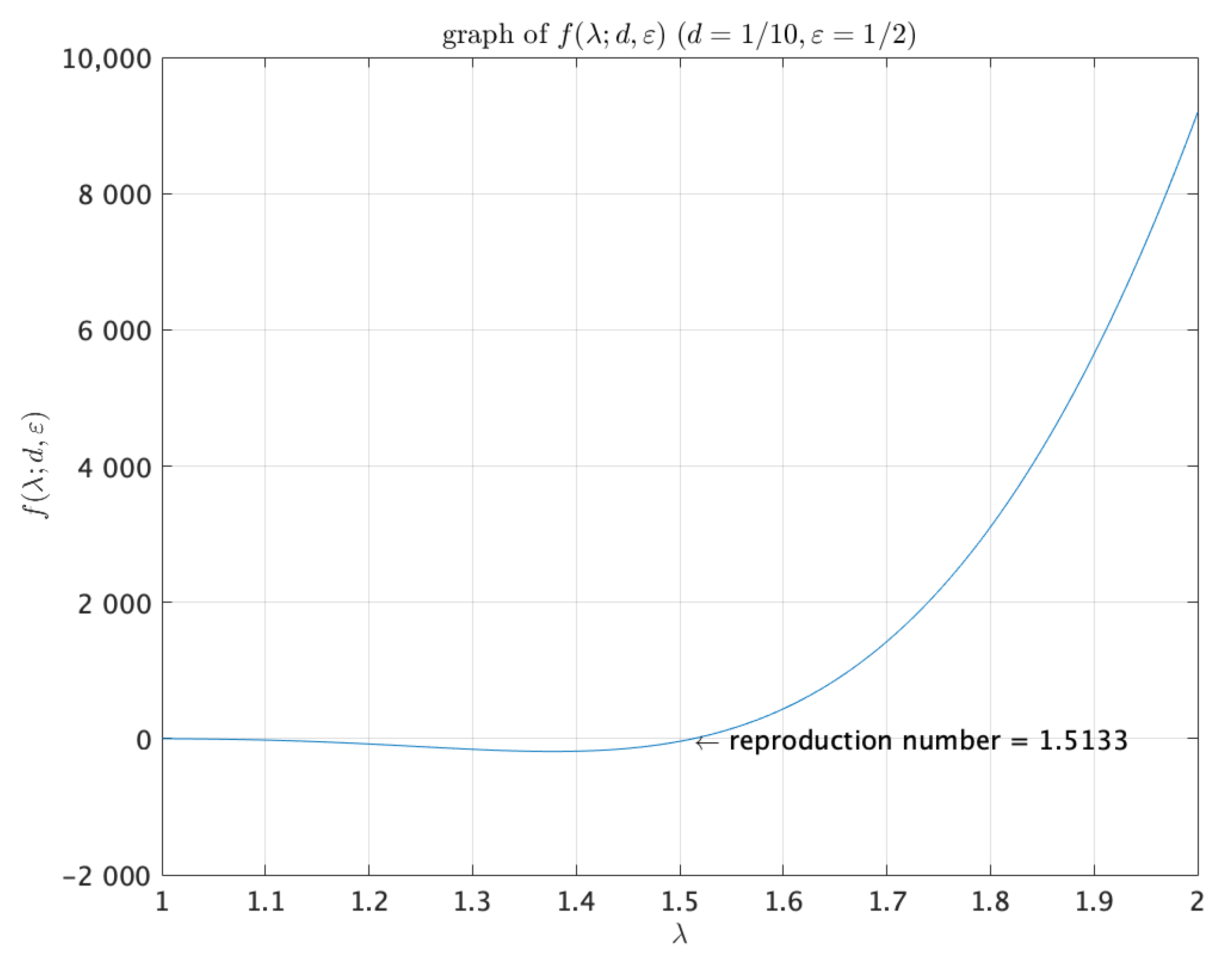
Based on Theorem 5, we show some numerical simulations of ${\mathcal{R}}_0$. We define the left-hand side of (21) by $f(\lambda ;d,\epsilon )$ for $\lambda \in (1,2),\epsilon \in (0,1)$ and $d>0$. Figure 1 shows the graph of $f\left(\lambda \right)$ in the case $d=1/10,\epsilon =1/2$. The setting of $\epsilon =1/2$ means that the disease transmission rate is a constant, which is, $\overline{\beta }\equiv 8$, but the recovery rate is non-constant:

$$\tilde{\gamma }\left(r\right)=\left\{\begin{array}{cc}4\hfill & (0<r<1/2),\hfill \\ 8\hfill & (1/2<r<1).\hfill \end{array}\right.$$

More precisely, in a unit-disk region, the value of the recovery rate is 4 within a half radius disk $B_{1/2}$; 8 outside the disk $B_{1/2}$. This setting realizes a situation that the recovery rate is equal to the disease transmission rate in the outer shell area $B_1\backslash B_{1/2}$, whereas the recovery rate is half the transmission rate in the central area $B_{1/2}$ and, so, the recovery rate is weaker than the transmission rate with respect to the average over the whole region $B_1$.

Figure 1. Graph of $f\left(\lambda \right)$ with $d=1/10$ and $\epsilon =1/2$.

We remark, from Theorem 5, that the graph of $f\left(\lambda \right)$ possesses infinitely many zero points, and each zero point corresponds to each eigenvalue of (16). The largest zero point of the graph is the reproduction number, in this case ${\mathcal{R}}_0=1.5133\cdots$.

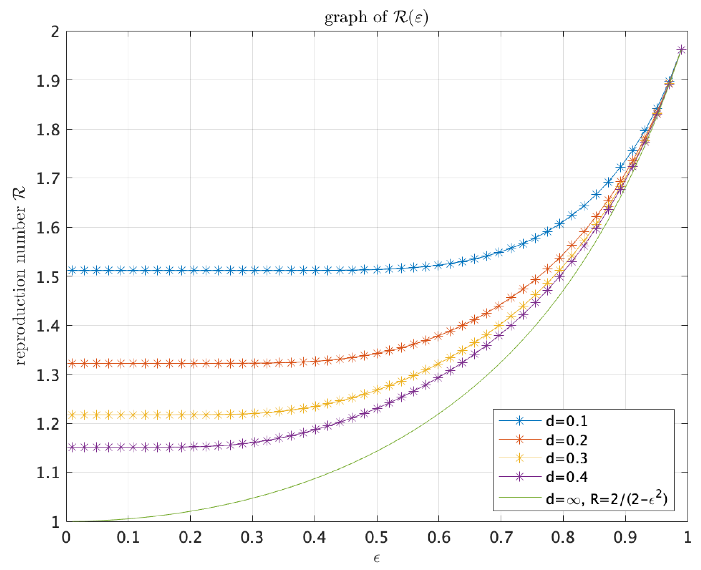
For fixed d, we have a map $(0,1)\ni \epsilon \mapsto {\mathcal{R}}_0\in (1,2)$, and so Figure 2 exhibits the $\epsilon$-dependence of the reproduction numbers ${\mathcal{R}}_0\left(\epsilon \right)$ for some d.

Figure 2. Graphs of ${\mathcal{R}}_0\left(\epsilon \right)$ for $d=0.1,0.2,0.3,0.4$, and ${\mathcal{R}}_0^{\infty }\left(\epsilon \right)=2/(2-{\epsilon }^2)$.

In Figure 2, the graph of ${\mathcal{R}}_0^{\infty }\left(\epsilon \right)=2/(2-{\epsilon }^2)$ represents ${\mathcal{R}}_0^{\infty }=\parallel \overline{\beta }{\parallel }_{L^1}/\parallel \tilde{\gamma }{\parallel }_{L^1}=\parallel \overline{\beta }{\parallel }_{L^1}/{\parallel \overline{\gamma }\parallel }_{L^1}$, which corresponds to the case ${lim}_{d\to \infty }{\mathcal{R}}_0$ from Theorem 1. We note that, for each $\epsilon \in (0,1)$, the reproduction number ${\mathcal{R}}_0$ is monotone decreasing with respect to d. Although this monotonicity has been proved in Theorem 1 mathematically, Figure 2 shows the concrete relationship between the reproduction number and the diffusion rate for fixed $\epsilon$. One can also observe that, for fixed some d, the reproduction number ${\mathcal{R}}_0$ is monotone increasing with respect to $\epsilon$. This monotone behavior can be epidemically interpreted as follows: First, we remember that $\epsilon \in (0,1)$ represents the level of heterogeneity of the recovery rate and also $\parallel \overline{\beta }{\parallel }_{L^1}/{\parallel \tilde{\gamma }\parallel }_{L^1}=2/(2-{\epsilon }^2)$ represents the ratio of the disease transmission rate to the recovery rate. In the extreme case when $\epsilon >0$ is very close to 0, then the ratio is about 1. On the other hand, if $\epsilon <1$ is very close to 1, then the ratio is about 2. Hence, the ratio $\parallel \overline{\beta }{\parallel }_{L^1}/{\parallel \tilde{\gamma }\parallel }_{L^1}$ makes the reproduction number be large. Finally, we can also see from Figure 2 that within the small $\epsilon$ range, the reproduction number with each fixed d is not much changed with respect to $\epsilon$, but the reproduction number with each fixed small $\epsilon >0$ drastically decreases as d increases; whereas within the range that $\epsilon$ is close to 1, the reproduction number with each fixed d drastically increases for $\epsilon$, but the reproduction numbers with various d are almost the same.

4. Discussion

In the previous section, we studied the impact of spatial heterogeneity of the recovery rate of individuals on the dynamics of an SIS epidemic reaction-diffusion model. Among other things, Theorem 4 asserts that the stationary infected population ${\parallel I\parallel }_{L^1}$ in the case of the heterogeneous recovery rate is larger than that in the case of homogeneous recovery rate. In this situation, the reproduction number ${\mathcal{R}}_0$ is larger than 1, but it is not so much larger. This means that, in the epidemic model sense, the scope of our analysis is in the small disease spread situation. Subsequently, it can be said that our result implies that, as long as the time-scale focusing on a pandemic sign period, the heterogeneity of the recovery rate can make the total infected population be worse in the sense that the ratio is large as $\parallel \tilde{I}{\parallel }_{L^1}/\parallel \overline{I}{\parallel }_{L^1}=O\left(\right|log\epsilon \left|\right)$ though both are still small as $\parallel \tilde{I}{\parallel }_{L^1}=O\left({\epsilon }^2\right)$ and $\parallel \overline{I}{\parallel }_{L^1}=O\left({\epsilon }^2\right)$.

Our analysis is also valid in the Kermack and McKendrick type SIS model (see [10]):

$$\left\{\begin{array}{cc}{S}_t=d_S\Delta S-\beta \left(x\right)SI+\gamma \left(x\right)I,\hfill & (x\in \mathsf{\Omega },t>0),\hfill \\ I_t=d_I\Delta I+\beta \left(x\right)SI-\gamma \left(x\right)I,\hfill & (x\in \mathsf{\Omega },t>0).\hfill \end{array}\right.$$

We assume the same diffusion rate $d:=d_S=d_I$ and put $w=S+I$, and then we obtain

$$\left\{\begin{array}{cc}{w}_t=d\Delta w,\hfill & (x\in \mathsf{\Omega },t>0),\hfill \\ I_t=d\Delta I+I(\beta \left(x\right)w-\gamma \left(x\right)-\beta \left(x\right)I),\hfill & (x\in \mathsf{\Omega },t>0).\hfill \end{array}\right.$$

when considering the stationary problem of the above model and the heterogeneous recovery rate $\gamma \left(x\right)$ setting, we can see the same result, which is, the spatial heterogeneity of $\gamma \left(x\right)$ makes the infected population grows larger than the homogeneous recovery rate setting.

References

- Allen, L.J.S.; Bolker, B.M.; Lou, Y.; Nevai, A.L. Asymptotic profiles of the steady states for an SIS epidemic reaction-diffusion model. Discret. Contin. Dyn. Syst. Ser. A 2008, 21, 1–20. [Google Scholar] [CrossRef]
- Ladyženskaja, O.A.; Solonnikov, V.A.; Ural’ceva, N.N. Linear and Quasi-Linear Equations of Parabolic Type; Translations of Mathematical Monographs, 23; ; American Mathematical Society: Providence, RI, USA, 1968. [Google Scholar]
- Peng, R. Asymptotic profiles of the positive steady state for an SIS epidemic reaction-diffusion model. I. J. Differ. Equ. 2009, 247, 1096–1119. [Google Scholar] [CrossRef]
- Peng, R.; Yi, F. Asymptotic profiles of the positive steady state for an SIS epidemic reaction-diffusion model: Effects of epidemic risk and population movement. Physica D 2013, 259, 8–25. [Google Scholar] [CrossRef]
- Wu, Y.; Zou, X. Asymptotic profiles of steady states for a diffusive SIS epidemic model with mass action infection mechanism. J. Differ. Equ. 2016, 261, 4424–4447. [Google Scholar] [CrossRef]
- Allen, L.J.S.; Bolker, B.M.; Lou, Y.; Nevai, A.L. Asymptotic profiles of the steady states for an SIS epidemic disease patch model. SIAM J. Appl. Math. 2007, 67, 1283–1309. [Google Scholar] [CrossRef]
- Cui, J.; Tao, X.; Zhu, H. An SIS infection model incorporating media coverage. Rocky Mount. J. Math. 2008, 38, 1323–1334. [Google Scholar] [CrossRef]
- Cui, R.; Lam, K.-Y.; Lou, Y. Dynamics and asymptotic profiles of steady states of an epidemic model in advective environments. J. Differ. Equ. 2017, 263, 2343–2373. [Google Scholar] [CrossRef]
- Cui, R.; Lou, Y. A spatial SIS model in advective heterogeneous environments. J. Differ. Equ. 2016, 261, 3305–3343. [Google Scholar] [CrossRef]
- Deng, K.; Wu, Y. Dynamics of a suscetible-infected-susceptible epidemic reaction-diffusion model. Proc. Roy. Soc. Edinb. Sect. A 2013, 146, 929–946. [Google Scholar] [CrossRef]
- Ding, W.; Huang, W.; Kansakar, S. Traveling wave solutions for a diffusive SIS epidemic model. Discret. Contin. Din. Syst. Ser. B 2013, 18, 1291–1304. [Google Scholar] [CrossRef]
- Gao, D.; Ruan, S. An SIS patich model with variable transmission coefficients. Math. Biosci. 2011, 232, 110–115. [Google Scholar] [CrossRef]
- Ge, J.; Kim, K.I.; Lin, Z.; Zhu, H. A SIS reaction-diffusion-advection model in a low-risk and high-risk domain. J. Differ. Equ. 2015, 259, 5486–5509. [Google Scholar] [CrossRef]
- Huang, W.; Han, M.; Liu, K. Dynamics of an SIS reaction-diffusion epidemic model for disease transmission. Math. Biosci. Eng. 2010, 7, 51–66. [Google Scholar]
- Kuto, K.; Matsuzawa, H.; Peng, R. Concentration profile of endemic equilibrium of a reaction-diffusion-advection SIS epidemic model. Calc. Var. Partial Differ. Equ. 2017, 56, 1–28. [Google Scholar] [CrossRef]
- Li, H.; Peng, R.; Wang, F.-B. Varying total population enhances disease persistence: Qualitative analysis on a diffusive SIS epidemic model. J. Differ. Equ. 2017, 262, 885–913. [Google Scholar] [CrossRef]
- Li, H.; Peng, R.; Xiang, T. Dynamics and asymptotic profiles of endemic equilibrium for two frequency-dependent SIS epidemic models with cross-diffusion. Eur. J. Appl. Math. 2020, 31, 26–56. [Google Scholar] [CrossRef]
- Peng, R.; Zhao, X.Q. A reaction-diffusion SIS epidemic model in a time-periodic environment. Nonlinearity 2012, 25, 1451–1471. [Google Scholar] [CrossRef]
- Peng, R.; Liu, S.Q. Global stability of the steady states of an SIS epidemic reaction-diffusion model. Nonlinear Anal. TMA 2009, 71, 239–247. [Google Scholar] [CrossRef]
- Inoue, J.; Kuto, K. On the unboundedness of the ratio of species and resources for the diffusive logistic equation. Discrete Contin. Dyn. Syst. Ser. B 2021, 26, 2441–2450. [Google Scholar] [CrossRef]
- Cantrell, R.S.; Cosner, C. Diffusive logistic equations with indefinite weights: Population models in disrupted environments. Proc. Roy. Soc. Edinb. Sect. A 1989, 112, 293–318. [Google Scholar] [CrossRef]
- Lou, Y. On the effects of migration and spatial heterogeneity on single and multiple species. J. Differ. Equ. 2006, 223, 400–426. [Google Scholar] [CrossRef]
- Lam, K.-L.; Lou, Y. Persistence, Competition and Evolution. In The Dynamics of Biological Systems; Bianchi, A., Hillen, T., Lewis, M., Yi, Y., Eds.; Springer: Berlin/Heidelberg, Germany, 2019; pp. 205–238. [Google Scholar]
- Lam, K.-L.; Liu, S.; Lou, Y. Selected topics on reaction-diffusion-advection models from spatial ecology. Math. Appl. Sci. Eng. 2020, 1, 150–180. [Google Scholar] [CrossRef]
- Bai, X.; He, X.; Li, F. An optimization problem and its application in population dynamics. Proc. Amer. Math. Soc. 2016, 144, 2161–2170. [Google Scholar] [CrossRef]
Publisher’s Note: MDPI stays neutral with regard to jurisdictional claims in published maps and institutional affiliations. |
© 2021 by the authors. Licensee MDPI, Basel, Switzerland. This article is an open access article distributed under the terms and conditions of the Creative Commons Attribution (CC BY) license (https://creativecommons.org/licenses/by/4.0/).