A Hybrid Strategic Oscillation with Path Relinking Algorithm for the Multiobjective k-Balanced Center Location Problem

Abstract

This paper presents a hybridization of Strategic Oscillation with Path Relinking to provide a set of high-quality nondominated solutions for the Multiobjective k-Balanced Center Location problem. The considered location problem seeks to locate k out of m facilities in order to serve n demand points, minimizing the maximum distance between any demand point and its closest facility while balancing the workload among the facilities. An extensive computational experimentation is carried out to compare the performance of our proposal, including the best method found in the state-of-the-art as well as traditional multiobjective evolutionary algorithms.

1. Introduction

Facility Location Problems (FLPs) are classical optimization problems that require finding the best placement to locate a set of facilities, which must serve a set of demand points. Note that the term best depends on the measure employed to model the FLP. The definition of this function is customized to the specific application, and it is typically set as a distance (or cost) function between demand points and facilities.

An FLP can be classified, in general terms, as discrete or continuous, weighted or unweighted, capacitated or incapacitated, and deterministic or stochastic according to the characteristics of the demand points and potential facilities. Additional elements can also be considered. Especially relevant is the inclusion of more than one objective function. As described in the review by Owen and Daskin [1], the necessity to use multiobjective modeling arises when a real-life problem is examined, for example, in locating obnoxious facilities. Current et al. [2] and Farahani et al. [3] provide comprehensive reviews of multiobjective discrete location problems.

Literature on FLP is vast, and we can find many different models depending on the elements in the previous classification. Some of the most popular are as follows:

-

Minimize the total (or average) distance (or cost) to service all demand points (k-Median problem, first studied by [4,5]);

-

Minimize the maximum distance from each demand point to its closest facility (k-Center problem, first solved by [6]);

-

Maximize the coverage provided by the facilities to demand points (Maximal Coverage location problem, first introduced in [7]);

-

Maximize the distance among all the facilities (k-Dispersion problem, see [8]);

-

Balance the distance among demand points and its closest facility, or even balance the number of demand points assigned to each facility (k-Balanced problem, see [9,10,11]).

In this paper, we target an important variant of FLP. Specifically, we consider a biobjective, discrete, unweighted, incapacitated, deterministic FLP, recently introduced in Davoodi [12]: the k-Balanced Center Location problem (k-BCL problem). The aim of the k-BCL problem is to locate k out of m facilities in order to serve a set of n demand points, with the aim of minimizing the maximum distance between each demand point and its closest selected facility (k-Center problem) while simultaneously balancing the number of demand points assigned to each selected facility (k-Balanced problem). The author studied the complexity of each formulation and concluded that the k-BCL problem is $\mathcal{NP}$-complete and, furthermore, he proposed an iterative algorithm based on the Voronoi diagram and Delaunay triangulation to solve the k-BCL problem, which is compared to a robust multiobjective evolutionary algorithm, the NSGA-II algorithm.

The goal of this paper is to propose a practical approach to solve the k-BCL problem. In particular, we propose an algorithm that uses the Greedy Randomized Adaptive Search Procedure (GRASP) to construct solutions [13] and then combines Strategic Oscillation (SO) [14,15] with Path Relinking (PR) [16] to further improve the set of efficient solutions found. The SO allows local search to oscillate between feasible and infeasible solutions to identify regions of the search space that are expected to contain better solutions. In order to repair the infeasible solutions, we apply a PR algorithm to explore the trajectories connecting pairs of solutions.

The rest of this paper is organized as follows. We first review facility location models related with the k-BCL problem in Section 2. In Section 3, we formally define this optimization problem; then, Section 4 describes the algorithms implemented to solve it (GRASP, SO, and PR). Section 5 presents the computational results performed to test the quality of the proposal, including a comparison with the previous approach. Finally, Section 6 draws some conclusions derived from the research and discusses future work.

2. Literature Review

This section is limited to review the facility location models somehow related to the k-BCL. We first review the literature addressing equity, and then the most recent papers on multiobjective facility location problems.

We can find many papers addressing equity in different ways. Finding an effective model is as important as balancing a subset of facilities, and depends on the nature of the real problem studied. Therefore, some models seek to guarantee the fairness in the distribution of costs or distance-to-travel among the demand points, and others emphasize equity from the facilities viewpoint. In the former idea, for example, we could highlight the works of Espejo et al. [17] and Berger and Bechwati [18]. In Espejo et al. [17], the authors proposed a discrete location problem where the equity is measured by the revealed preference of each demand point for the sites of the potential serving facilities; however, the aim of Berger and Bechwati [18] was to find the equity among the customers in the promotion budget allocation. Moreover, in the continuous framework, the equity question has been dealt with in different ways. For example, Drezner et al. [19] addressed it by minimizing the Gini index when a facility is located, while Berman and Kaplan [20] introduced a system of taxes that offset any inequalities that may arise due to travel costs. We should also mention the paper of Barbati and Bruno [21], where the authors reviewed the extensive literature about discrete facility location models that deal with the use of some equality measures of the distances between the facility and the demand points. Barbati and Piccolo [22] highlight that very often bicriteria optimization modeling is used to ensure a trade-off between the fairness and efficiency measures. This approach has been adopted by several authors such as Ogryczak [23], Ogryczak [24], Kostreva et al. [25], and more recently, Lejeune and Prasad [26] and Filippi et al. [27].

In this paper, we are interested in looking for equity from the facilities’ point of view. As described in Marín [11] and Davoodi [12], these models have applications in traffic networks [28] and Territory Design [29] such as locating schools, fire stations, or sport centers. This framework has been mostly ignored, and only in the last decade have a few specific models been proposed [11,12,30,31].

The work of Marín [11] deserves special attention. The author proposes the first discrete location model, where the number of demand points that are allocated to each facility is balanced. In particular, the problem entails establishing k facilities in such a way that the range between facilities with the most and least demand points assigned is minimized, and considering that each demand point is allocated to its closest facility. Marín [11] proposed two integer programming formulations, one of them comes from the k-Median problem, and the second one from the discrete ordered median problem [32]. Closely related to the previous study is the work of Daskin and Tucker [33], where the authors proposed a biobjective optimization problem to balance the median and range of the assigned demand.

The specific problem considered here, the k-Balanced Center Location (k-BCL) problem, was recently addressed in Davoodi [12], considering two different functions to measure the balance: minimize the maximum number of demand points assigned to each selected facility and minimize the difference between the maximum and minimum number of demand points assigned to each selected facility. To sum up,

Table 1. Classification of the references.

Location Space	Equity Viewpoint	References
Discrete, continuous	Theoretical	Erkut [9], Marsh and Schilling [10], Owen and Daskin [1], Current et al. [2], Farahani et al. [3], Barbati and Piccolo [22]
Continuous	Demand points	Berman and Kaplan [20], Drezner et al. [19]
Continuous	Facilities	Berman et al. [31], Kalcsics et al. [30]
Discrete	Demand points	Espejo et al. [17], Berger and Bechwati [18]
Discrete	Facilities	Marín [11], Daskin and Tucker [33], Davoodi [12]

shows the key publications in balanced facility location problems.

The majority of FLPs studied in the literature appear when a realistic situation must be solved. Usually, in those situations, decision makers propose locating facilities while considering more than one conflicting objective at a time and, therefore, forming a multiobjective optimization problem. For this reason, recently, the number of works related to multiobjective FLP have been considerably increasing. Next, some of the most recent and interesting papers are briefly mentioned but there exist many other variants depending on the objectives to optimize.

In 2017, different objectives were simultaneously considered in Karatas [34], where the coverage of the demand points is maximized while the total distance and the workload balancing of the facilities are minimized. One year later, in 2018, many different multiobjective FLPs were studied: Colmenar et al. [35] solved the biobjective obnoxious FLP, in which the objectives consist of maximizing the distances between each demand point and their nearest facility (obnoxious k-Median problem) and the dispersion among facilities (k-Dispersion problem).

We have identified several multiobjective variants of the k-Median problem. Wang et al. [36] considers the maximization of the total coverage provided by the selected facilities (the maximal coverage location problem) and, simultaneously, the minimization of the total distance (k-Median problem). The authors in Colmenar et al. [37] minimized the total distance among demand points and facilities (k-Median problem), and maximized the minimum distance between the selected facilities (k-Dispersion problem); Daskin and Tucker [33] solved a biobjective optimization problem by minimizing the total distance between each demand point and its closest facility (k-Median problem) and balancing the facility workload measured as the difference between the maximum and the minimum demand assigned to any facility. The same year, Karatas and Yakıcı [38] first proposed another multiobjective FLP in which three objectives are considered: the minimization of the maximum distance among demand points and facilities (k-Center problem), the minimization of the total distance among demand points and facilities (k-Median problem), and the maximization of the coverage provided by the selected facilities to demand points (the maximal coverage location problem); this same problem was also solved by López-Sánchez et al. [39] in 2020.

In 2019, Tutunchi and Fathi [40] and Pérez-Peló et al. [41] took into account two objectives: the minimization of the maximum distance among facilities and demand points (the k-Center problem), and the maximization of the minimum distance between all pairs of facilities (k-Dispersion problem).

After reviewing the papers above, we conclude that both equity and multiobjective are two key elements to model realistic location variants. However, they introduce additional complexity to models that are difficult by themselves. We therefore propose solving methods based on complex methodologies to target our realistic variant.

The main contributions of this work are as follows: (i) to propose a novel metaheuristic method to solve the k-BCL problem, (ii) to propose a new strategy based on PR to obtain feasible solutions when two infeasible solutions are combined, (iii) to propose a specific evaluation function, and (iv) to improve the state-of-the-art algorithms for solving the k-BCL problem.

3. The k-Balanced Center Location Problem

As described in the previous section, in this paper, we consider the k-BCL problem that, as far as we know, was first addressed by Davoodi [12] in 2019. The author summarized related works emphasizing that despite the long history of the k-center problem, facility location with the objective of maximum balance is a new problem and proposes different multiobjective formulations of the k-BCL problem that will be explained below.

The k-BCL problem can be defined as follows. Let $N=\{1,\dots ,n\}$ be a set of demand points and $M=\{1,\dots ,m\}$ be the set of candidate locations to host a facility. Let $d_{ij}$ be the distance between the demand point $i\in N$ and the facility $j\in M$. It is assumed that all demand points are serviced/assigned to their closest facility. We define $n_j$ as the number of demand points assigned to a facility j. The aim of the k-BCL problem is to locate a set of k out of m candidate facilities in order to minimize the maximum distance between each demand point and its closest selected facility, and balance the number of demand points assigned to each selected facility. More specifically, the former goal ensures that the distance traveled by each demand point is, at most, the obtained value, whereas the latter balances the number of demand points assigned to each selected facility—that is, to balance the workload of each selected facility.

Thus, Davoodi [12] formulates the k-BCL problem as a multiobjective facility location problem, where the first objective function is the one optimized in the k-Center problem, with the goal of obtaining a subset S of M with $\left|S\right|=k$ in such a way that

$$f_1\left(S\right)=\underset{i\in N}{max}\underset{j\in S}{min}{d}_{ij}$$

(1)

is minimized. Note that the considered problem forces that each demand point must be served by its closest facility.

In order to ensure a balanced solution, Davoodi [12] proposes two different functions to measure fairness among the facilities: the first one consists of minimizing the maximum number of demand points assigned to each facility, while the second one minimizes the difference between the maximum and minimum number of demand points served by any facility, which corresponds to the objective function of the Balanced Location Problem proposed by Marín [11]. Formally, they are respectively defined as minimizing the following two objective functions:    

$$\begin{array}{ccc}\hfill f_2\left(S\right)& =& \underset{j\in S}{max}{n}_j,\hfill \end{array}$$

(2)

$$\begin{array}{ccc}\hfill f_3\left(S\right)& =& \underset{j,j^{{}^{\prime }}\in S,j\ne j^{{}^{\prime }}}{max}\left|n_j-n_{j^{{}^{\prime }}}\right|.\hfill \end{array}$$

(3)

Following the notation by Davoodi [12], k-BLC${}_{12}$ is the biobjective optimization problem that arises when combining the objective functions $f_1\left(S\right)$ and $f_2\left(S\right)$. Similarly, k-BLC${}_{13}$ is the biobjective optimization problem that emerges when considering the objective functions $f_1\left(S\right)$ and $f_3\left(S\right)$. Finally, k-BLC${}_{123}$ is the multiobjective optimization problem that emerges when considering the objective functions $f_1\left(S\right)$, $f_2\left(S\right)$, and $f_3\left(S\right)$. The combination of functions $f_2\left(S\right)$ and $f_3\left(S\right)$ does not make sense since they are not in conflict. The three considered problems (k-BLC${}_{12}$, k-BLC${}_{13}$, and k-BLC${}_{123}$) in the Euclidean space are $\mathcal{NP}$-complete [12].

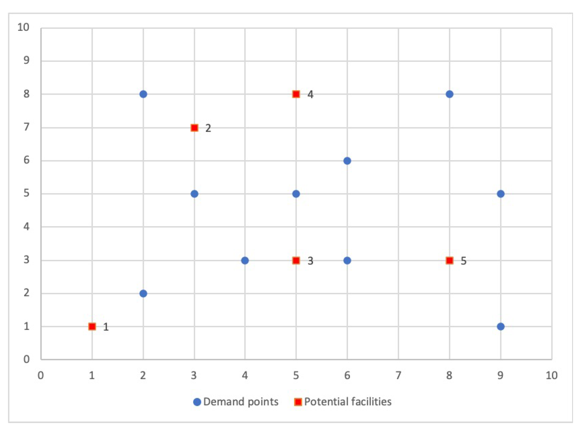
We would like to illustrate the advantages of a multiobjective approach with a simple example. Let us consider an instance of $n=10$ demand points (blue circles) and $m=5$ candidate facilities (red squares), shown in Figure 1, and we compute the distances between the demand points and the facilities by using the Euclidean metric.

The aim in this example is to locate $k=3$ facilities. We generate all the feasible solutions and compute, for each solution, the three objective functions. In 

Table 2. All feasible solutions.

S	${\mathit{n}}_{\mathit{S}}$	${\mathit{f}}_1\left(\mathit{S}\right)$	${\mathit{f}}_2\left(\mathit{S}\right)$	${\mathit{f}}_3\left(\mathit{S}\right)$
$\{1,2,3\}$	$(1,4,5)$	5.10	5	4
$\{1,2,4\}$	$(3,4,3)$	8.00	4	1
$\{1,2,5\}$	$(2,4,4)$	5.00	4	2
$\{1,3,4\}$	$(1,6,3)$	4.47	6	5
$\{1,3,5\}$	$(1,6,3)$	5.83	6	5
$\{1,4,5\}$	$(2,5,3)$	3.61	5	3
$\{2,3,4\}$	$(2,6,2)$	4.47	6	4
$\{2,3,5\}$	$(3,4,3)$	5.00	4	1
$\{2,4,5\}$	$(4,2,4)$	5.10	4	2
$\{3,4,5\}$	$(5,3,2)$	3.16	5	3

, we enumerate all of them (column S), then, we show the number of demand points assigned to its selected facility (column $n_S$) and the three objective function values ($f_1\left(S\right)$, $f_2\left(S\right)$, $f_3\left(S\right)$).

The best objective function values for each problem isolated are highlighted in bold font.

The data in Table 2 indicates that the optimal solution value for the first objective function is 3.16 units and the facilities must be located in plants 3, 4, and 5. However, the optimal solution for the second and third objective functions are 4 and 1, respectively. In fact, these values are reached simultaneously in solutions $\{1,2,4\}$ and $\{2,3,5\}$, however, $\{2,3,5\}$ exhibits better objective function value $f_1\left(S\right)$ than $\{1,2,4\}$. It is important to recall that functions $f_2\left(S\right)$ and $f_3\left(S\right)$ control the workload equity among the facilities and $f_1\left(S\right)$ handles the maximum distance between demand points and facilities. So, we realize that the solutions $\{2,3,5\}$ and $\{3,4,5\}$ are incomparable since solution $\{2,3,5\}$ is better regarding the second and third objective functions and solution $\{3,4,5\}$ is preferable concerning the first one. In conclusion, both goals are in conflict, as it is impossible to improve one of them without deteriorating the other.

Actually, as is widely known, the solution of a multiobjective problem is given by a set of efficient points (also called Pareto-optimal solutions), with the property that they cannot be improved simultaneously in all the objectives without necessarily worsening at least one of them [42]. In particular, in the example above, the Pareto-optimal set consists of the solutions $\{2,3,5\}$ and $\{3,4,5\}$.

Formally, we define the k-BLC as the multiobjective optimization problem

$$\underset{S\in \Omega }{min}F\left(S\right)={[f_1\left(S\right),f_2\left(S\right),f_3\left(S\right)]}^T,$$

where $\Omega$ is the set of all feasible solutions. Then, the Pareto-optimal set is formed by all nondominate solutions. In this context, given two solutions $S_1$ and $S_2$ in $\Omega$, we say that

• $S_1$ weakly dominates $S_2$, denoted as $S_1⪯S_2$, if and only if $F\left(S_1\right)\le F\left(S_2\right)$;
• $S_1$ dominates $S_2$, denoted as $S_1\prec S_2$, if and only if $S_1⪯S_2$ and at least one objective function of $F\left(S_1\right)$ is strictly better than the corresponding one of $F\left(S_2\right)$;
• $S_1$ strictly dominates $S_2$, denoted as $S_1⪯⪯S_2$, if and only if $F\left(S_1\right)<F\left(S_2\right)$.

In conclusion, the goal of multiobjective optimization is to find the Pareto-optimal set. We should bear in mind that it contains all the solutions that are not dominated by any member of the solution set. The image of the Pareto set is named the Pareto front. To obtain the Pareto front of the k-BCL problem, we will propose a metaheuristic able to obtain a good approximation of it with high-quality solutions in order to improve the state-of-the-art algorithms.

4. A Hybrid Strategic Oscillation with Path Relinking Algorithm

This section describes in detail the algorithm implemented to solve the k-BCL problem. We propose a methodology based on Strategic Oscillation (SO), which is a metaheuristic initially designed with the purpose of crossing back and forth between the feasible and infeasible solution spaces of an optimization problem. A feasible solution for the k-BCL problem is represented as a set S of k selected facilities to which demand points have been assigned. As previously mentioned, it is assumed that all demand points are assigned to its closest facility. Therefore, a solution is not feasible if the number of selected facilities is smaller or larger than k. To construct feasible and unfeasible solutions, a GRASP method has been implemented. Furthermore, we hybridize the SO algorithm with a combination method based on Path Relinking (PR) in order to improve the quality of the population found. Next, each of the phases of the proposed algorithm will be detailed step by step.

4.1. GRASP

The proposed SO algorithm requires an initial population of solutions to be processed. Although this initial set of solutions could be generated at random, any metaheuristic algorithm performs better, either in quality or in computing time, if the starting point is a population of high-quality solutions.

In order to do so, a Greedy Randomized Adaptive Search Procedure (GRASP) is used. GRASP algorithm is a well-known and widely used methodology to solve hard, combinatorial optimization problems. This algorithm, first proposed by Feo and Resende [43], is an iterative process, in which each iteration consists of two phases: a greedy randomized construction phase and a local search method. The former is designed for creating a solution from scratch, while the latter is designed to find a local optimum with respect to a certain neighborhood.

4.1.1. Construction Phase

As aforementioned, the construction phase is in charge of building a solution from scratch. The construction phase of a GRASP procedure has a distinguishing characteristic in the way that it combines greediness with randomness while a solution is being built. To that end, a solution is built by adding one element at each step using a greedy function $g\left(c\right)$ that measures the potential contribution of each candidate element, $c\in \mathit{CL}$, to the partial solution. This methodology considers a restricted candidate list, RCL, which contains a subset of the most promising elements to be included in the solution under construction, i.e., those elements whose incorporation into the partially built solution would yield the smallest increase according to the greedy function value, thus leading to a better solution. Specifically, $\mathit{RCL}=\{c\in \mathit{CL}:g\left(c\right)\le g_{min}+\alpha (g_{max}-g_{min})\}$, where $g_{min}$ and $g_{max}$ are the minimum and the maximum values of the greedy function of the elements in CL, respectively. The parameter $\alpha \in [0,1]$ determines the greediness of the method. On the one hand, if $\alpha =0$, the RCL contains only those elements whose greedy function value is the best one, i.e., $g\left(c\right)=g_{min}$, leading to a completely deterministic construction but for the ties. On the other hand, $\alpha =1$ implies constructing the RCL with all the candidate elements in CL, i.e., $g\left(c\right)=g_{max}$, which entails a completely random construction. Once the RCL have been constructed with the most promising elements, the next one to be included in the solution is then selected at random from it, updating the CL to reflect the fact that a new element has been added to the solution and is no longer available for selection. This greedy randomized selection of an element and update of the CL are repeated until a complete solution has been built. In this problem, the method iteratively adds elements until exactly k facilities have been added to the solution under construction.

To favor diversity, the proposed algorithm starts by selecting at random the first candidate element to be included in the partial solution under construction, as is customary in GRASP. Then, the remaining facilities $k-1$ are included in the partial solution under construction using a greedy function. In the context of the k-BCL problem, since we are dealing with a multiobjective optimization problem with three different objective functions, we propose using each one of them separately in every construction to generate solutions focused on every objective of the problem under consideration. These greedy functions are the three considered objective functions: $f_1\left(S\right)$, $f_2\left(S\right)$, or $f_3\left(S\right)$ (see functions (1), (2), or (3), respectively). The construction ends when k facilities has been selected, that is, $\left|S\right|=k$. Algorithm 1 shows the pseudocode for the GRASP construction used in this paper including all the details.

Our GRASP constructive procedure receives as input the demand points N, the candidate facilities M, the number of facilities to be selected k, the parameter that controls its greediness $\alpha$, and the set of efficient solutions ES. Initially, solution S is empty (step 1). Traditionally, GRASP selects the first facility at random from the set of candidate facilities M to diversify the search (step 2), including it as the initial facility of the solution under construction (step 3). Then, until k facilities are selected, the algorithm evaluates all the candidates facilities $v\in \mathit{CL}$ with a greedy function $g\left(v\right)$, storing the minimum (step 6) and maximum (step 7) values. Note that as we are solving a multiobjective problem, the greedy function will depend on the objective to be optimized, in our case, $f_1$, $f_2$, or $f_3$. In particular, in this work, a number of solutions are constructed for each objective separately (see Section 5 for specific details in this value). Then, the Restricted Candidate List, RCL, is computed by considering the value of the $\alpha$ parameter (step 8). The best value for this parameter must be deeply studied to reach a balance between greediness and randomness in the construction. Then, a facility is selected at random (step 9) from the RCL, updating the available candidate facilities CL (step 11). The function $\mathit{Insert}\&\mathit{Update}\left(S\right)$ checks if every obtained solution S is an efficient solution and, if so, it is inserted into the set of efficient solutions, denoted by $ES$, removing all solutions of the set that are dominated by S. The greedy algorithm ends by returning the set of efficient solutions (step 14).

Algorithm 1 GRASP(N, M, k, $\alpha$, ES)

1: $S\leftarrow \varnothing$ 2: $v\leftarrow \mathit{Random}\left(M\right)$ 3: $S\leftarrow S\cup \left\{v\right\}$ 4: $\mathit{CL}\leftarrow M\backslash \left\{v\right\}$ 5: while$\left|S\right|<k$do 6:     $g_{min}={min}_{v\in \mathit{CL}}g\left(v\right)$ 7:     $g_{max}={max}_{v\in \mathit{CK}}g\left(v\right)$ 8:     $\mathit{RCL}\leftarrow \{v\in \mathit{CL}:g\left(v\right)\le g_{\mathit{min}}+\alpha (g_{max}-g_{min})\}$ 9:     $u\leftarrow \mathit{Random}\left(RCL\right)$ 10:    $S\leftarrow S\cup \left\{u\right\}$ 11:    $\mathit{CL}\leftarrow \mathit{CL}\backslash \left\{u\right\}$ 12: end while 13:  $ES\leftarrow \mathit{Insert}\&\mathit{Update}\left(S\right)$ 14: return$ES$

4.1.2. Local Search Method

The second phase of the GRASP methodology consists explores the neighborhood of the solution given by the construction phase in order to find a local optimum. In single-objective optimization, a local search iteratively replaces the current solution with a better solution from its neighborhood. Nevertheless, in this work, we are dealing with multiobjective optimization problem, so here it is considered that a solution is better whenever the solution is a nondominated solution. The first requirement to define a local search method is the definition of the neighborhood to be explored. Given a solution S, the neighborhood $\mathcal{N}\left(S\right)$ is defined as the set of solutions that can be obtained by exchanging a selected facility with any nonselected facility. The exchange of a selected facility $u\in S$ with a nonselected one $v\in M\backslash S$ is formally defined as

$$\mathit{Exchange}(S,u,v)\leftarrow (S\backslash \{u\left\}\right)\cup \left\{v\right\}.$$

Then, the neighborhood considered in this work is defined as

$$\mathcal{N}\left(S\right)\leftarrow \left\{\mathit{Exchange}\right(S,u,v):u\in S,v\in M\backslash S\}.$$

Having defined the neighborhood to be explored, it is necessary to indicate how the neighborhood is explored and which moves are accepted. In the context of the k-BCL problem, we propose a first-improvement strategy, accepting the first move that leads to a nondominated solution, stopping when no new efficient solutions are found in the complete neighborhood.

Since this definition will lead to an exhaustive exploration of the solution space, which can eventually be slow, we propose a more sophisticated local search adapted to each objective function that we would like to optimize. To that end, we define the order in which the neighborhood is explored with the aim of first exploring the most promising solutions. Specifically, we propose two strategies, depending on if we are focusing on minimizing the distances between facilities and demand points, or in balancing the number of demand points assigned to each facility:

• ${\mathit{L}\mathit{S}}_{\mathit{m}}$: If we focus on minimizing the maximum distances between each demand point and its closest selected facility, the selected facilities are ordered from least to greatest number of assigned demand points and the nonselected facilities are ordered from greatest to least number of demand points that would rob the other selected facilities because that means that this facility would be closest. Then, the candidate facility to leave the solution is the one with the least number of assigned demand points and the candidate facility to enter the solution is the one with the greatest number of demand points that would rob the other selected facilities.
• ${\mathit{LS}}_{\mathit{b}}$: If we focus on balancing the number of demand points assigned to each selected facility, the selected facilities are ordered from least to greatest number of assigned demand points and the nonselected facilities are ordered from greatest to least number of demand points that would rob just the selected facility with the maximum number of assigned demand points. Then, the candidate facility to leave the solution is the one with the least number of assigned demand points and the candidate facility to enter the solution is the one with the greatest number of demand points that would rob the facilities with the higher number of assigned demand points.

Algorithm 2 shows the pseudocode of the Local Search phase used in this paper including all the details.

Algorithm 2 Local Search($ES,S,i$)

1: $\mathit{improvement}\leftarrow \mathtt{true}$ 2: whileimprovementdo 3:      $\mathit{improvement}\leftarrow \mathtt{false}$ 4:     for $u\in S$ do 5:         for $v\in M\backslash S$ do 6:            $S^{\prime }\leftarrow \mathit{Exchange}(S,u,v)$ 7:             $ES\leftarrow \mathit{Insert}\&\mathit{Update}\left(S^{\prime }\right)$ 8:            if $f_i\left(S^{\prime }\right)<f_i\left(S\right)$ then 9:                   $S\leftarrow S^{\prime }$ 10:                 $\mathit{improvement}\leftarrow \mathtt{true}$ 11:                Restart the search from step 2 12:            end if 13:         end for 14:     end for 15: end while 16: return$ES$

The local search requires three inputs parameters: the set of efficient solutions, $ES$; an initial efficient solution, S; and the considered objective, i. The local search is applied to each efficient solution S in the set $ES$ meanwhile, an improvement is achieved (steps 2–15). Every time a movement is performed (step 6), the new solution $S^{\prime }$ is checked to be included in the set of efficient solutions and, if it is, the set is updated (step 7). Furthermore, if the solution $S^{\prime }$ is better than the incumbent solution S in terms of the considered objective function (steps 8–12), then $S^{\prime }$ is updated (step 9). The local search algorithm returns the set of efficient solutions (step 16).

4.2. Strategic Oscillation

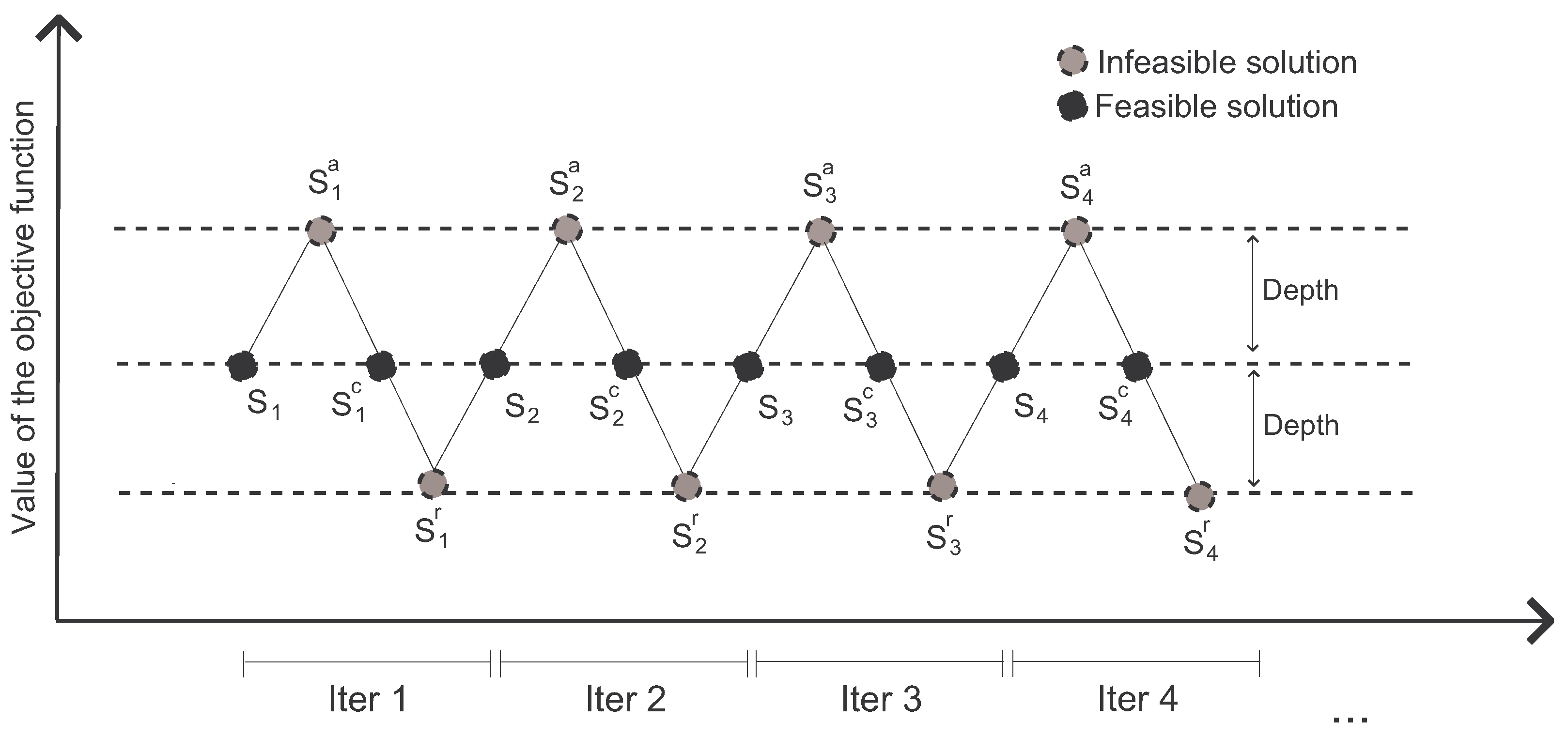
The Strategic Oscillation (SO) methodology was introduced by Glover [44]. The main idea of SO is to explore new regions of the solutions space by including infeasible solutions in the search. This behavior will eventually lead to new and high-quality solutions that are not possible to reach by just exploring the set of feasible solutions in a given neighborhood. Figure 2 illustrates the process of the SO algorithm. In the k-BCL problem, a feasible solution is represented as a set S of k selected facilities. Recall that the demand points have been assigned to its closest facility. Therefore, a solution is not feasible if the number of selected facilities is smaller or larger than k.

The method starts from an initial feasible solution $S_1$. Then, a new infeasible solution $S_1^a$ is generated by adding a certain number of new facilities to it. After that, the feasibility is corrected by oscillating again to a new feasible solution $S_1^c$, which is obtained by removing the number of facilities that excess from $S_1^a$. Next, the method moves to a new infeasible solution $S_1^r$ by removing facilities from $S_1^c$ and then finding a new feasible solution $S_2$ by including the required facilities to $S_1^r$ until it becomes feasible. Then, a new iteration begins, taking $S_2$ as its starting solution and repeating the same procedure as explained above.

Our SO proposal starts with a feasible solution S obtained using the GRASP algorithm (see Section 4.1 for details). The feasible solution with exactly k facilities is then destroyed by randomly adding $\beta ·k$ facilities, generating $S^a$; then, the feasibility is corrected by randomly removing $\beta ·k$ facilities, obtaining the solution $S^c$; then, the feasibility is destroyed again by randomly removing $\beta ·k$ facilities, generating $S^r$. The parameter $\beta$ is named the oscillation rate parameter, with $\beta \in [0,1]$, and it represents a percentage of the number of facilities that must be located in a feasible solution. Note that if $\beta =0$, solutions are feasible, otherwise, solutions are infeasible. In particular, the larger the value of $\beta$, the further from feasibility are the solutions generated. This parameter $\beta$ is responsible for controlling the balance between diversification and intensification in the SO algorithm. Furthermore, it is important to emphasize that each iteration of the SO each feasible solution obtained using the GRASP algorithm will generate two infeasible solutions with $k-\beta ·k$ and $k+\beta ·k$ facilities and one feasible solution with exactly k facilities.

Note that, as we are dealing with a multiobjective optimization problem, it is needed to check if every feasible solution obtained by the SO can be included in the set of efficient solutions and, if so, the set is updated.

4.3. Path Relinking

The Path Relinking (PR) algorithm is based on exploring trajectories connecting pairs of solutions (see [45,46,47], where PR is successfully applied). PR generates a trajectory that links an initiating solution ($S_i$) to a guiding solution ($S_g$). In other words, PR creates a path between two solutions by iteratively including in the initiating solution attributes from the guiding one. The rationale behind this idea is that a path from the initiating solution to a guiding solution will yield new solutions that share attributes from both solutions.

In this paper, we propose a novel application of PR: it is used as the repairing method inside the SO algorithm. In particular, PR is applied to generate a path between a pair of solutions that result from the infeasible solutions obtained in the SO. The initiating solution contains $k+\beta ·k$ facilities, while the guiding solution contains $k-\beta ·k$ facilities. Then, the path of solutions that connects them is produced by removing as many facilities in $S_i$ to make it feasible and then, performing exchange moves to include in $S_i$ elements that are not in $S_g$. Finally, the local search method described in Section 4.1.2 is applied to every feasible solution found in the path with the aim of finding new nondominated solutions.

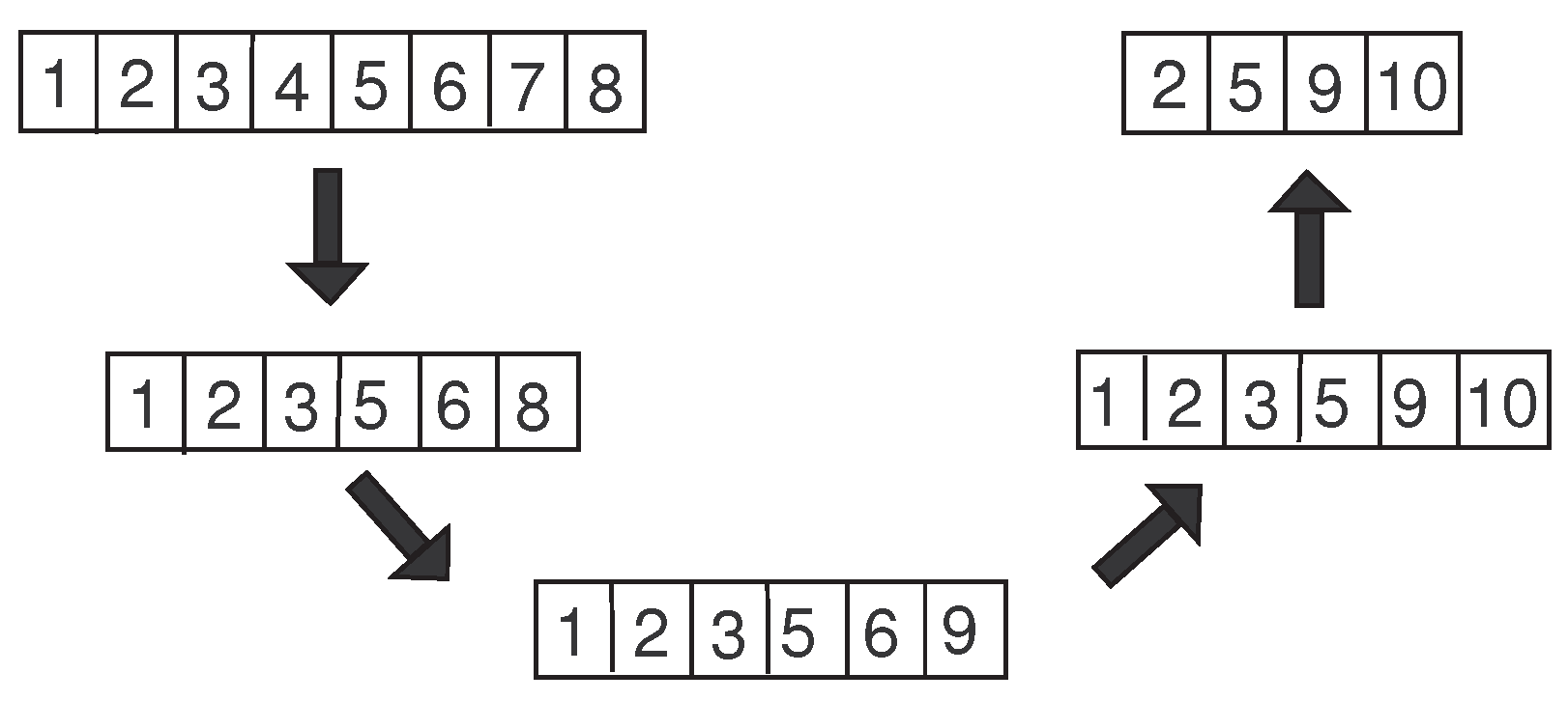
Figure 3 shows an example of how the PR works. Let $k=6$ be the number of facilities to be located in a feasible solution and $\beta =0.3$. We consider two infeasible solutions obtained with the SO methodology, specifically, let $S_i=\{1,2,3,4,5,6,7,8\}$ and $S_g=\{2,5,9,10\}$ be the initiating and guiding solutions with $k+\beta ·k=8$ and $k-\beta ·k=4$ facilities, respectively.

The candidate facilities to be removed from $S_i$ are those that are not in $S_g$, i.e., $R=\{1,3,4,6,7,8\}$, while the candidate facilities to be added to $S_i$ are those that are already in $S_g$ but not in $S_i$, i.e.,  $I=\{9,10\}$. The path between $S_i$ and $S_g$ is then created in two main phases: first, $\beta ·k=2$ facilities are removed to reach a feasible solution; then, a sequence of exchanges is performed until the incumbent solution of the path becomes $S_g$. The first phase results in $S_1=\{1,2,3,5,6,8\}$, obtained by removing facilities 4 and 7 from $S_i$. Then, $S_2$ is generated by removing facility 8, replacing it with facility 9. The last solution of the path, $S_3$, is reached by removing facility 6 from $S_2$ and inserting facility 10.

Notice that using Path Relinking as the repair method allows us to explore three new feasible solutions—namely, $S_1$, $S_2$, and $S_3$—from two infeasible solutions, increasing the portion of the search space explored. In this work, we propose the use of Path Relinking to combine every pair of two infeasible solutions, where the initiating solution contains $k+\beta ·k$ facilities and the guiding one contains $k-\beta ·k$ facilities, with the aim of finding new feasible ones in the path that connects them. As it is customary when we are implementing a multiobjective optimization problem, it is needed to check if the three new feasible solutions, $S_1$, $S_2$, and $S_3$, are efficient solutions; if so, they must be included in the set of efficient solutions, and therefore, all solutions of the set that are dominated must be removed.

5. Computational Results

In this section, computational results are presented and discussed to test the efficiency of the proposed algorithm, a hybrid SO with PR algorithm, henceforth, the SO+PR algorithm. All the algorithms are implemented in Java 11 and the experiments are conducted on a computer with a 2.8 GHz Intel Core i7 processor with 16 GB of RAM.

In the first set of numerical experiments, we use the same set of instances considered in the previous work [12]. Specifically, the author randomly selected $n=1000$ demand points in a rectangular workspace with size $1500\times 1000$ and $m=50$ potential facilities with the aim to locate $k=5,10,15,20,25$, and 30 facilities. Furthermore, we add two large-scale instances with $n=5000$, $m=500$, and $k=50,100$. These instances are used in the comparison with the three objective functions. Moreover, the author used for the comparison of the two objectives two nonuniform, large-scale problems named S1 and A3. The S1 instances have $n=5000$, $m=100$, and $k=10,30,50$, 80; the A3 instances have $n=7500$, $m=150$, and $k=15,45,75$, 120.

We compare the SO+PR algorithm with the previous one [12], named MOAkBCL, whenever possible. Then, in the final set of experiments, we compare our metaheuristic with several competitive evolutionary algorithms, specifically, NSGA-II [48], MOEA/D [49], and SPEA2 [50]. Note that the parameters of all algorithms have been set with irace [51], which automatically finds the best parameter settings of any algorithm. Furthermore, we have imposed an equivalent computational time to execute all the algorithms while avoiding any bias.

In multiobjective optimization problems, the performance of the methods involves computation of the efficient solutions. Then, to compare the quality among different algorithms, it is necessary to calculate basically three things: the cardinality of the obtained Pareto front, the proximity of the obtained solutions and the best/reference/optimal Pareto front, and the diversity of the obtained solutions. Note that, as the true Pareto front is unknown, a Reference Pareto front, R, is estimated merging all the nondominated solutions found by all the algorithms under comparison. Therefore, we use the following metrics to compare the multiobjective methods [52,53]:

• $\left|A\right|$—the number of efficient solutions.
• $C(A,R)$—the coverage calculates the proportion of efficient solutions of the Reference Pareto front, R, that weakly dominates the efficient solutions of the Pareto front obtained by the algorithm A.
• $\Delta$—the spread measures the distance between the efficient solutions obtained by the Pareto front of algorithm A, a perfect spread would be equal to zero.
• $HV$—the hypervolume evaluates the volume in the objective space, which is covered by the efficient solutions obtained by algorithm A.
• $ϵ$—the $ϵ$-indicator measures the smallest distance needed to transform every efficient solution obtained by algorithm A in the closest efficient solution of Reference Pareto front R.
• $GD$—the generational distance measures how far the efficient solutions of the Pareto front obtained by algorithm A are from those efficient solutions in the Reference Pareto front R.

It is worth mentioning that, in all the experiments, the best value for each metric is highlighted in bold font.

The first experiments consider the problem k-BLC${}_{123}$ and the compare SO+PR algorithm with Davoodi’s algorithm MOAkBCL, and with the most competitive evolutionary algorithms (SO+PR, MOEA/D, NSGA-II, and SPEA2). Here, we have considered three objective functions because, as Davoodi [12] holds, two different objective functions have been defined to measure the balance goal and even if they are not in conflict, they may result in different solutions. Therefore,

Table 3. Average results for the k-BLC${}_{123}$ on the WorkSpace and Large-scale instances. BCL—Balanced Center Location; SO—Strategic Oscillation; PR—Path Relinking.

	$\left|\mathit{A}\right|$	$\mathit{C}(\mathit{A},\mathit{R})$	$\Delta$	$\mathit{HV}$	$\mathit{ϵ}$	$\mathit{GD}$
MOAkBCL	6.00	0.78	0.98	0.26	1.31	133.43
SO+PR	10.88	0.17	0.96	0.40	0.06	105.56
MOEA/D	5.38	0.76	0.97	0.28	0.48	151.42
NSGA-II	7.50	0.57	0.96	0.35	0.56	126.34
SPEA2	7.13	0.58	0.98	0.36	0.61	131.54

shows the multiobjective metrics previously defined to compare the quality of the algorithms when solving the k-BLC${}_{123}$ problem on the WorkSpace and Large-scale instances. Results of this table illustrate that our algorithm outperforms the other algorithms since the SO+PR gets considerably better results in all the multiobjective metrics. The only metric that is similar is the spread, showing that the dispersion of the efficient solutions obtained by all the algorithms is quite similar.

Next, the results obtained when solving the k-BLC${}_{12}$ problem are included, also considering the instances used in Davoodi [12]. Following the same reasoning, we have solved the same problem considering just one balancing function. To that end,

Table 4. Average results for the k-BCL${}_{12}$ on the S1 and A3 instances.

	$\left|\mathit{A}\right|$	$\mathit{C}(\mathit{A},\mathit{R})$	$\Delta$	$\mathit{HV}$	$\mathit{ϵ}$	$\mathit{GD}$
MOAkBCL	5.63	0.26	0.93	0.28	0.80	177.73
SO+PR	5.38	0.33	0.84	0.17	0.86	184.15
MOEA/D	3.25	0.60	0.90	0.13	1.08	231.45
NSGA-II	3.13	0.74	0.90	0.12	1.11	229.44
SPEA2	2.25	0.72	0.84	0.13	1.04	254.66

compares the quality of the algorithms when solving the k-BLC${}_{12}$ problem on the S1 and A3 instances. The multiobjective metrics show that, on average, the MOAkBCL algorithm slightly outperforms the results obtained by the SO+PR algorithm. In order to prove if the results obtained by the MOAkBCL and the SO+PR algorithms are significantly different, we applied the Wilcoxon test. The p-values obtained are 0.673, 0.799, 0.025, 0.612, 0.779, and 0.674 for tests conducted on the number of efficient points obtained by each algorithm, the coverage, the spread, the hypervolume, the $ϵ$-constraint, and the generational distance, respectively. As we can see, considering a p-value equal to 0.01, there is no significant difference in the results obtained by both algorithms, which statistically demonstrates that both algorithms have a similar performance.

Having shown the performance of the proposed SO+PR algorithm over the test bed of instances proposed in the best previous method found in the literature, and with the aim of increasing the number of instances to have a more robust comparison, we propose the use of a new benchmark. This set of instances consists of 40 instances of the well-known OR-library (http://people.brunel.ac.uk/~mastjjb/jeb/info.html accessed on 1 December 2020) [54], named pmed instances, in which the number of demand points and candidate facilities are in the range of 100 to 900, while the number of selected facilities is in the range of 5 to 200. Since the source code of the previous algorithm is not available, we have included the evolutionary algorithms MOEA/D, SPEA2, and NSGA-II, which have already shown their potential for solving k-BCL. These instances have been shown considering k-BCL${}_{123}$ and k-BCL${}_{12}$, as in the previous experiments.

Results in

Table 5. Average results for k-BLC${}_{123}$ on the pmed instances.

	$\left|\mathit{A}\right|$	$\mathit{C}(\mathit{A},\mathit{R})$	$\Delta$	$\mathit{HV}$	$\mathit{ϵ}$	$\mathit{GD}$
SO+PR	6.87	0.26	0.93	0.44	0.13	32.60
MOEA/D	3.82	0.82	0.98	0.21	0.69	43.71
NSGA-II	4.31	0.72	0.98	0.25	0.65	42.27
SPEA2	4.62	0.74	0.97	0.24	0.55	40.54

and 

Table 6. Average results for k-BLC${}_{12}$ on the pmed instances.

	$\left|\mathit{A}\right|$	$\mathit{C}(\mathit{A},\mathit{R})$	$\Delta$	$\mathit{HV}$	$\mathit{ϵ}$	$\mathit{GD}$
SO+PR	4.73	0.27	0.93	0.45	0.22	34.56
MOEA/D	3.20	0.80	0.95	0.32	1.03	43.61
NSGA-II	3.08	0.78	0.96	0.31	0.76	43.83
SPEA2	3.30	0.68	0.97	0.39	0.76	41.97

show that SO+PR is the best algorithm for both multiobjective problems, k-BCL${}_{123}$ and k-BCL${}_{12}$. Our algorithm exhibits on average the maximum number of efficient points. Moreover, it obtains the lowest values in the coverage metric, the $ϵ$-indicator, the spread, and the generational distance, which compares favorably with the values of the evolutionary algorithms. Finally, if we focus on the hypervolume, SO+PR emerges as the best algorithm again, with a hypervolume of $0.44$ for the k-BCL${}_{123}$ and $0.45$ for the k-BCL${}_{12}$. In conclusion, all the metrics validate the conjecture that SO+PR outperforms the evolutionary algorithms for the multiobjective k-BCL problem.

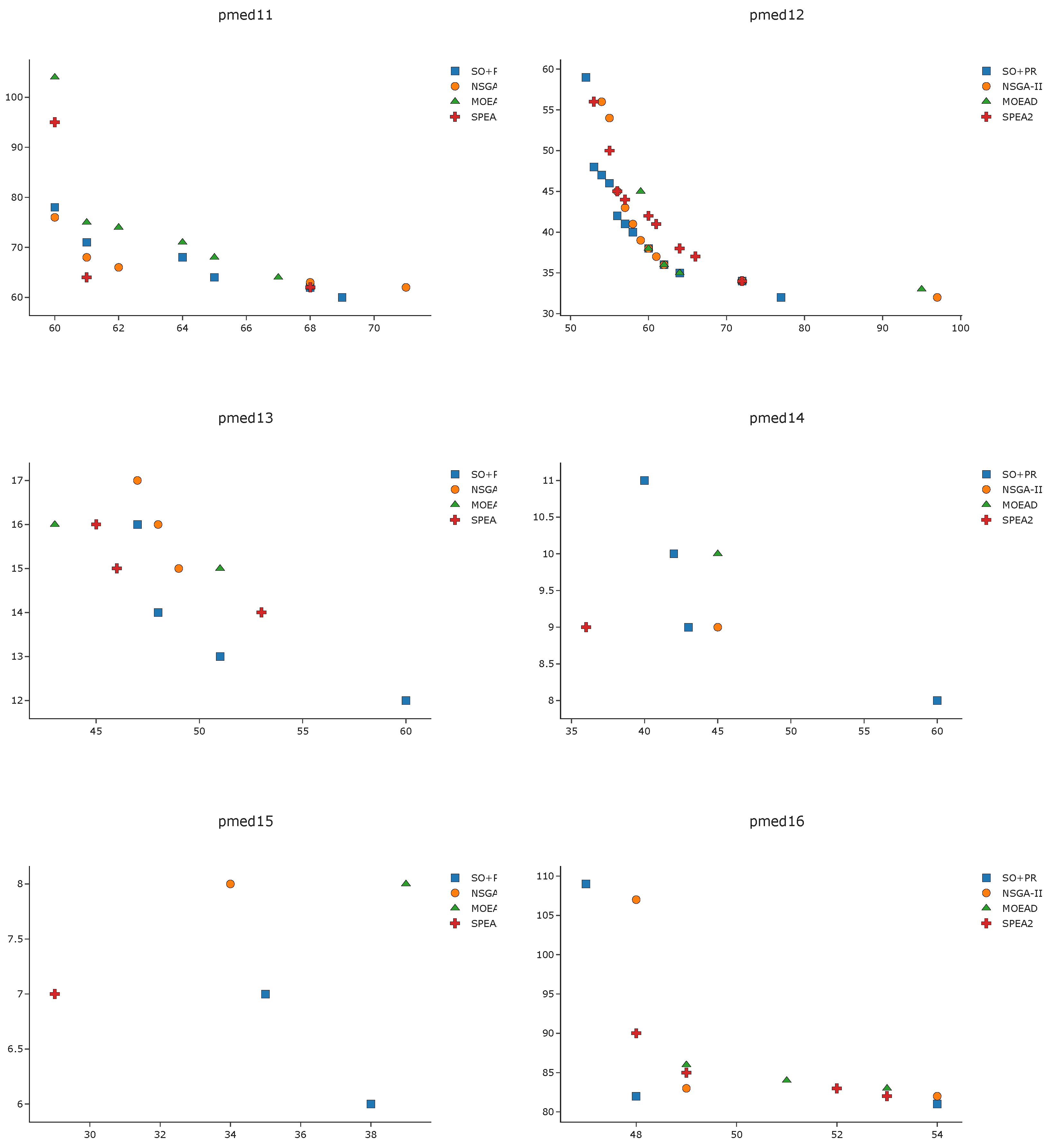
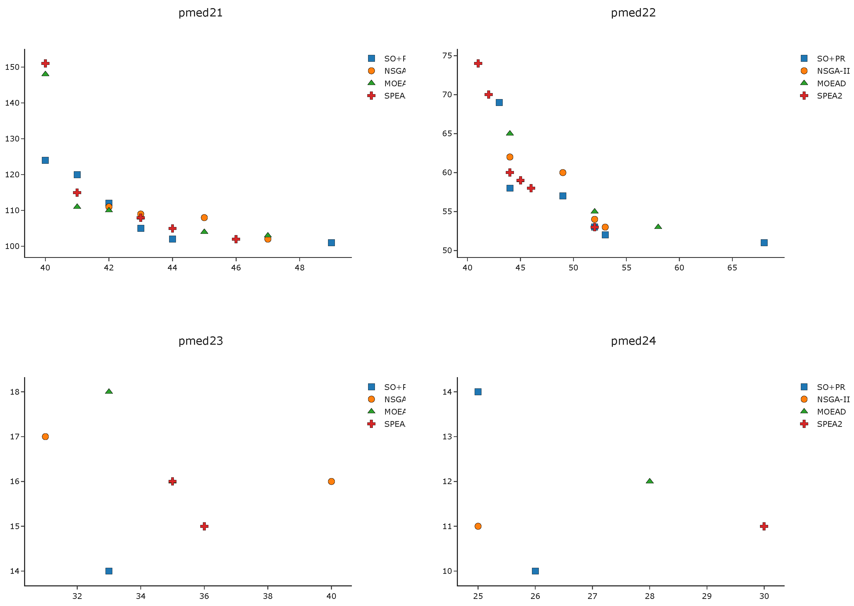
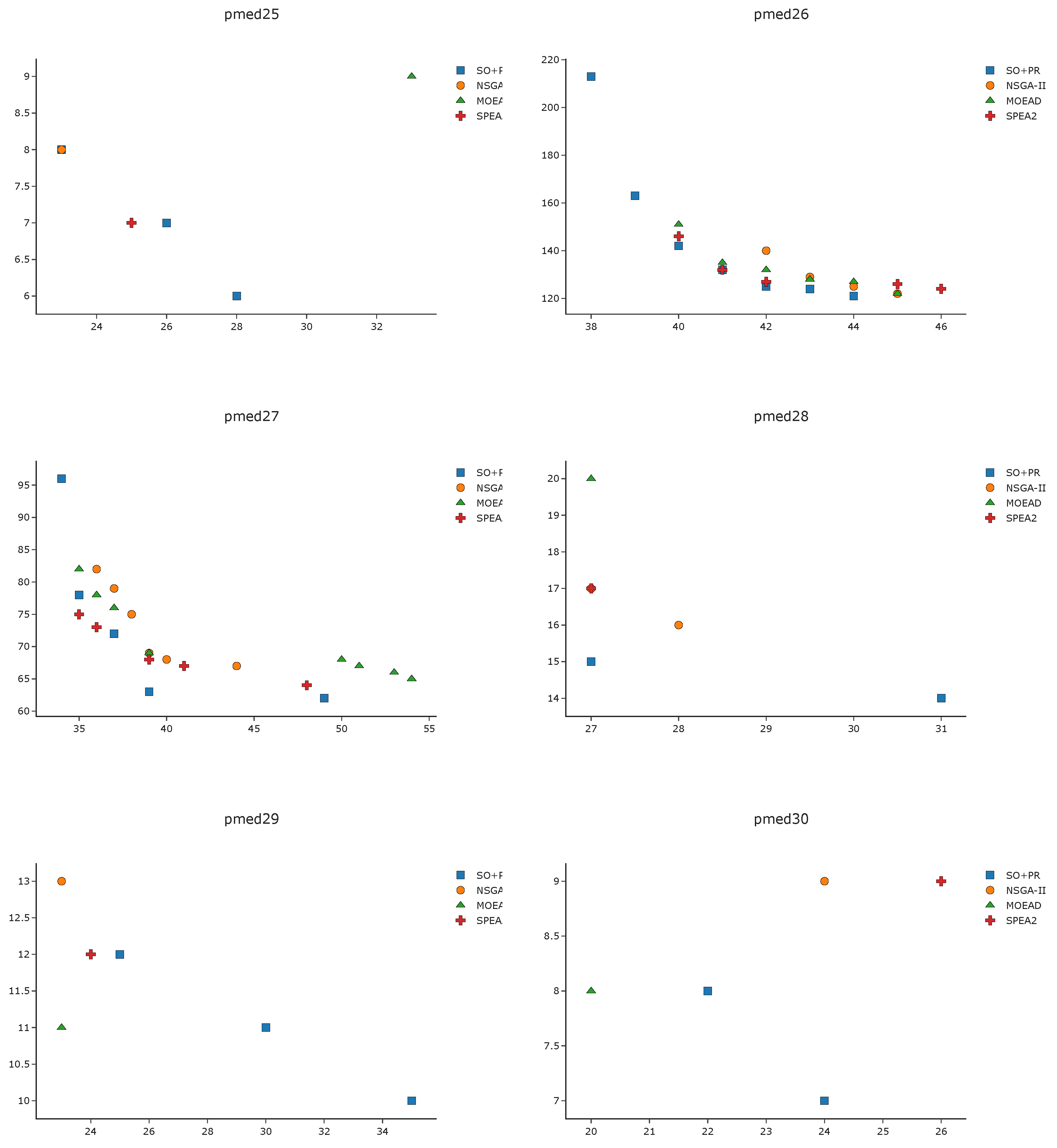
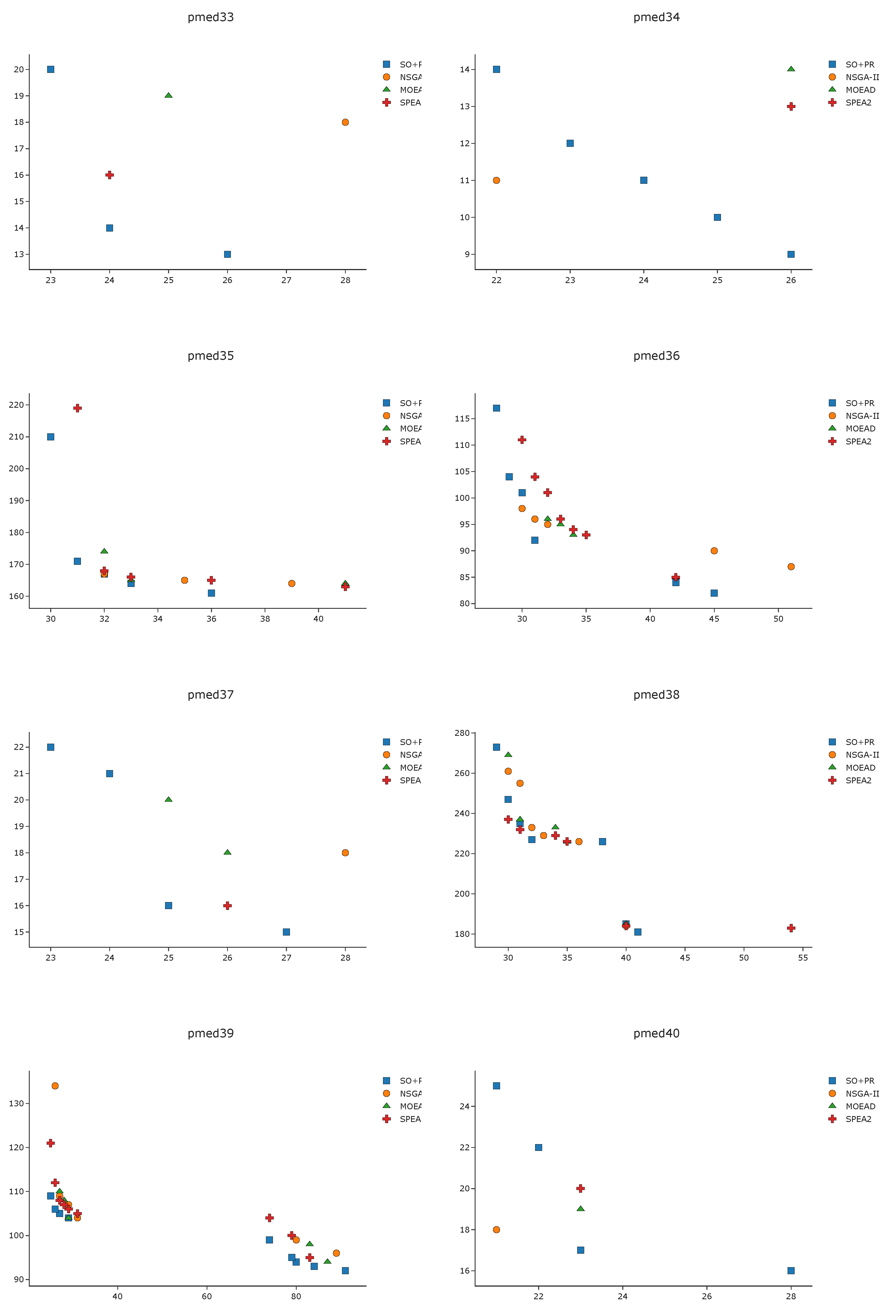
To complement the analysis of the results in the pmed instances, we depict in Figure A1, Figure A2, Figure A3 and Figure A4 the efficient frontier obtained with SO+PR, MOEAD, NSGA-II, and SPEA2 for k-BCL${}_{12}$. These figures illustrate the best approximation of the efficient frontier obtained by SO+PR with respect to the evolutionary algorithms.

6. Conclusions

In this paper, we have solved a novel multiobjective facility location problem, the k-Balanced Center Location (k-BCL) problem, that aims to locate a set of facilities optimizing two objectives at a time, the maximum distance between demand points and its closest facility and the balance of the workload of the facilities. We consider that the k-BCL is an important facility location variant that appears in many real-world problems, since the proximity of the located facilities to the demand points is as important as the workload of the located facility.

To solve the considered problem, we have proposed a new hybrid algorithm that combines Strategic Oscillation with Path Relinking. The proposal outperforms not only the state-of-the-Art algorithm but also the most competitive evolutionary algorithms—NSGA-II, MOEA/D, and SPEA2—proving the superiority of our algorithm. It is worth mentioning that using the Path Relinking algorithm for repairing the infeasible solutions generated by Strategic Oscillation, which have not been considered in the literature so far, leads to obtaining a set of high-quality efficient solutions.

As future research, it would be interesting to address new variants of this problem, studding different ways to measure the balancing function. To that end, we would follow the ideas of Barbati and Piccolo [22] but include the number of demand points instead of the distances. Additionally, we would like to explore the possibilities of hybridizing Strategic Oscillation with novel Path Relinking strategies, such as Exterior Path Relinking, to analyze the potential of these new hybridizations.