Abstract
This paper focuses on the last stage of the aluminium production process in the context of Industry 4.0: schedule optimization in the casting process. Casting is one of the oldest manufacturing processes in which a liquid material is usually poured into a mold that contains a hollow cavity of the desired shape and then allowed to solidify. This is a complex scheduling problem in which several constraints, such as different maintenance processes, maximum stocks, machine breakdowns, work shifts, or the maximum number of mold changes per day, come into play. Four objective functions have to be taken into account simultaneously. We have to minimize both the unmet demand at the end of the schedule, and the delays in the injection process with regard to daily demands. Production costs, including the cost of electricity consumption in the injection process and gas consumption associated with melting furnaces, should be minimized. Finally, the total number of mold changes throughout the schedule must also be reduced to a minimum. The simulated annealing (SA) metaheuristic has been adapted to solve this complex optimization process and parameterized for application to a wide variety of aluminium making processes. SA efficiently solves the problem and provides an optimal solution in about three minutes.
1. Introduction
Today’s organizations are embracing Industry 4.0, the fourth industrial revolution, which combines advanced manufacturing and operations techniques with emerging smart technologies, ranging from robotics, artificial intelligence, cognitive technologies, nanotechnology to the Internet of Things. Industry 4.0 leads to a continuous cycle, where a real-time flow of information and actions from heterogeneous sources and sites are networked according to a cyclical physical-to-digital-to-physical (PDP) process. The iterative PDP steps are as follows:
- Digitally record the information captured from the physical world.
- Share information and apply advanced analytics, scenario analysis and artificial intelligence to discover which information is applicable.
- Apply algorithms to translate digital world decision making into real data.
This PDP process should stimulate actions and changes in the physical world.
In this paper, the PDP cycle has been adapted to tackle the last stage of the aluminium production process, schedule optimization of the casting process.
The steel-making and aluminium production process is composed of different stages [1]. First, steel or alumina is smelted in an electric arc furnace, then the liquid metal is poured into a ladle with some additives to obtain the desired chemical composition of the product. The metal then undergoes the vacuum degassing process, which reduces hydrogen and nitrogen gases dissolved in the molten aluminium to improve the quality of the final products. Finally, the steel or aluminium is cast.
Casting is one of the oldest manufacturing process, where a liquid material is poured into a mold that contains a hollow cavity of the desired shape and then allowed to solidify. It is most often used to make complex forms that would otherwise be difficult or uneconomical to produce. Casting components can vary in size, from the tiniest component of the size of an ant to huge components weighing tons. Various types of casting processes are available based on the type of mold and how the molten metal is filled, like sand casting, die casting, continuous casting, squeeze casting, investment casting, etc.
The success of all these casting processes depends on the close and proper control of all the input parameters and the metal solidification process. As the casting process involves advanced technologies, just a small variation in any of the input parameters can affect the process output and produce defective castings. Hence a lot of effort is being made to develop mathematical models to achieve exact parameter settings instead of using trial and error. This can be achieved using advanced optimization techniques as tools to output the optimum parameter setting for the casting processes under consideration. A comprehensive literature review about casting process optimization issues is reported in Reference [2], highlighting the urgent need for research into process parameters and process optimization.
For instance, three important casting processes, namely squeeze casting, continuous casting and die casting process, are considered in Reference [3], and the teaching-learning-based optimization (TLBO) algorithm is used to optimize mathematical models of these processes in Reference [4].
More recently, the performance parameters of sand casting were optimized on the basis of grey relational analysis and the missing data predicted using a back propagation (BP) neural network [5], whereas [6,7] deal with the optimization of die and squeeze casting processes, respectively, based on the Taguchi approach, and [8] focuses on thermal optimization of the continuous casting process using a distributed parameter identification approach.
Optimized scheduling is of crucial importance to ensure productivity and competitiveness in the steel-making and aluminium production processes. There is an extensive literature on production planning and scheduling in the steel industry. Reference [9] provides a comprehensive and comparative analysis of early works. Since then, different versions of the steel-making and casting scheduling (SMCP) problem have been considered by different authors. A review is available in Reference [1], grouped according to mathematical programming methods, constraint programming methods and metaheuristic and hybrid methods. Within the first group of mathematical programming methods, researchers proposed solutions ranging from the first SMCP [10], a multi-objective integer linear programming (MILP) model [11], a Lagrangian relaxation for machine capacity and job precedence constraints based on an approximate subgradient algorithm [12]. Constraint programming methods were reported in References [13,14,15], whereas metaheuristics and hybrid methods ranged from tabu search [16], evolutionary programming [17], artificial bee colony algorithms [18], simulated annealing [19,20], genetic algorithms [21] or particle swarm optimization (PSO) [22].
In Reference [23], a steel-making-continuous casting scheduling model is considered, where due dates are just-in-time-based interval type-2 fuzzy random variables, and the corresponding type-2 fuzzy random optimization problem is transformed into a crisp and nonlinear optimization problem using the symmetric approach.
More recently, a simulation annealing approach was developed to tackle a general model combining common features and constraints on the operations of a real plant [1]. Specifically, it is a complex variant of the hybrid flowshop problem [24] with sequence-dependent setup times and heterogeneous processing times. The aim is to select the jobs from a large pool of orders, assign them to machines and plan the sequencing and timing, maximizing the number of jobs whose processing starts within the corresponding time horizon.
A similar version of the problem considered in Reference [1] was previously addressed in Reference [11], where a MILP formulation was used with the makespan as the objective function.
The current state and recent developments of plant coordination and control, raw materials and energy optimization and quality management in the steel industry is reviewed in Reference [25], discussing the future methods and developments.
In this paper, we focus on the last stage of the aluminium production process, namely schedule optimization in the casting process, rather than the whole process considered in References [1,11]. Specifically, different injection machines pour aluminium into molds including one or more parts. As there is a person who is in charge of reloading the injection molding machines, we can assume that the aluminum for injection is always on hand, and aluminium availability does not, therefore, constitute a constraint.
The optimization process will account for four objective functions simultaneously. The first two objectives refer to orders. On the one hand, we have to take into account delays with respect to daily part orders and, on the other, orders that are not met on schedule. Initially, unmet parts orders and parts order delays will not be prioritized, the aim being to minimize the total sum of unmet orders and delays. Besides, production costs also have to be reduced to a minimum, and we consider the cost of electricity consumption in the injection process and gas consumption associated with the melting furnaces. Finally, the number of mold changes must be minimized. The four objectives are normalized and incorporated into a weighted additive fitness function, where the weight represents the relative importance of the objectives.
We have to decide which molds have to be loaded and removed from the injection machines during the two-week schedule, taking into account different constraints associated with the injection process (maintenance processes, planned machine downtime, maximum stocks of parts, work shifts, maximum mold changes per day, non-working days, etc.). The goal is to reach a feasible solution that minimizes the above fitness function. To do this, we use the simulated annealing metaheuristic [26,27].
The paper is structured as follows. Section 2 details the aluminium parts casting process under consideration. The adaptation of simulated annealing to the optimization problem is described in Section 3. Section 4 illustrates the application of SA to a real instance together with the parameter settings in the SA, and analyses results. Finally, some conclusions are outlined in Section 5.
2. Problem Description
The company has several injection molding machines powered by electric holding furnaces, which in turn are fed by propane gas melting furnaces. There are a total of n molds, in which we can inject different parts. Specifically, there are molds that have a single part, most have two parts (50% of each type) and there is a mold for casting three different parts.
An allocation (binary) matrix indicates, for each injection molding machine, which molds can or cannot be used to inject parts. The injection time for each mold depends on the specific mold, but not on the processing machine. Injection times are of the order of seconds, but our problem is structured according to minimum one-hour production processes in which several consecutive mold injections are made. The number of parts that are injected per hour in each mold is known.
As there are several copies of some molds and molds that produce several parts, the same part may be injected on several machines simultaneously using different molds. Mold change times range from 1 to 2 h, but they are all rounded to 2 h and do not depend on the machine or the particular mold. We assume that the first hour of the change time is to remove the mold and the second to mount the new mold. There is a maximum number of mold changes () that can be performed (on all machines) per day. Mold changes cannot be performed simultaneously on multiple injection molding machines, since there is only one workgroup that performs the changes one by one. No mold change time has to be considered for consecutive injections of the same mold on the same machine. A mold change that takes place over a two-day period, that is, between 23:00 on Day 1 and 1:00 on Day 2, will be accounted for on Day 2. Mold changes are always made within one work shift: they cannot start during one shift and end during another. Therefore, a mold change cannot be started during the last hour of each shift. The shifts are as follows: 07:00–15:00, 15:00–23:00, and 23:00–07:00. Therefore, changes from 6:00 to 8:00, from 14:00 to 16:00, or from 22:00 to 20:00 are not allowed.
We assume that the molds that were being used on the different machines at the end of the two-week schedule are already in place and must be taken into account (as model input) for the next schedule. This is the only information that is carried over from one schedule to another, although orders not met in one two-week schedule are incorporated into the early stages of the next schedule to minimize production delays.
The injection molding machines work 24 h a day but require maintenance. Melting furnace maintenance takes three days, whereas holding furnace maintenance takes one day. During melting furnace maintenance, the associated machines operate at of their capacity. On the other hand, during the one-day maintenance of the holding furnaces, aluminum cannot be produced (injected) in the associated machines. In the first case, we use a maintenance (binary) matrix, including the maintenance days in the two-week schedule. In the second case, we take into account whether the maintenance time slot is fixed or varies and then process the data input accordingly. Maintenance cannot be performed on non-working days.
When the maintenance starts, the mold is not removed from the respective injection molding machine if production is to be continued. We have assumed that the mold is left in place on non-working days or during planned downtime.
We have the option of an extra 24-h shift on each day of the weekend or on public holidays (divided into two 12-h shifts: from 7:00 to 19:00 and from 19:00 to 7:00 on the following day). A binary vector is used to indicate which of the days of the two-week schedule are working days and which are not (public holidays or weekends). This information is incorporated into the maintenance matrix, and each public holiday is equivalent to a one-day maintenance operation (i.e., the injection molding machine is out of service) on all the machines. All the times considered in the model are integer values. Therefore, the time is discretized in one-hour intervals.
On the other hand, some injection molding machines might be in operation and others might not on weekends. This will also be a model input. The schedule can start on any day of the week, not necessarily on a Monday, but will cover the following two-week period as of that day. Finally, the schedule can start at any time on the first day, which is another model input.
There is a maximum stock of stored parts at the end of the week. This will be different for the different manufactured parts. The first week’s initial stock is not disregarded since it is accounted for by the orders for the two-week schedule. Therefore, the stock at the end of the first week is calculated based on the surplus production of the part with respect to the total weekly demand for that part, after subtracting defective manufactured parts (the proportion of defective parts is known for each type of part), whereas, for the second week, it is calculated as the initial stock of the respective part (that is, the stock of that part at the end of the first week), plus the number of parts that have been injected during the week, minus the defective injected parts. The schedule covers a two-week period, although the parts orders are calculated daily and maximum stocks are counted weekly.
Machines may break down. To deal with this problem, a percentage of the available weekly production hours should be set aside as planned downtime to account for such breakdowns. Once the failure has been fixed, production takes place during planned downtime. Planned downtime is set aside at the end of the schedule. If no malfunctions occur, planned downtimes could be used to inject additional parts. Planned downtime is not necessarily the same for all machines, although it is initially set at across the board.
The quantity of aluminium available (kg) for the injection molding machines does not constitute a constraint, since there is a person who is in charge of reloading the machines and we can assume that injectable aluminum is always available.
We take into account four main objective functions simultaneously. Two of the objective functions refer to the failure to meet part orders, whereas the other two are concerned with production costs and the number of scheduled mold changes, respectively. A weight vector representing their relative importance will be a model input.
Regarding order satisfaction, we must take into account both delays that occur with respect to daily orders and orders that are not filled by the end of the schedule. Initially, unmet parts orders and parts order delays will not be prioritized, the aim being to minimize the total sum of unmet orders and delays. Note that a weighted additive objective function could quite easily be added in the future for the purpose of prioritization.
Regarding production costs, we consider the cost of electricity consumption in the injection process where consumption only occurs when the machines are injecting molds, but not during mold changes, maintenance, or simply stoppages (if any). The gas consumption associated with melting furnaces must be added to the above.
3. Problem-Solving Methodology
Simulated annealing (SA) [26,27] is a trajectory-based metaheuristic method inspired by annealing in metallurgy, which has been adapted to solve many combinatorial optimization problems [28,29,30], and with both general and problem-specific improvements and variants over the years [31].
The basic idea of SA is as follows, see Algorithm 1. An initial feasible solution, , is randomly generated. Then, in each iteration i, a new solution () is randomly generated from the neighborhood, , of the solution considered in that iteration, . If the new solution is better than the current one, then the algorithm moves to that solution. Otherwise, there is a given probability of it moving to a worse solution. The acceptance of worse solutions makes for a broader search for the optimal solution and avoids trapping in local optima in early iterations.
The search is initially very diversified, since practically all moves are permitted. Then, the probability of accepting a worse move decreases as the temperature drops, and only better moves are accepted when it is zero, working like a hill-climbing algorithm in the last iterations.
Some elements in the above algorithm require clarification. Generally, the initial temperature () is set such that the acceptance ratio of worse moves is equal to a specified value, [32].
The cooling schedule defines the way in which the temperature decreases across iterations. A common cooling schedule is for the temperature to be kept constant for a number of iterations (L) and then be decreased according to a geometric schedule: , the typical value for being 0.95 [33].
The most commonly used stopping criterion is to stop when the improvement in the fitness function is less than a given percentage for a fixed number of iterations.
In the following sections, other elements of the SA algorithm are explained in detail, including how solutions are modeled (), how an initial feasible solution is built and the neighborhood definition considered ().
3.1. Solution Modeling
Solutions are represented by a matrix. The matrix columns represent time slots, and the rows, injection molding machines (). Time slots are equivalent to one hour, as demanded by the experts, since this is the minimum mold injection time, and we can assume that the duration of injection processes is measured in multiples of hours. Consequently, as we have a two-week schedule, the solution matrix is composed of 24 (h) × 14 (days) = 336 columns.
| Algorithm 1 Basic SA. |
|
Each matrix element represents the state of the injection molding machine i in time slot j. It is symbolized by a numerical value. The value 0 indicates that the respective injection molding machine is stopped, values 1 to n state that mold is being injected in the respective time slot on the respective injection molding machine, value refers to a non-working day slot time, value and denote three-day and one-day maintenance processes, respectively, value represents a mold change and value specifies planned downtime. Colors are also used to improve solution interpretability, see Figure 1.
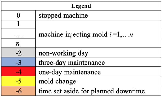
Figure 1.
Solution modeling.
Figure 2 illustrates the modeled solution. The solution includes six injection molding machines (6 rows) and only shows the first two days out of the two-week schedule accounted for by the modeled solution. Molds 1, 4, 6, 9, 15 and 3 are injected in the six injection molding machines under consideration at the beginning of the solution, respectively. Mold 1 is injected on injection machine 1 on the first and second day until time slot 7 on the third day. Then, mold 1 is replaced by mold 2. Besides, a three-day maintenance process starts on injection machine 2 on the second day. Mold 15, initially injected on injection machine 5, is replaced by mold 16 at time slots 6 to 7 on day 1. Mold 16 is then replaced by mold 6 at time slots 4 to 5 on day 2. Then, a three-day maintenance process starts on day 3.
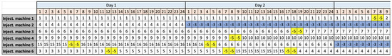
Figure 2.
Illustration of a part of a solution.
3.2. Building an Initial Solution
Although we have daily parts orders, we build the initial solution assuming that demand is accumulated at the end of each respective week of the two-week schedule. Besides, production costs are not considered in this process.
Initalization. We first set all the elements in the solution matrix to 0, that is, initially all the machines are stopped. Then, we enter the value −2 in columns representing public holidays or weekends where production is stopped. To do this, we take into account a non-working day vector (input). For instance, the non-working day vector (0, 0, 1, 0, 0, 0, 0, 0, 0, 0, 0, 0, 1, 1) indicates that there is a public holiday on Wednesday of the first week and the second weekend.
In the case of weekends, where some injection molding machines operate and others do not, we also enter the value −2 for the machines that are not operational on weekends.
We assign the value −4 for the elements associated with machines under one-day maintenance, whereas machines undergoing three-day maintenance are marked −3 because they are operating at only c% of their capacity, taking into account the maintenance matrix (input) in both cases. Finally, we enter −6 in the column cells at the end of the solution matrix set aside for planned downtime to cover machine breakdowns.
The initial solution is built in two phases, each considering one of the two weeks of the schedule. For the first week, we proceed as follows: we complete the solution matrix row by row, starting with the first machine and performing injections with molds for the most demanded parts, if possible, and mold changes when necessary, also taking into account molds availability (i.e., they are not being used on another machine), maintenance processes and non-working days.
- for to (for each injection machine)
- −
- −
- −
- WHILE ( and ) (until the end of the week (7 days h or the stopping criterion is met)
- *
- If ( or then (the machine is under one-day maintenance or not in service because it is a non-working day. We move to the next day).
- *
- Else, for each mold j that machine m can inject (consult the injection matrix) and by order of the accumulated demand for the parts during this week (using the mold that can cast more of the most demanded parts first…), do
- ·
- If the injection conditions (specified afterwards) are met, then- (perform a mold change). If the mold that was being used during the previous hour is not the same as the one that is going to be loaded, then we remove the previous () = −5) and load the new mold (, ), i.e., a two-hour mold change is performed. Else (no mold is loaded on the machine), we just load the new mold ().- (perform the injection). Inject mold j on machine m until the maximum stock of the parts being injected is exceeded (, until the end of injection). The injection could end before if mold j is used on another machine in the future (in an already processed machine, ). Note that we must check if machine m is undergoing a three-day maintenance process, i.e., working at of its capacity. Besides, if there is a one-day maintenance process or a non-working day before finishing the injection, then injection continues afterwards until it is completed.- Reduce the demand for the parts in the mold by the number of injected parts and update the respective stocks (if necessary).- Increase h to the time just after the end of the injection.
- ·
- Else (at least one injection condition is not met), try with the following mold that machine m can inject in the order of demand for parts. Note that there may be several molds with the most demanded part, and they should all be used until the maximum stock is reached.If no mold can be injected, then .
- −
- end_WHILE
- −
- end_FOR
The algorithm is the same for the second week, but we first have to update the parts orders for this week with the stocks of the parts at the end of the first week. Besides, the stopping criterion will be met when either no mold can be injected or the algorithm reaches a planned downtime.
The injection conditions mentioned in the above algorithm are as follows:
- Check that the mold under consideration is not being used (or is being changed and mold injection begins on another machine) on another machine (previous rows in the solution matrix) for the next three hours (minimum time necessary to perform a mold change and at least one injection).
- Check that the maximum storage stock of the parts included in the mold produced during week 1 will not be exceeded after the planned injection.
- Check that the maximum value for mold changes per day is not exceeded (this is not a problem if no mold change is required but must be checked if there are mold changes) or that they are not being carried out during shift change hours (4:00 to 5:00, 12:00 to 13:00 or from 20:00 to 21:00).
Note that initial solutions generated may differ if the machines to be injected (rows) according to the algorithm are randomly selected.
3.3. Neighborhood Definitions
The simulated annealing algorithm takes into account three neighborhood definitions: completely remove an injection, partially remove an injection, and add an injection.
In the first neighborhood definition, completely remove an injection, a randomly selected injection is completely removed from the respective machine. This process also implies removing the mold change hour before and after the respective injection process. The process is a follows:
- Randomly select a machine m.
- Randomly select an injection process (mold i) on machine m.
- Set to 0 all the hours corresponding to the injection process under consideration.
- Set to 0 the mold change hour just before and after the removed injection (they are associated with the process of loading and removing the mold at the beginning and end of the injection, respectively).
- Update the weekly stock of the parts included in the removed mold i (possibly more than one part). For each part, either subtract the quantity of the part that is not to be injected from the stock or set to 0 if the number of parts that are not injected is greater than the available stock. Be sure to update the stocks of both weeks if the removed injection covers the entire two-week schedule.
- Update the fitness functions for the new solution: decrease the demand (at the end of the two weeks) satisfied for each part in mold i, decrease the cost of the new solution since no electricity and gas will be paid for the injection of the removed mold i on machine m, and update delays in production regarding the daily orders (this complex task involves recomputing delays for the entire schedule).
Figure 3 shows an example of the application of this neighborhood definition, in which injection of mold 5 is completely removed.
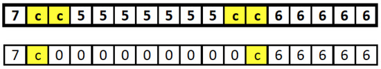
Figure 3.
Examples of neighborhood definition 1.
In the second neighborhood definition, partially remove an injection, a part is removed at the beginning of a randomly selected injection process. The length of the injection removed is also selected at random. In this case, the mold change hour is moved from the beginning of the injection process to the new mold loading time at the end of the removed injection time. Figure 4 shows an example of the application of this neighborhood definition, in which the injection of mold 5 is partially removed.
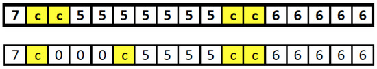
Figure 4.
Examples of neighborhood definition 2.
In the third neighborhood definition, add an injection, the injection of a randomly selected available mold is added in a randomly selected gap (during which the machine is stopped) of a randomly selected machine m. The new injection covers the entire gap, and a mold change hour must be added at the beginning and end of the injection process to load and remove the respective mold. Note that it is important to check if the selected mold i was being injected just before or after the new injection, in which case no mold change will be necessary.
Now, the mold change hour at the beginning of the injection process is removed and added at the end of the removed hours, which is when the mold is loaded. Figure 5 shows examples of the application of this neighborhood definition.
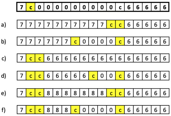
Figure 5.
Examples of neighborhood definition 3: (a) corresponds to an injection with the same mold that was used before the gap and covers the entire gap, where the mold used afterwards is different, (b) is the same as (a) but the gap is not completely covered, where the mold has to be removed leaving a smaller gap, (c) corresponds to an injection of a different mold than the one used before the gap, covering the entire gap, where the same mold is used afterwards (there is no change of mold at the end of the gap), (d) is the same as (c) but the gap is not completely covered, where the mold is removed leaving a smaller gap, (e) corresponds to an injection of a different mold from the one before and after the gap which covers the entire gap, and, finally, (f) is the same as (e) but the gap is not completely covered, where the mold has to be removed leaving a smaller gap.
3.4. Fitness Function
As already mentioned, the optimization process will take into account four objective functions simultaneously. The first two objectives refer to demands. Orders that are not met by the end of the schedule should be minimized, whereas delays with respect to the satisfaction of daily part demands must also be taken into account. Initially, neither unmet parts orders and delays will be prioritized. Therefore, the total sum of unfufilled orders and of delays will be minimized.
Regarding the production costs (), electricity pricing is made up of a power capacity and electricity consumption (fixed term and variable term). Power capacity is calculated on an annual basis averaged per month (we do not take into account this cost). We take into account electricity consumption, but not the surcharge for power peaks above 2450 kW. We also consider the gas consumption associated with melting furnaces.
Finally, the number of mold changes () in the planned period must be minimized.
The four objectives are incorporated into a weighted additive fitness function, where the corresponding weights represent their relative importance according to the experts’ preferences:
To do this, the objective functions must be normalized, since they are measured in different units with different value ranges:
where
and is the total parts demand during the two-week schedule, are the accumulated delays if parts are not injected, represents the solution in which all machine molds are injected with maximum amount of aluminium across the two-week schedule and accounts for a solution with the maximum permitted mold changes per day () on the all working days.
Note that the fitness for each visited SA solution is not computed from zero. Instead, we merely compute how the movement dependent on the respective neighborhood definition affects the fitness function of the previous solution (although the updated delays have to be recomputed for the entire solution). This improves the algorithm from a computational point of view.
3.5. Parameter Tuning
Different instances of the problem were used to set the SA parameters and improve its performance. Different stopping criteria and cooling schedules were tested together with the probability of using the three neighborhood definitions. Several graphs about the evolution of the fitness value, its optimal value, and the probabilities of worse movements were plotted to check that the search process evolved adequately.
As a result of the above analysis, the SA parameters were set to the following values: stopping condition (, ), cooling schedule (, ), and neighborhood probabilities (complete removal 0.1%, partial removal 0.4%, insertion 0.5%).
4. An Illustrative Example
In this illustrative example, we consider aluminum injection molding machines, powered by electric holding furnaces, which in turn are fed by four propane gas melting furnaces. There are 84 available injection molds, including molds for a single part, two parts or three different parts. Of the 173 different parts that can be injected, only 33 are ordered during the two-week schedule, where the total demand for parts is 224,864. Note that parts that are not in demand could be injected if they are in the same mold as an ordered part. Table 1 specifies the molds including the 33 ordered parts, together with the number of parts and quantity of aluminium (kg) injected per hour.

Table 1.
Mold information.
We assume that there are no stocks and no molds are loaded on the six injection machines at the beginning of the schedule. The first Sunday and the second weekend are non-working days, whereas only injection machines 1, 4, and 5 are available on the first Saturday. There is a three-day maintenance process on machine 1 from Wednesday to Friday during the first week ( operating capacity), and a one-day maintenance on machine 2 on Tuesday during the first week.
Up to four mold changes are permitted per day (). Mold changes must not be simultaneous or overlap with shift changes (6:00–8:00, 14:00–16:00, and 22:00–24:00). Planned downtime for machine breakdowns accounts for of the schedule.
Regarding the production costs (), electricity pricing is made up of a power capacity and electricity consumption (fixed term and variable term). Power capacity is calculated on an annual basis averaged per month (we do not take into account this cost). We take into account electricity consumption, but not the surcharge for power peaks above 2450 kW. We also consider the gas consumption associated with melting furnaces.
The consumption in kWh of the six injection molding machines is computed for machine 1 as follows:
where is the number of kilograms of aluminum injected per hour into the mold that is being used on machine i. Similar expressions are used for the other machines.
Figure 6 shows the price in euros per kWh consumed for each of the 24 h of the day (from Monday to Friday) over the different months of the year. The price per kWh consumed on Saturday, Sunday, or public holidays is euros irrespective of time of the day.
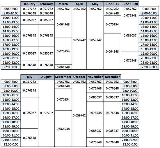
Figure 6.
Electricity billing term.
Regarding gas consumption in melting furnaces (4 furnaces), we have for melting furnace 1:
Note that injection machines 1, 2 and 3 are fed by melting furnace 1, whereas injection machines 4, 5 and 6 are fed by melting furnaces 2, 3 and 4, respectively. Similar expressions are used for the other melting furnaces. The cost of gas per kWh is 0.13 euros.
Weights representing the relative importance of the objective functions in the normalized fitness function were provided by the casting company’s expert (, , , respectively), i.e., the first two objectives concerning orders are much more important than operating costs and the total number of mold changes.
The schedule starts on Monday at 13:00 h. A first feasible solution is derived from the algorithm described in Section 3.2, whose fitness value is . The total unmet demand in the two-week schedule is 540 parts, amounting to 0.24% of total demand, the total delay (units × days) is 83.092, the operating costs are 21,552.37 euros and the total number of mold changes is 19.
Then, SA is executed to derive an optimal solution. Figure 7 shows the evolution of both the fitness function and the four original objective functions throughout the execution. We find that the search is very diversified at the beginning of the execution, since practically all moves are permitted. As the temperature drops, the probability of accepting a worse move decreases, and the search becomes more intensified, working like a hill-climbing algorithm at the end when only moves that improve the fitness function are allowed. A total of 301.499 iterations were performed before the algorithm stopped. We used an Intel(R) Xeon(R) E3-1240 PC with 3.50 GHz and 16 GB of RAM, running Windows 10, and the execution time was 3 min.
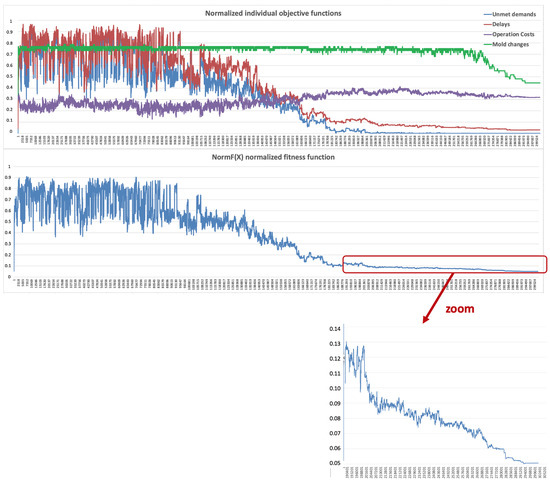
Figure 7.
Simulated annealing (SA) evolution.
The fitness value for the optimal solution is . The total demand (224,864 parts) is met according to schedule, the total delay (units × days) is 55,351 (there are delays for only 14 out the 33 ordered parts), the operating costs is 20,630.84 euros, and the number of mold changes is 25.
Figure 8 shows the first three days for the optimal solution. As already mentioned, the schedule starts on Monday at 13:00 h when no molds are loaded on any of the six machines.
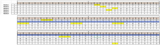
Figure 8.
Part of the optimal solution.
During the first hour (13:00), mold 79 is loaded on machine 1, which is injected until the time slot 4 on the second day, when it is replaced by mold 62, used until the end of day 2. Then, a three-day maintenance process starts on Wednesday, where the machine continues to inject mold 62, but only at of its capacity.
Besides mold 7 is loaded on injection machine 2 at 14:00 h. Note that mold changes cannot be performed simultaneously on more than one machine. Mold 7 is injected on machine 2 until 20:00 on which it is loaded but not injected from 20:00 to the end of the day. Then, machine 2 undergoes a one-day maintenance operation on Tuesday, and mold 7 is again injected from 0:00 to 7:00 on Wednesday, when it is replaced by mold 44, which is injected for the rest of the day.
Table 2 and Table 3 show further details about the optimal solution. The first two columns list part numbers and the respective maximum stocks. Note that Table 2 and Table 3 list more than 33 parts (rows), since they include all the parts injected over the two-week schedule and not only the ordered parts.
Table 2.
Optimal solution I.
Table 3.
Optimal solution II.
The following three columns show the aggregate orders over the first week (note that orders are received on a daily basis), the number of parts injected, and the stock (positive) or unmet demand (bold-red-negative) at the end of the respective week. The following three columns show the same information for the second week. Note that the demand for seven parts is not met at the end of the first week, leading to delays, but the demands for these parts is met at the end of the second week. Moreover, the demand for all parts over the entire two-week schedule is met at the end of the second week.
The last column represents the delays (units × days) in parts injection with respect to daily orders. There are delays (bold-red) with respect to only 14 out the 33 demanded parts, and the maximum delay is 13,449, in part 21, mainly caused by the fact that no parts of this type were injected during the first week, although 1960 units were ordered during that week. The total delay is 55,351.
5. Conclusions
In this paper, the physical-to-digital-to-physical (PDP) cycle has been adapted to tackle the last stage of the aluminium production process, schedule optimization of the casting process. Specifically, aluminium is poured into molds including one or more parts on different injection machines. This is a complex scheduling problem in which several constraints have to be taken into account together with four simultaneous objective functions accounting for demand satisfaction, delays, operating costs and mold changes, respectively. To do this, the simulated annealing (SA) metaheuristic was applied.
The SA adaptation was parameterized for application to a wide variety of aluminium production processes and integrated into the company information systems to load the demands for the two-week schedule, update the respective stocks and output the optimal scheduling for the injection machines under consideration.
SA efficiently solves the problem and provides an optimal solution in about three minutes. The time it takes to derive an optimal solution makes it possible to reduce or even remove the planned downtime set at the end of the schedule to offset machine breakdowns, since a new optimal solution could be computed for the schedule starting when the respective injection machine has been repaired.
As a future research line, we propose to further generalize the algorithm so that it can be applied for casting processes of parts in aluminium or other materials, considering different technical characteristics (injection machines, production costs, maintenance processes, manpower and work shifts, etc.) and other types of objective functions. Besides, the algorithm could account for the different parameters in the casting process stochastically using simulation techniques on the basis of the design of experiments.
Additionally, other metaheuristics, such as the variable neighborhood search (VNS) or tabu search (TS), might be used to solve the problem, analyzing their performances in terms of fitness functions and computational times. Finally, as different initial solutions could be derived if the proposed algorithm were to randomly select machines for injection, a multi-start adaptation of the SA, as well as evolutionary metaheuristics, such as the particle swarm optimization (PSO) or the gravitational search algorithm (GSA), are another option.
Author Contributions
Conceptualization, A.J.-M., A.M., and J.Z.H.; methodology, A.J.-M., A.M., and J.Z.H.; software, A.J.-M. validation, A.J.-M., A.M., and J.Z.H.; formal analysis, A.J.-M., A.M., and J.Z.H.; investigation, A.J.-M., A.M., and J.Z.H.; writing–original draft preparation, A.J.-M.; writing–review and editing, A.J.-M., A.M., and J.Z.H.; visualization, A.J.-M., A.M., and J.Z.H.; supervision, A.J.-M.; project administration, A.J.-M. and A.M.; funding acquisition, A.J.-M. and A.M. All authors have read and agreed to the published version of the manuscript.
Funding
This research was funded by Spanish Ministry of Economy and Competitiveness project grant number MTM2017-86875-C3-3-R.
Institutional Review Board Statement
Not applicable.
Informed Consent Statement
Not applicable.
Data Availability Statement
Not applicable.
Acknowledgments
The authors are grateful to Guillermo de Lima, who implemented the SA algorithm for his final degree project.
Conflicts of Interest
The authors declare no conflict of interest.
References
- Armellini, D.; Borzone, P.; Ceschia, S.; Di Gaspero, L.; Schaerf, A. Modeling and solving the steelmaking and casting scheduling problem. Int. Trans. Oper. Res. 2020, 27, 57–90. [Google Scholar] [CrossRef]
- Doctor, Y.N.; Patil, B.T.; Darekar, A.M. Review of Optimization Aspects for Casting Processes. Int. J. Sci. Res. 2015, 4, 2364–2368. [Google Scholar]
- Rao, R.V.; Kalyankar, V.D.; Waghmare, G. Parameters optimization of selected casting processes using teaching-learning-based optimization algorithm. Appl. Math. Model 2014, 38, 5592–5608. [Google Scholar] [CrossRef]
- Rao, R.V.; Savsani, V.J.; Vakharia, D.P. Teaching-learning-based optimization: An optimization method for continuous non-linear large scale problems. Inf. Sci. 2012, 183, 1–15. [Google Scholar] [CrossRef]
- Xu, Q.; Xu, K.; Yao, X. Optimization of sand casting performance parameters and missing data prediction. R. Soc. Open Sci. 2019, 6, 181860. [Google Scholar] [CrossRef] [PubMed]
- Apparao, K.C.; Birru, A.K. Optimization of Die casting process based on Taguchi approach. Mater. Today Proc. 2017, 4, 1852–1859. [Google Scholar] [CrossRef]
- Akhil, K.T.; Arul, S. Optimization of squeeze casting process parameters using Taguchi in LM13 Matrix B4C reinforced composites. IOP Conf. Ser. Mater. Sci. Eng. 2018, 310, 012029. [Google Scholar] [CrossRef]
- Tavakoli, R. Thermal optimization of the continuous casting process using distributed parameter identification approach controlling the curvature of solid-liquid interface. Int. J. Adv. Manuf. Technol. 2018, 94, 1101–1118. [Google Scholar] [CrossRef]
- Tang, L.; Liu, J.; Rong, A.; Yang, Z. A review of planning and scheduling systems and methods for integrated steel production. Eur. J. Oper. Res. 2001, 133, 1–20. [Google Scholar] [CrossRef]
- Tang, L.; Liu, J.; Rong, A.; Yang, Z. Mathematical programming model for scheduling steelmaking-continuous casting production. Eur. J. Oper. Res. 2000, 120, 423–435. [Google Scholar] [CrossRef]
- Fanti, M.P.; Rotunno, G.; Stecco, G.; Ukovich, W.; Mininel, S. An integrated system for production scheduling in steelmaking and casting plants. IEEE Trans. Sci. Eng. 2016, 13, 1112–1128. [Google Scholar] [CrossRef]
- Pang, X.; Gao, L.; Pan, Q.; Tian, W.; Yu, S. A novel Lagrangian relaxation level approach for scheduling steelmaking-refining-continuous casting production. J. Cent. South Univ. Technol. 2017, 24, 467–477. [Google Scholar] [CrossRef]
- Gay, S.; Schaus, P.; De Smedt, V. Continuous casting scheduling with constraint programming. In Proceedings of the International Conferences Principles and Practice of Constraint Programming, Lyon, France, 8–12 September 2014; Springer: Berlin, Germany; Volume 8656, pp. 831–845. [Google Scholar]
- Yadollahpour, M.R.; Arbab Shirani, B. A comprehensive solution for continuous casting production planning and scheduling. Int. J. Adv. Manuf. Technol. 2016, 82, 211–226. [Google Scholar] [CrossRef]
- Sun, L.; Jin, H.; Yu, Y.; Li, Z.; Xi, J. Research on steelmaking-continuous casting production scheduling problems based on augmented Lagrangian relaxation Algorithm under multi-coupling constraints. IFAC Papers OnLine 2019, 52, 820–825. [Google Scholar] [CrossRef]
- López, L.; Carter, M.W.; Gendreau, M. The hot strip mill production scheduling problem a tabu search approach. Eur. J. Oper. Res. 1998, 106, 317–335. [Google Scholar] [CrossRef]
- Huegler, P.A.; Vasko, F.J. Metaheuristics for meltshop scheduling in the steel industry. J. Oper. Res. Soc. 2007, 58, 791–796. [Google Scholar] [CrossRef]
- Pan, Q.K.; Wang, L.; Mao, K.; Zhao, J.H.; Zhang, M. An effective artificial bee colony algorithm for a real-world hybrid flowshop problem in steelmaking process. IEEE Trans. Autom. Sci. Eng. 2013, 10, 307–322. [Google Scholar] [CrossRef]
- Bellabdaoui, A.; Teghem, J. A mixed-integer linear programming model for the continuous casting planning. Int. J. Prod. Econ. 2006, 104, 260–270. [Google Scholar] [CrossRef]
- Touil, A.; Echchtabi, A.; Bellabdaoui, A.; Charkaoui, A. A hybrid metaheuristic method to optimize the order of the sequences in continuous-casting. Int. J. Ind. Eng. Comput. 2016, 7, 385–398. [Google Scholar] [CrossRef]
- Santos, C.A.; Spim, J.A.; Ierardi, M.C.; Garcia, A. The use of artificial intelligence technique for the optimisation of process parameters used in the continuous casting of steel. Appl. Math. Model. 2002, 26, 1077–1092. [Google Scholar] [CrossRef]
- Fazel Zarandi, M.H.; Dorry, F. A hybrid fuzzy PSO algorithm for solving steelmaking-continuous casting scheduling problem. Int. J. Fuzzy Syst. 2018, 20, 219–235. [Google Scholar] [CrossRef]
- Fazel Zarandi, M.H.; Dorry, F.; Shabany Moghadam, F. Steelmaking-continuous casting scheduling problem with interval type 2 fuzzy random due dates. In Proceedings of the 2014 IEEE Conferences on Norbert Wiener in the 21st Century, Boston, MA, USA, 24–26 June 2014; pp. 1–7. [Google Scholar] [CrossRef]
- Ruiz, R.; Vázquez-Rodríguez, J.A. The hybrid flow shop scheduling problem. Eur. J. Oper. Res. 2020, 205, 1–18. [Google Scholar] [CrossRef]
- Backman, J.; Kyllonen, V.; Hellakoski, H. Methods and tools of improving steel manufacturing processes: Current state and future methods. IFAC Papers OnLine 2019, 52, 1174–1179. [Google Scholar] [CrossRef]
- Kirkpatrick, S.; Gelatt, C.D.; Vecchi, M.P. Optimization by simulated annealing. Science 1983, 220, 671–680. [Google Scholar] [CrossRef] [PubMed]
- Cerny, V. Thermodynamical approach to the traveling salesman problem: An efficient simulation algorithm. J. Optim. Theory Appl. 1985, 45, 41–51. [Google Scholar] [CrossRef]
- Mateos, A.; Jiménez-Martín, A. Multi-objective simulated annealing for collision avoidance in ATM accounting for three admissible maneuvers. Math. Probl. Eng. 2016, 2016, 8738014. [Google Scholar] [CrossRef]
- Tello, T.; Jiménez-Martín, A.; Mateos, A.; Lozano, P. A comparative analysis of simulated annealing and variable neighborhood search in the ATCo work-shift scheduling problem. Mathematics 2019, 7, 636. [Google Scholar] [CrossRef]
- Jiménez-Martín, A.; Tello, A.; Mateos, A. A variation of the ATC work shift scheduling problem to deal with incidents at airport control centers. Mathematics 2020, 8, 321. [Google Scholar] [CrossRef]
- Franzin, A.; Stutzle, T. Revisiting simulated annealing: A component-based analysis. Comput. Oper. Res. 2019, 104, 191–206. [Google Scholar] [CrossRef]
- Ben-Ameur, W. Computing the initial temperature of simulated annealing. Comput. Opt. Appl. 2004, 29, 369–385. [Google Scholar] [CrossRef]
- Hajek, B. Cooling schedules for optimal annealing. Math. Oper. Res. 1988, 13, 311–329. [Google Scholar] [CrossRef]
Publisher’s Note: MDPI stays neutral with regard to jurisdictional claims in published maps and institutional affiliations. |
© 2021 by the authors. Licensee MDPI, Basel, Switzerland. This article is an open access article distributed under the terms and conditions of the Creative Commons Attribution (CC BY) license (https://creativecommons.org/licenses/by/4.0/).