Article

Possibilities and Advantages of Rational Envelope and Minkowski Pythagorean Hodograph Curves for Circle Skinning

1
Faculty of Informatics, University of Debrecen, 4028 Debrecen, Hungary
2
Institute of Mathematics and Informatics, Eszterházy Károly University, 3300 Eger, Hungary
*
Author to whom correspondence should be addressed.
Mathematics 2021, 9(8), 843; https://doi.org/10.3390/math9080843
Submission received: 21 March 2021 / Revised: 8 April 2021 / Accepted: 10 April 2021 / Published: 13 April 2021
(This article belongs to the Special Issue Computer Aided Geometric Design)

Abstract

:
Minkowski Pythagorean hodograph curves are widely studied in computer-aided geometric design, and several methods exist which construct Minkowski Pythagorean hodograph (MPH) curves by interpolating Hermite data in the R 2 , 1 Minkowski space. Extending the class of MPH curves, a new class of Rational Envelope (RE) curve has been introduced. These are special curves in R 2 , 1 that define rational boundaries for the corresponding domain. A method to use RE and MPH curves for skinning purposes, i.e., for circle-based modeling, has been developed recently. In this paper, we continue this study by proposing a new, more flexible way how these curves can be used for skinning a discrete set of circles. We give a thorough overview of our algorithm, and we show a significant advantage of using RE and MPH curves for skinning purposes: as opposed to traditional skinning methods, unintended intersections can be detected and eliminated efficiently.

1. Introduction

The concepts of medial axis (MA) and medial axis transform (MAT) have always played an important role both in computer graphics and image processing, and the boundary reconstruction of a given planar domain with its associated MAT has several application areas as well. Special curves in the R 2 , 1 Minkowski space, such as Minkowski Pythagorean hodograph (MPH) curves, are very suitable to describe MATs, and one of the advantages of MPH curves is the rationality of the corresponding envelope. Furthermore, the offsets of the envelope curves are also rational [1,2,3], which is a valuable property in many applications such as robotics and computer numerical control (CNC) machining. Several interpolation methods have been published to construct MPH curves, see, e.g., in [4,5,6,7,8,9]. Bizzarri et al. [10] introduced a class of RE curves that is broader than the class of MPH curves, yet still yielding rational envelopes. If we consider an RE curve in R 2 , 1 as a MAT of a given planar domain, then the obtained envelope is rational. The advantage of RE curves lies in its simple construction—compared to the existing MPH constructions that are generally computation-heavy. Nevertheless, with the proposed method of Bizzarri et al. it is possible to construct MPH curves as well, and they showed that any MPH curve can be formulated as an RE curve. An application area of RE curves is blending canal surfaces, as suggested in [10,11]. Note that there is a strong connection between MATs and cyclography, specifically the cyclographic image of a curve. That is, a spatial curve can be regarded as a MAT, and the cyclographic image of the curve can be regarded as the envelope of the MAT [12,13].
Another interesting area of computer-aided geometric design is skinning of circles, which is often mentioned along with MATs. Skinning is a special approach in modeling, when the user defines a sequence of circles as the input, and the aim is to construct two curves (so-called skins) that touch each circle at one point. The resulting skinning curves bound the input circles and create an aesthetic shape for modeling purposes. In the last decade, several skinning methods has been developed [14,15,16,17]. The idea has been extended to branched systems of circles to obtain more complex shapes, and also to 3D, introducing the skinning of simple and branched system of spheres. Skinning techniques can be useful in such scenarios when modeling with circles or spheres is more straightforward than the application of traditional point-based methods. They can be helpful in areas such as character animation, molecular biology [18,19], and medical image processing [20,21].
While the process of boundary reconstruction using MATs and skinning of circles might seem similar, they are fundamentally different as they deal with reversed problems. Note that there is no initial domain or shape assumed in the case of skinning, and the input is only a discrete set of circles with ordered sequence, defined by the user.
Kruppa presented a method [22] with which it is possible to use RE curves (constructed with the G 1 interpolation method by Bizzarri et al. [10]) for skinning purposes. The main focus was how to transform the discrete set of circles into an input data set of the RE curve interpolation algorithm and how to solve those problematic cases that might come from the inappropriate positions of the generated touching points of the envelope curves. The proposed method applies for generally any curve interpolation method in R 2 , 1 , e.g., for interpolations by MPH curves as well. Kruppa also discussed that applying RE and MPH curves for skinning purposes is beneficial in CNC machining as the trimming process of the offset curves of the envelope is simple and cost-efficient. Moreover, in the case of MPH curves, the envelopes are PH curves with their offsets being rational, which is utterly useful in many areas, such as path planning and motion control [23,24].
In this paper, we provide a new, improved solution of skinning circles by curves in the R 2 , 1 Minkowski space. The thorough overview of the algorithm proves that there is significant advantage of our method over preceding approaches in a crucial problem of skinning: the detection and elimination of unintentional intersections of the skins.
The paper is organized as follows. In Section 2, we briefly recall the concepts of RE curves, and how Kruppa proposed to apply them for skinning purposes. Then, in Section 3 we explain our proposal in detail and present our new algorithm. Section 4 presents the most important advantage of using RE curves for skinning: we can detect and eliminate intersections much easier than by using traditional skinning methods. Last, we close the paper in Section 5 with the conclusions.

2. Motivation and Previous Work

2.1. Rational Envelope (RE) Curves

Let us recall the construction of RE curves given by Bizzarri et al. [10]. Let p 0 and p 1 denote two endpoints, and t 0 and t 1 two end tangent vectors that we are to G 1 interpolate in R 2 , 1 , that is, y ¯ : [ 0 , 1 ] R 2 , 1 is to be constructed so that
y ¯ ( 0 ) = p 0 , y ¯ ( 1 ) = p 1 , y ¯ ( 0 ) = β 0 t 0 , y ¯ ( 1 ) = β 1 t 1 , β 0 , β 1 R 0 .
If n R 2 , 1 and n = ( n x , n y , n z ) , let us denote its projection as n = ( n x , n y ) . If n R 2 and n = ( n x , n y ) , let us denote its rotation as n = ( n y , n x ) . The construction of the interpolation can be seen in Figure 1. As a first step of the algorithm, we get the touching points q i ± R 2 ( i = 0 , 1 ) of the corresponding envelope curve by directly applying the well-known envelope formula [2,3] as
q i ± = p i p i z t i z t i ± t i t i 2 t i z 2 t i 2
The algorithm relies on one side, and in what follows, q i = q i + . The next step is to determine the corresponding tangent vectors v i R 2 ( i = 0 , 1 ) as
v i = α i ( q i p i ) q i p i , α i R .
Next, the planar curve x : [ 0 , 1 ] R 2 is constructed, which interpolates q 0 and q 1 with their tangent vectors v 0 and v 1 , respectively. The medial axis y ( t ) is then defined as a one-sided (right) offset of x ( t ) :
y ( t ) = x ( t ) + r ( t ) x ( t ) | | x ( t ) | | = x ( t ) + f ( t ) x ( t )
which is rational only if f ( t ) = r t x t is a rational function. To assure that the resulting curve interpolates the initial input data as shown in (1), f ( t ) : [ 0 , 1 ] R has to be constructed as follows. Based on the equations y ¯ ( i ) = p i ,
f ( i ) = f ˜ i = p i z v i , i = 0 , 1 .
By solving equations y ¯ ( i ) = β i t i , we get
β i = v i · v i f ˜ i x ( i ) · v i t i · v i ,
then
f ( i ) = f ˜ i = t i · ( f ˜ i x ( i ) v i ) t i · v i , i = 0 , 1 .
Therefore, the function f ( t ) has to be constructed in a way that it satisfies the conditions (5) and (6). Finally, by lifting the medial axis back to R 2 , 1 , the MAT is in the form
y ¯ ( t ) = x x ( t ) + x y ( t ) f ( t ) , x y ( t ) x x ( t ) f ( t ) , f ( t ) x x 2 ( t ) + x y 2 ( t ) .
The resulting y ¯ ( t ) curve (7) is an RE curve. Note that if the planar interpolating curve x ( t ) is a PH curve, then the resulting MAT is not only an RE curve, but an MPH curve, so the offsets of the envelope are rational as well. For further details on RE curves, see in [10].

2.2. Applying RE/MPH Curves for Skinning

In [22], Kruppa started to analyze how RE and MPH curves can be applied for skinning purposes, i.e., how to use its envelope curves as skinning curves for a discrete set of circles, given by the user. Note that the input data of these interpolation algorithms are two points and two tangent vectors, and in skinning, only a discrete set of circles is given. Thus, the challenge is to appropriately choose the input data for the interpolation algorithm using only the circles.
Let us assume that a sequence of circles is given in the form C = c 1 , c 2 , , c n , where n N . The aim is to determine the point p i and tangent vector t i for every circle c i , so that we can construct an RE curve for each pair of circles in C . Therefore, we aim to obtain the sequence of points P = { p 1 , p 2 , , p n } and tangent vectors T = { t 1 , t 2 , , t n } . With the help of cyclographic mapping, we can map the circles to points in R 2 , 1 , so for each circle c i —with center o i o i x , o i y and radius r i —the corresponding spatial point is
p i = o i x , o i y , r i , p i R 2 , 1 .
The obstacle that we face now is that we do not have any additional information about how we should define the tangent vectors T = { t 1 , t 2 , , t n } . Kruppa showed [22] that it may seem obvious to choose the tangent vectors based on the newly created spatial points, for example, using the Catmull–Rom interpolation, but two problems arise: First, the defined tangent vectors might be time-like, but to obtain real envelopes, they are required to be space-like (i.e., their angle with the x y -plane must be less than π 4 ). Second, if we construct the corresponding RE/MPH curve and the envelope curves, we can see that the touching points might lie inside the neighboring circles, thus the envelopes intersect the circles. To resolve these problems, an inverse approach was presented. For each circle, we first define the touching points (e.g., with the localization method of the skinning technique by Kunkli and Hoffmann [14], as it guarantees that the touching points always lie outside the neighboring circles), then we construct those exact tangent vectors which provide exactly the same points of contact of the envelope curves using (2). Kruppa showed that this approach solves both of the aforementioned problems and provides results suitable for skinning purposes. The approach can be adapted to any kind of interpolation method with MPH curves. Recently, Bizzarri and Lávička [25] applied MPH B-spline curves for skinning purposes; however, the problems accentuated by Kruppa [22] would still arise.

3. Using RE/MPH Curves for Skinning with More Flexibility

In this section, we introduce a new approach how to use the RE/MPH curve interpolation algorithm [10] in order to create skinning curves of a discrete set of circles.

3.1. Determining the Tangent Vectors

In previous approaches, the first step was to fix the location of two touching points on each circle [22]. By contrast, our idea is to fix the location of a single touching point on each circle. This approach can seem somewhat natural as the whole construction of the RE curve is based on only one side (as shown in Section 2.1), using the left touching point q i + = q i .
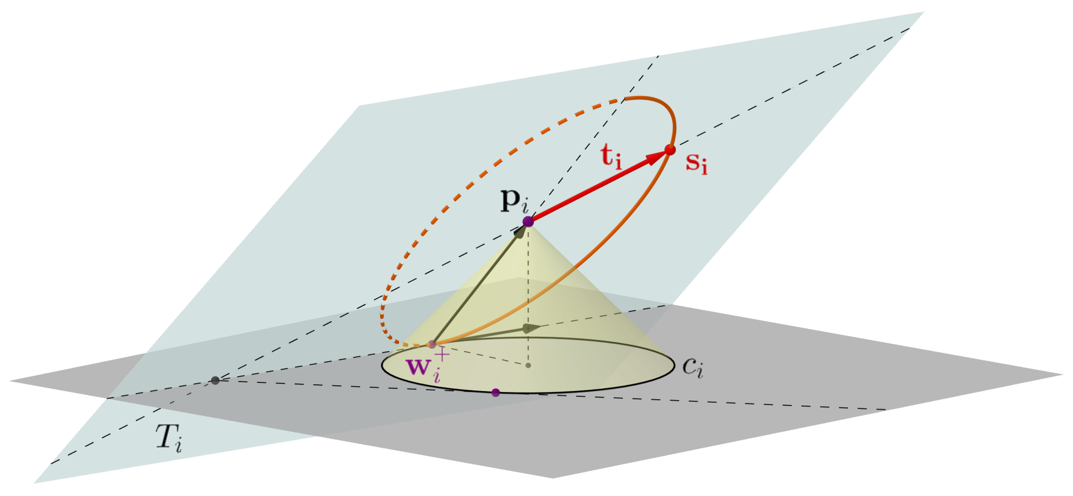
As a first step, let us determine the left touching point for each circle c i in C , and let us denote them by w i + ( i = 1 , 2 , , n ). Our aim is to reconstruct the tangent vector t i that if we substitute into (2), w i + = q i + holds. What we can observe is that there are infinitely many solutions. To geometrically construct the vector, let its starting point be p i . We can find the endpoints of appropriate tangent vectors on the plane T i that is tangent to the representing cone of p i (coming from the cyclographic representation) and that touches c i at w i + . In order to determine the endpoint s i of t i , we construct a circle which is on the plane T i and its center is p i . We define T i by the vectors
p i w i + , 0 and w i + p i , 0 .
The endpoint s i can be found along a semicircle of this circle. However, in practice, there is no specific need to use a circle; thus, we can cut the costs of normalizing the vectors (9). Consequently, we define s i along a semi-ellipse as follows:
s i = p i + cos u i p i x w i x + p i y w i y + p i z + sin u i w i y + p i y p i x w i x + 0 , u i 0 , π
Then, vector t i is given as s i p i ; thus, we can formulate it as
t i = cos u i p i x w i x + p i y w i y + p i z + sin u i w i y + p i y p i x w i x + 0 , u i 0 , π .
The approach is shown in Figure 2. Coming from the construction itself, it is guaranteed that the angle of t i and the x y -plane is less than π 4 , i.e., t i is always space-like.
Using the geometric interpretation of envelopes [12,13], we can obtain the other touching point easily as well. Let k i denote the line that goes through s i and p i . Then, w i can be determined using the other tangent to circle c i from the piercing point of k i . As the intersection line of T i and the x y -plane always touches the circle at w i + , and as the other touching point is determined using the other tangent line, it is proved that w i ± = q i ± .
This approach may be beneficial if the user would like to have more control of the final shape. By changing the value of u i in (11), the user is able to easily modify the position of w i . Moreover, as we will discuss in Section 4, it can be useful for eliminating intersections of the envelope curves.
Note that while in Kruppa’s method [22], the special case of w i + , w i , and p i being collinear has to be handled separately; our new method can handle all different situations uniformly. The collinearity happens when t i is parallel to the x y plane, but this is not a special case in the new method.
The method has its limitations as well. As opposed to the work in [22], as the position of the right touching point w i is not fixed, we cannot guarantee that it always lies outside the neighboring circles—however, it can be guaranteed for w i + .

3.2. Constructing the Envelope Curves

Now we have created the appropriate input set for circle set C = c 1 , c 2 , , c n , n N . That is, we obtained the set of spatial points P = { p 1 , p 2 , , p n } and the corresponding tangent vectors T = { t 1 , t 2 , , t n } to construct the envelope. We will then apply the RE curve interpolation algorithm [10] for each circle pair; therefore, for each pair of p i , t i , and p i + 1 , t i + 1 ( i = 1 , 2 , , n 1 ).
Technically, we may omit the first step of the algorithm (see Section 2.1) as we have already defined the touching points w i ± for each circle c i . We continue with the next step and construct the corresponding tangent vectors v i + and v i + 1 + for the touching points w i + and w i + 1 + . For this step, Bizzarri et al. leave the α i values as free parameters in (3). As Kruppa showed in [22], we may use the idea of Kunkli and Hoffmann [14] to define the corresponding tangent vectors based on the radical lines of the circles as follows:
v j = 2 d ( w j + , l i ) w j + p j w j + p j , j = i , i + 1 ,
where l i is the radical line of circles c i and c i + 1 , and d ( ) denotes the Euclidean distance. Then, we follow the remaining steps of the algorithm [10]. We construct the curve x i ( t ) interpolating w i + , w i + 1 + , v i , and v i + 1 , for example, using Hermite interpolation. To define the medial axis, we construct the polynomial function f i with the following boundary conditions, based on (5 and 6):
f i ( 0 ) = p i z v i , f i ( 1 ) = p i + 1 z v i + 1
and
f i ( 0 ) = t i · ( f i ( 0 ) x i ( 0 ) v i ) t i · v i , f i ( 1 ) = t i + 1 · ( f i ( 1 ) x i ( 1 ) v i + 1 ) t i + 1 · v i + 1 .
The function f i can be constructed in various ways, e.g., we may apply polynomial functions of degree 3 using Hermite interpolation. In the next section, we discuss how various choices of the function f i affect the shape of the envelope curves. The RE curve y i ( t ) is obtained as
y ¯ i ( t ) = y ( t ) , r ( t ) = x i x ( t ) + x i y ( t ) f i ( t ) , x i y ( t ) x i x ( t ) f i ( t ) , f i ( t ) x i x 2 ( t ) + x i y 2 ( t ) .
Finally, we apply the envelope formula [1] for y ¯ i , and we yield the x ± : [ a , b ] R 2 envelope curves as
x ± ( t ) = y ( t ) r ( t ) r ( t ) y ( t ) ± y ( t ) y ( t ) 2 r ( t ) 2 y ( t ) 2 .
As shown by Bizzarri et al. [10], y ¯ i is an RE curve and the x ± envelope curves are rational. To sum up, Algorithm 1 shows how we can apply the RE curve interpolation algorithm for circle skinning. As a result, we obtain a G 1 continuous spline of RE curves, while the yielded envelope curves also have G 1 continuity. Generally, our approach can be applied for any kind of MPH curve interpolation method using two endpoints and two tangent vectors.
Algorithm 1 A flexible approach for using RE/MPH curves for skinning purposes
Require: An admissible sequence of circles C = c 1 , c 2 , , c n
Ensure: The skinning curves as envelope curves with G 1 continuity
  1: w 1 ± = getByCommonTangentLines ( c 1 , c 2 )
  2: w n ± = getByCommonTangentLines ( c n 1 , c n )
  3: for i = 2 to n 1 do
  4:      w i ± = getFromApollonianSolutions ( c i 1 , c i , c i + 1 )
  5: for i = 1 to n do
  6:      p i = ( o i x , o i y , r i )
  7:      t i = getTVector ( p i , w i + )                   ▹ see (11)
  8: skin = { }
  9: for i = 1 to n 1 do
10:      v i = getV ( p i , w i + )
11:      v i + 1 = getV ( p i + 1 , w i + 1 + )                     ▹ see (12)
12:      x i ( t ) = interpolate ( w i + , w i + 1 + , v i , v i + 1 )
13:      f i ( t ) = getF ( p i , v i , t i , p i + 1 , v i + 1 , t i + 1 , x i )       ▹ see (13) and (14)
14:      y ¯ i ( t ) = getMAT ( x i , f i )                    ▹ see (15)
15:      x i ± ( t ) = getEnvelopeCurves ( y ¯ i )               ▹ see (16)
16:      skin . add ( x i ± )
17: return skin
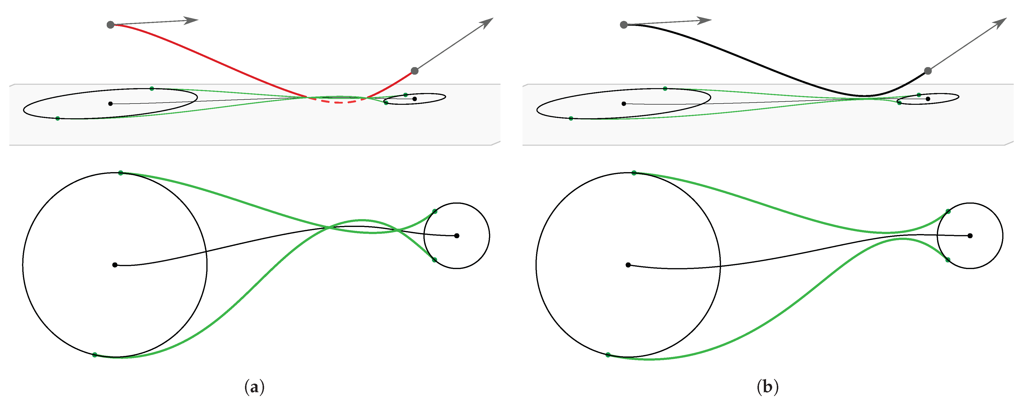
In Figure 3, we make a comparison between Kruppa’s approach [22] and our newly proposed method. In Figure 3a, two touching points are fixed on each circle and the right envelope curve intersects itself. In Figure 3b, we use our solution for the same input. Fixing the location of a single touching point gives the freedom to modify the final shape of the model, and we can eliminate the intersection. More complex models can be seen in Figure 4 that highlights the advantages of our proposed method.
Furthermore, from a practical point of view, our solution and Kruppa’s method [22] can be combined; thus, the user can decide for each circle separately whether to fix the location of only a single or both touching points. This combination of the methods provides the most efficient and flexible solution for the user.

4. Intersections of the Envelope Curves

In skinning, as generally in all types of modeling, we always strive for aesthetic results. One aspect can be to achieve visual smoothness [26], and another one is the lack of intersections. Now, we are focusing on intersections of the skinning curves with each other, and not on self-intersections of each curve. The detection of the intersections and computing the points of intersections is a challenging issue. There are many general approaches based on Bézier curves, for example, the subdivision scheme of the de Casteljau algorithm and clipping methods [27,28]. However, few studies have been carried out specifically for intersections of skinning curves. In [17], Kruppa et al. gave an algorithmic approach to resolve the intersections by modifying the tangent lengths of the Hermite interpolants.
In this section, we examine the detection and elimination of intersections of envelope curves in our specific case. For the admissible circle set C = c 1 , c 2 , , c n , n N , we examine the intersections of the envelope curves created for each circle pair c i and c i + 1 ( i = 1 , 2 , , n 1 ). For the sake of simpler notations, we will use y ¯ i , y i , x i , x i ± , and f i without indices, i.e., as y ¯ , y , x , x ± , and f.

4.1. Intersection Detection

Looking at the envelope curves, we can observe an interesting property for the y ¯ ( t ) curve considered as a MAT. If there exists a point of y ¯ ( t ) with the third coordinate being zero, then the envelope curves intersect each other at this exact point, and actually the MA and the MAT intersect each other at this point too. Moreover, the intersections happen at the same parameter value for each curve. Figure 5 shows an example to this property.
Moreover, examining the problem from an algebraic viewpoint, we can deduce that if y ¯ ( t ) has a tangent vector that is light-like, then the envelope curves will intersect each other at the corresponding parameter value. Based on these two observations, we can formalize the following theorem.
Theorem 1.
If y ¯ : [ a , b ] R 2 , 1 , y ¯ ( t ) = ( y ( t ) , r ( t ) ) is considered as the medial axis transform of a given planar domain, then its associated envelope curves x + ( t ) and x ( t ) intersect each other at a parameter value t j a , b (i.e., x + ( t j ) = x ( t j ) ), if and only if
  • r ( t j ) = 0 , or
  • y ¯ ( t j ) M = 0 , that is, the tangent vector of y ¯ at the parameter value t j is light-like.
Proof of Theorem 1.
If the envelope curves intersect each other at the parameter value t j , then x + ( t j ) = x ( t j ) has to hold ( t j a , b ). Based on (16), we can suppose that y ( t ) 0 , t a , b . We rewrite the x + ( t j ) = x ( t j ) equation into
r ( t j ) r ( t j ) y ( t j ) + y ( t j ) y ( t j ) 2 r ( t j ) 2 y ( t j ) 2 = r ( t j ) r ( t j ) y ( t j ) y ( t j ) y ( t j ) 2 r ( t j ) 2 y ( t j ) 2 .
Then, the following two cases arise:
  • If r ( t j ) = 0 , then x + ( t j ) = x ( t j ) = y ¯ ( t j ) = y ( t j ) .
  • If r ( t j ) 0 , then the equation can be written as
    y ( t j ) y ( t j ) 2 r ( t j ) 2 = y ( t j ) y ( t j ) 2 r ( t j ) 2 .
    Since y ( t j ) 0 , rearranging the equation we get
    y ( t j ) 2 r ( t j ) 2 = 0 ,
    thus, y ¯ ( t j ) M = 0 .
If r ( t j ) 0 and y ( t j ) 2 r ( t j ) 2 0 , then based on the above, x + ( t j ) x ( t j ) . Then, x + ( t j ) = x ( t j ) t j a , b if and only if r ( t j ) = 0 or y ¯ ( t j ) is light-like. □
Remark 1.
Theorem 1 can be also proved using a cyclographic approach.
  • If the third coordinate is zero for a point on the MAT, then it means that the radius of the corresponding cycle is zero. A cycle of zero radius is called null-cycle, and it is interpreted as a point. Moreover, the tangent lines drawn to this null-cycle touch it at the same point, thus this point becomes the point of the envelopes, i.e., x + ( t j ) = x ( t j ) .
  • If the tangent vector of the MAT at parameter value t j is light-like, then the tangent line at y ¯ ( t j ) is a generator line of the representing cone of y ¯ ( t j ) . In this case, the piercing point of the tangent line and the xy plane is a point on the cycle. As it is not possible to draw tangent lines from this point to the cycle, then the point of the envelope cannot be anything else than the point itself, so x + ( t j ) = x ( t j ) .
In all other cases, the touching points of a cycle always differ.
If we examine the intersections of the envelopes of RE/MPH curves specifically, then we obtain a special case of Theorem 1.
Corollary 1.
Given the y ¯ : 0 , 1 R 2 , 1 , y ¯ ( t ) = y ( t ) , r t = x x ( t ) + x y ( t ) f ( t ) , x y ( t ) x x ( t ) f ( t ) , f ( t ) x x 2 ( t ) + x x 2 ( t ) RE curve, the envelope curves x + , x : 0 , 1 R 2 intersect each other at a parameter value t j 0 , 1 (thus, x + ( t j ) = x ( t j ) ) if and only if
  • x ( t ) is irregular and x ( t j ) is a singular point;
  • x ( t ) is regular, but f ( t j ) = 0 holds; or
  • y ¯ ( t j ) M = 0 , i.e., the tangent vector of the RE curve at the parameter value t j is light-like.
Proof of Corollary 1.
The r ( t ) = f ( t ) x x 2 ( t ) + x x 2 ( t ) coordinate-function of the y ¯ RE curve is zero if and only if f ( t j ) = 0 or x x 2 ( t ) + x x 2 ( t ) = 0 , thus x ( t j ) = 0 . The third case of Corollary 1 is the second case of Theorem 1. □
Based on Corollary 1, to detect the points of intersections in the case of the RE curves, we need to find those t j parameter values for which x ( t j ) = 0 , f ( t j ) = 0 , or y ¯ ( t j ) M = 0 . The complexity of finding the singular points of x depends on the choice of x . If x is a cubic Hermite interpolant, then the equation x ( t j ) = 0 is quadratic. If x is regular, then the roots of the equation f ( t ) = 0 has to be found in the interval [ 0 , 1 ] . If f is a cubic polynomial, then the roots may be obtained even directly by the formula of Cardano. Looking at the third case of Corollary 1, the intersection points of the envelope curves can be obtained by solving y ( t j ) 2 r ( t j ) 2 = 0 .

4.2. Eliminating the Intersections

Now, we provide a method to eliminate the problem when there exist a parameter value t j [ 0 , 1 ] for which f ( t j ) = 0 ; thus, the envelope curves intersect each other (see Corollary 1). Let us assume that x is regular and the tangent vectors y ¯ ( t ) , t [ 0 , 1 ] are space-like. As f ( t j ) = 0 , x + ( t j ) = x ( t j ) . Our task is to achieve that f does not have any real roots in the interval [ 0 , 1 ] ; thus, the envelope curves do not intersect each other.
One solution is to fine-tune the parameter value u i in (11), which results in modifying the location of the touching point w i ; thus, the shape of the envelope curves changes too. We modify u i iteratively in the interval 0 , π until
f ( t ) > 0 , t 0 , 1
holds. This can be achieved in most cases as we have seen in practice; however, it is not guaranteed that we can find such a value. Figure 6 shows that by slightly modifying u i + 1 (and thus t i + 1 ) we achieved that the intersections are eliminated.
Another solution is modifying the function f itself. As shown in Section 2.2, f has to be constructed such that it satisfies the given boundary conditions. If f is created with Hermite interpolation yielding a polynomial function of degree 3, and it has real root(s) in the interval [ 0 , 1 ] , then we may increase its order. There exist infinitely many quartic polynomials that satisfy the given boundary conditions, and we need to choose one solution for which (17) holds. For this, let f be defined as
f ( t ) = t 4 + a 3 t 3 + a 2 t 2 + a 1 t + a 0
where
a 3 = f ˜ 0 + f ˜ 1 + f ˜ 0 2 f ˜ 1 2 k , a 2 = 3 f ˜ 1 3 f ˜ 0 2 f ˜ 0 f ˜ 1 + k , a 1 = f ˜ 0 , a 0 = f ˜ 0 ,
and f ˜ 0 , f ˜ 1 , f ˜ 0 , f ˜ 1 are the boundary conditions (5) and (6). In order to eliminate the intersections, we need to find such values for k R in (19) for which (17) holds. As f ( 0 ) and f ( 1 ) are always positive, f can always be constructed in a way that f ( t ) > 0 , t 0 , 1 —though it might be even higher in degree.
If f has a degree greater than three, then we obtain the intersection points by solving the equation f ( t ) = 0 using numerical methods, e.g., the Newton–Raphson method. Furthermore, as f can be written in a Bézier–Bernstein representation, we can specifically use Bézier clipping, which deals with finding the roots of a univariate polynomial function within a given interval in efficient ways [27,29,30,31,32,33].
Figure 7 shows that by increasing the degree of f ( t ) and choosing a suitable value for k, we eliminate the intersections. Note that neither the touching points, nor the tangent vectors have been changed, while the intersections are resolved.

5. Conclusions

In this work, we improved the method of applying RE and MPH curves for skinning purposes. As it was clear from the previous approach [22], choosing appropriate input data for the RE construction method [10] is critical to create the envelope curves of a discrete set of circles. We gave a new method by fixing the location of a single touching point on each circle, which gives more freedom for the user to modify the shape of the resulting envelope. Furthermore, we examined the crucial problem of unintentional intersections. As skinning is a modeling technique, the lack of intersections of the envelope curves is of utmost importance. We showed that a significant advantage of using MATs (and specifically RE and MPH curves) for skinning is the easy detection and elimination of intersections of the envelope curves. We provided a method to detect the intersection of envelope curves and gave two possible ways to eliminate the intersections. The discussed results greatly contribute towards the advantageous usage of RE and MPH curves in circle-based modeling.

Author Contributions

Conceptualization, K.K., R.K. and M.H.; methodology, K.K., R.K. and M.H.; software, K.K.; validation, K.K., R.K. and M.H.; investigation, K.K., R.K. and M.H.; writing—original draft preparation, K.K.; writing—review and editing, K.K., R.K. and M.H.; supervision, R.K. and M.H. All authors have read and agreed to the published version of the manuscript.

Funding

This work was supported by the construction EFOP-3.6.3-VEKOP-16-2017-00002. The project was supported by the European Union, co-financed by the European Social Fund.

Conflicts of Interest

The authors declare no conflict of interest. The funders had no role in the design of the study; in the collection, analyses, or interpretation of data; in the writing of the manuscript; or in the decision to publish the results.

References

  1. Moon, H.P. Minkowski Pythagorean hodographs. Comput. Aided Geom. Des. 1999, 16, 739–753. [Google Scholar] [CrossRef]
  2. Choi, H.I.; Choi, S.W.; Moon, H.P. Mathematical theory of medial axis transform. Pac. J. Math. 1997, 181, 57–88. [Google Scholar] [CrossRef]
  3. Choi, H.I.; Han, C.Y.; Moon, H.P.; Roh, K.H.; Wee, N.S. Medial axis transform and offset curves by Minkowski Pythagorean hodograph curves. Comput. Aided Des. 1999, 31, 59–72. [Google Scholar] [CrossRef]
  4. Kosinka, J.; Jüttler, B. G1 Hermite interpolation by Minkowski Pythagorean hodograph cubics. Comput. Aided Geom. Des. 2006, 23, 401–418. [Google Scholar] [CrossRef]
  5. Kosinka, J.; Šír, Z. C2 Hermite interpolation by Minkowski Pythagorean hodograph curves and medial axis transform approximation. Comput. Aided Geom. Des. 2010, 27, 631–643. [Google Scholar] [CrossRef]
  6. Kosinka, J.; Jüttler, B. C1 Hermite interpolation by Pythagorean hodograph quintics in Minkowski space. Adv. Comput. Math. 2009, 30, 123–140. [Google Scholar] [CrossRef]
  7. Bizzarri, M.; Lávička, M.; Vršek, J. Linear computational approach to interpolations with polynomial Minkowski Pythagorean hodograph curves. J. Comput. Appl. Math. 2019, 361, 283–294. [Google Scholar] [CrossRef]
  8. Kim, G.I.; Ahn, M.H. C1 Hermite interpolation using MPH quartic. Comput. Aided Geom. Des. 2003, 20, 469–492. [Google Scholar] [CrossRef]
  9. Kosinka, J.; Lávička, M. A unified Pythagorean hodograph approach to the medial axis transform and offset approximation. J. Comput. Appl. Math. 2011, 235, 3413–3424. [Google Scholar] [CrossRef] [Green Version]
  10. Bizzarri, M.; Lávička, M.; Kosinka, J. Medial axis transforms yielding rational envelopes. Comput. Aided Geom. Des. 2016, 46, 92–102. [Google Scholar] [CrossRef]
  11. Bizzarri, M.; Lávička, M.; Kosinka, J. Skinning and blending with rational envelope surfaces. Comput. Aided Des. 2017, 87, 41–51. [Google Scholar] [CrossRef] [Green Version]
  12. Peternell, M.; Odehnal, B.; Sampoli, M.L. On quadratic two-parameter families of spheres and their envelopes. Comput. Aided Geom. Des. 2008, 25, 342–355. [Google Scholar] [CrossRef] [Green Version]
  13. Pottmann, H.; Wallner, J. Computational Line Geometry; Springer: Berlin/Heidelberg, Germany, 2010. [Google Scholar]
  14. Kunkli, R.; Hoffmann, M. Skinning of circles and spheres. Comput. Aided Geom. Des. 2010, 27, 611–621. [Google Scholar] [CrossRef]
  15. Bastl, B.; Kosinka, J.; Lávička, M. Simple and branched skins of systems of circles and convex shapes. Graph. Model. 2015, 78, 1–9. [Google Scholar] [CrossRef]
  16. Bana, K.; Kruppa, K.; Kunkli, R.; Hoffmann, M. KSpheres—An efficient algorithm for joining skinning surfaces. Comput. Aided Geom. Des. 2014, 31, 499–509. [Google Scholar] [CrossRef] [Green Version]
  17. Kruppa, K.; Kunkli, R.; Hoffmann, M. An improved skinning algorithm for circles and spheres providing smooth transitions. Graph. Model. 2019, 101, 27–37. [Google Scholar] [CrossRef]
  18. Connolly, M.L. Analytical molecular surface calculation. J. Appl. Crystallogr. 1983, 16, 548–558. [Google Scholar] [CrossRef]
  19. Edelsbrunner, H. Deformable smooth surface design. Discret. Comput. Geom. 1999, 21, 87–115. [Google Scholar] [CrossRef] [Green Version]
  20. Rossignac, J.; Whited, B.; Slabaugh, G.; Fang, T.; Unal, G. Pearling: 3D interactive extraction of tubular structures from volumetric images. In Proceedings of the MICCAI Workshop on Interaction in Medical Image Analysis and Visualization, Brisbane, Australia, 29 October– 2 November 2007. [Google Scholar]
  21. Piskin, S.; Unal, G.; Arnaz, A.; Sarioglu, T.; Pekkan, K. Tetralogy of Fallot Surgical Repair: Shunt Configurations, Ductus Arteriosus and the Circle of Willis. Cardiovasc. Eng. Technol. 2017, 8, 107–119. [Google Scholar] [CrossRef] [PubMed] [Green Version]
  22. Kruppa, K. Applying Rational Envelope curves for skinning purposes. Front. Inf. Technol. Electron. Eng. 2021, 22, 202–209. [Google Scholar] [CrossRef]
  23. Farouki, R.T.; Sakkalis, T. Pythagorean hodographs. IBM J. Res. Dev. 1990, 34, 736–752. [Google Scholar] [CrossRef]
  24. Farouki, R.T.; Giannelli, C.; Sestini, A. New Developments in Theory, Algorithms, and Applications for Pythagorean-Hodograph Curves. In Advanced Methods for Geometric Modeling and Numerical Simulation; Giannelli, C., Speleers, H., Eds.; Springer International Publishing: Cham, Switzerland, 2019; pp. 127–177. [Google Scholar] [CrossRef]
  25. Bizzarri, M.; Lávička, M. Interpolation of Hermite data by clamped Minkowski Pythagorean hodograph B-spline curves. J. Comput. Appl. Math. 2021, 392. [Google Scholar] [CrossRef]
  26. Tornai, R. Measurement of visual smoothness of blending curves. Ann. Math. Inform. 2012, 40, 155–160. [Google Scholar]
  27. Sederberg, T.W.; Nishita, T. Curve intersection using Bézier clipping. Comput. Aided Des. 1990, 22, 538–549. [Google Scholar] [CrossRef]
  28. Lou, Q.; Liu, L. Curve intersection using hybrid clipping. Comput. Graph. 2012, 36, 309–320. [Google Scholar] [CrossRef]
  29. Bartoň, M.; Jüttler, B. Computing roots of polynomials by quadratic clipping. Comput. Aided Geom. Des. 2007, 24, 125–141. [Google Scholar] [CrossRef]
  30. Liu, L.; Zhang, L.; Lin, B.; Wang, G. Fast approach for computing roots of polynomials using cubic clipping. Comput. Aided Geom. Des. 2009, 26, 547–559. [Google Scholar] [CrossRef]
  31. Ko, K.H.; Kim, K. Improved subdivision scheme for the root computation of univariate polynomial equations. Appl. Math. Comput. 2013, 219, 7450–7464. [Google Scholar] [CrossRef]
  32. Chen, X.D.; Ma, W.; Ye, Y. A rational cubic clipping method for computing real roots of a polynomial. Comput. Aided Geom. Des. 2015, 38, 40–50. [Google Scholar] [CrossRef]
  33. Li, S.; Chen, G.; Wang, Y. An improved rational cubic clipping method for computing real roots of a polynomial. Appl. Math. Comput. 2019, 349, 207–213. [Google Scholar] [CrossRef]
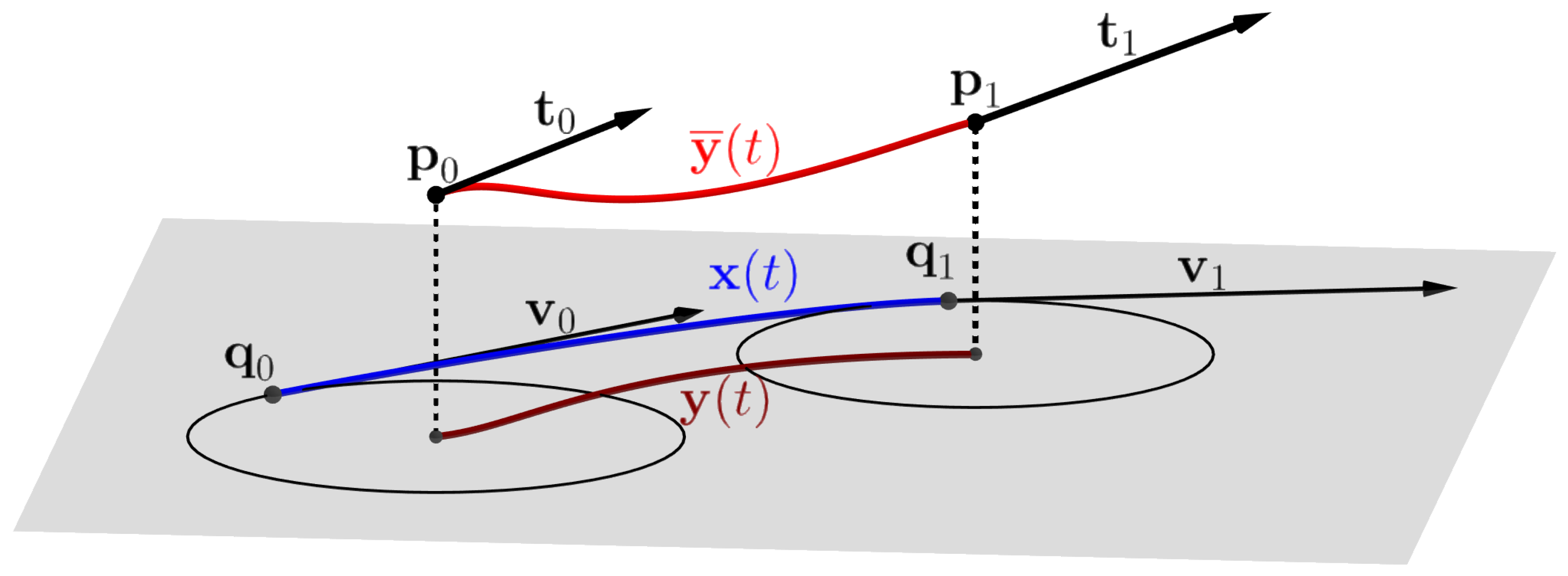
Figure 1. Constructing the RE curve y ¯ ( t ) for input data p 0 , p 1 , t 0 , and t 1 , using the method of Bizzarri et al. [10].
Mathematics 09 00843 g001
Figure 2. Computation of an appropriate tangent vector. We fix the location of the touching point w i + , which leaves the user the freedom to choose the endpoint of the tangent vector t i along a semi-ellipse.
Mathematics 09 00843 g002
Figure 3. (a) Fixing the location of two touching points on each circle, using the method of Kruppa [22]. (b) By fixing the location of a single touching point, we get more freedom to modify the shape of the envelope curves. It is possible that this way we eliminate certain self-intersections.
Mathematics 09 00843 g003
Figure 4. Comparison of the previous method [22] and our solution. (a) Snake model using the solution in [22]. (b) With our method, the unintended broader parts of the snake and intersections at the tail have been eliminated. (c) Crane bird model with the method in [22]. (d) By using our solution, we obtain the bill of the crane without intersections.
Mathematics 09 00843 g004
Figure 5. The envelope curves x + , x , the medial axis y , and the y ¯ medial axis transform intersect each other at the same point at the same parameter value.
Mathematics 09 00843 g005
Figure 6. (a) The envelope curves intersect each other. (b) By modifying the value of u i in (11), we obtain that f ( t ) > 0 ; thus, we resolve the intersections. With this solution, the location of one of the touching points on the second circle is changed.
Mathematics 09 00843 g006
Figure 7. (a) The envelope curves intersect because f ( t ) has real roots in the interval [ 0 , 1 ] . (b) If we increase the order of the function, then f ( t ) can be constructed in a way that we eliminate the intersection of the envelope curves. Note that the positions of the touching points do not change.
Mathematics 09 00843 g007
Publisher’s Note: MDPI stays neutral with regard to jurisdictional claims in published maps and institutional affiliations.