On the Simulation of a Special Class of Time-Inhomogeneous Diffusion Processes

Abstract

General methods to simulate probability density functions and first passage time densities are provided for time-inhomogeneous stochastic diffusion processes obtained via a composition of two Gauss–Markov processes conditioned on the same initial state. Many diffusion processes with time-dependent infinitesimal drift and infinitesimal variance are included in the considered class. For these processes, the transition probability density function is explicitly determined. Moreover, simulation procedures are applied to the diffusion processes obtained starting from Wiener and Ornstein–Uhlenbeck processes. Specific examples in which the infinitesimal moments include periodic functions are discussed.

1. Introduction

Time-inhomogeneous stochastic diffusion processes are often used to model real dynamic systems in various scientific areas as neurosciences, population dynamics, queueing systems, finance, and economics (cf., for instance, Buonocore et al. [1,2], Albano and Giorno [3], Giorno and Spina [4], Ricciardi et al. [5], Renshaw [6]), Di Crescenzo et al. [7], Linetsky [8], Glasserman [9]). Specifically, in Buonocore et al. [1,2], restricted Gauss–Markov processes are used to construct inhomogeneous leaky integrate-and-fire stochastic models for single neurons activity in the presence of a reversal hyperpolarization potential and time-varying input signals. In Albano and Giorno [3], a time-inhomogeneous Ornstein–Uhlenbeck is considered as a model for the membrane potential activity of a single neuron and a statistical procedure to fit the constant parameters and the time-dependent functions is proposed. Moreover, in Giorno and Spina [4], a time-inhomogeneous Ornstein–Uhlenbeck diffusion process with jumps is also analyzed. In Ricciardi et al. [5], special emphasis is put on neuronal firing problems and on the description of population dynamics, for which the first-passage time distribution and its statistics carry a fundamental relevance. In Renshaw [6], many aspects of population dynamics are covered, including Wiener and Ornstein–Uhlenbeck diffusion models and simulation techniques. In Di Crescenzo et al. [7], the authors derive a heavy-traffic approximation that allows for approximating the state of the systems by a time-non-homogeneous Wiener process subject to jumps due to catastrophes and random returns to the zero state due to repairs. In Linetsky [8], explicit analytical expressions for transition densities of Brownian motion with drift, the Ornstein–Uhlenbeck process, and affine (square-root) diffusion with one or two reflecting barriers are obtained in the context of economics and finance. In Glasserman [9], the Monte Carlo simulation plays an essential tool in the pricing of derivative securities and in risk management.

To include several aspects of the real phenomena, one is led to consider increasing complex processes (cf., for instance, Di Crescenzo et al. [10], Giorno et al. [11,12], Abundo [13], Veestraeten [14], Molini et al. [15], Lim and Muniandy [16], Jeon et al. [17]). In these contexts, the focus is on specific probabilistic characteristics that define the behavior of the stochastic processes as the transition distributions and the related moments as well as the first passage time through specific time-dependent boundaries. In particular, in Di Crescenzo et al. [10], and in Giorno et al. [11,12], new procedures for constructing transition probability density functions and first passage time densities through constant boundaries are proposed for generally time-inhomogeneous diffusion processes. In Abundo [13], some asymptotic results for diffusions and Gauss–Markov process and their fractional integrals are obtained. In Veestraeten [14], the transition and first hitting time densities and moments for the Ornstein–Uhlenbeck process between exponential thresholds are derived. Moreover, in Molini et al. [15], first passage time statistics, such as the survival probabilities and first passage time densities, are obtained analytically for the Brownian motion driven by time-dependent drift and diffusion coefficients. In Lim and Muniandy [16] and Jeon et al. [17], some Gaussian models for anomalous diffusion are considered, and the first passage time problem is discussed. These processes are used to model physical and biological systems.

Moreover, various efforts are direct to computational approaches (Di Nardo et al. [18], Taillefumier and Magnasco [19], D’Onofrio and Pirozzi [20]) that also involve methods of statistical inferences (Albano et al. [21], Albano and Giorno [22], Ramos-Ábalos et al. [23]). Specifically, in Di Nardo et al. [18] and Taillefumier and Magnasco [19] methods to construct first-passage-time probability density functions for Gauss–Markov processes through time-dependent boundaries are proposed. In D’Onofrio and Pirozzi [20], the problem of escape times from a region confined by two time-dependent boundaries is considered for a class of Gauss–Markov processes. Moreover, numerical procedures to infer the models based on time-inhomogeneous diffusion processes are proposed in Albano et al. [21], Albano and Giorno [22], and Ramos-Ábalos et al. [23].

However, sometimes these strategies are not actionable or not convenient and an approach based on the simulation of the processes is required (see, for instance, Buonocore et al. [24,25], Tuerlinckx et al. [26], Di Crescenzo et al. [27], Giraudo et al. [28], Herrann and Zucca [29], Headrick and Mugdadi [30], Devroye [31], Iacus [32]). In particular, in Buonocore et al. [24,25], algorithms for the simulation of sample paths and to generate random variates from probability density function of Gauss–Markov processes, restricted by particular time-dependent reflecting boundaries, are proposed. Furthermore, in Tuerlinckx et al. [26], some methods for the simulation of the Wiener process with constant drift and variance are described and compared on two criteria: simulation speed and accuracy of the simulation. In Di Crescenzo et al. [27], Giraudo et al. [28] and Herrann and Zucca [29], simulation procedures to estimate first-passage-time densities are constructed. Moreover, in Headrick and Mugdadi [30], algorithms for extending the class of generalized lambda distributions from univariate to multivariate data generation are presented. Finally, Iacus [32] focuses on the simulation and inference for general stochastic differential equations.

Random variates generation is a fundamental aspect of simulation modeling and analysis (cf., for instance, Devroye [31]). Indeed, in real applications, the distribution of a function of more iid (independent and identically distributed) random variables (statistics, estimators) is often computed via the simulation only, when the resulting distribution can not be deduced analytically. For this purpose, it is necessary to identify suitable methods to simulate the single random variable of interest. Standard procedures, as the inverse transformation method and the acceptance-rejection technique, often cannot be applied successfully so that ad hoc methods are needed to generate a sample of observations and then plot the resulting empirical histogram that can be compared with the related known probability density. The knowledge of effective simulation methods for single random variates generation allows for obtaining the histogram of the distribution of the statistics and the estimators that often have analytically non-computable distributions.

In Giorno and Nobile [33], a special class of time-inhomogeneous diffusion processes is defined and analyzed. These processes are obtained by using the composition of two Gauss–Markov processes conditioned to start from the same initial state. They are useful to model dynamical systems that switch randomly between two different regimes. This class includes diffusion processes with time-dependent infinitesimal moments for which the transition probability density function (pdf) is a mixture of two normal densities with weights depending on the initial condition and on a real parameter $\vartheta \in [0,1]$. General methods to analyze the first-passage time (FPT) are given, and FPT densities are explicitly obtained for suitable time-varying boundaries.

In the present paper, we propose theoretical and computational approaches based on the simulation to investigate on the transition densities, on the related conditional moments and on the FPT densities for the diffusion processes considered in [33].

The paper is organized as follows. In Section 2, starting from two Gauss Markov processes conditioned on the same initial state, we construct a continuous process $Y\left(t\right)$ by using the composition method. We formulate an algorithm to obtain the simulated density and a procedure for the simulation of the sample paths of $Y\left(t\right)$. In Section 3, we focus on a class of time-inhomogeneous diffusion processes $Z\left(t\right)$, whose transition pdf identifies with the density of $Y\left(t\right)$. In particular, for $\vartheta =0$ and $\vartheta =1$, one has $Z\left(t\right)=Y\left(t\right)$ for all t, so that an algorithm to simulate the FPT through a general time-dependent boundary is formulated. Furthermore, we show that such algorithm can be generalized to the case $0<\vartheta <1$. In Section 4 and Section 5, we apply the theoretical results and the proposed algorithms to diffusion processes obtained by the composition of Wiener processes and Ornstein–Uhlenbeck processes, respectively, by using the statistical environment and the language R. In both these cases, for fixed time instants, we simulate the random variable describing $Y\left(t\right)$, and we show that the transition pdf of the related diffusion process $Z\left(t\right)$ can be superimposed over the histogram of the process $Y\left(t\right)$ obtained via the simulation method. Moreover, for $\vartheta =0$ and $\vartheta =1$, making use of the simulation of the sample-paths, we obtain the histogram of first passage times of $Z\left(t\right)$ through time-dependent boundaries. Finally, the histogram of first passage times is compared with the closed form FPT density through special boundaries.

2. Composition Method for Gauss–Markov Processes

Let $m\left(t\right),h_1\left(t\right),h_2\left(t\right)$ be $C^1\left(T\right)$-class functions, where $C^1\left(T\right)$ denotes the set of continuously differentiable functions on T, with a T continuous parameter set, such that $h_2\left(t\right)\ne 0$ and $r\left(t\right)=h_1\left(t\right)/h_2\left(t\right)$ is a non-negative and monotonically increasing function. Let $\{X_i\left(t\right),t\ge \tau \}$ be the Gauss–Markov processes conditioned to start from y at time $\tau$ (see, Mehr and McFadden [34]):

$$\begin{array}{ccc}& & X_i\left(t\right)={(-1)}^{3-i}m\left(t\right)+\left[y-{(-1)}^{3-i}m\left(\tau \right)\right]\frac{h_2\left(t\right)}{h_2\left(\tau \right)}+h_2\left(t\right)W[r\left(t\right)-r\left(\tau \right)]\hfill \\ & & (i=1,2;t\ge \tau ;t,\tau \in T;y\in \mathbb{R}),\hfill \end{array}$$

(1)

where $\left\{W\right(t),t\ge 0\}$ is a standard Wiener process. The pdf $f_{X_i}(x,t)$ of $X_i\left(t\right)$$(i=1,2)$ is the normal density

$$f_{X_i}(x,t)=\frac{1}{\sqrt{2\pi V\left(t\right|\tau )}}exp\left\{-\frac{{[x-M_i\left(t\right|y,\tau )]}^2}{2V\left(t\right|\tau )}\right\},x\in \mathbb{R},t\ge \tau ,$$

(2)

with mean and variance

$$\begin{array}{cc}\hfill & E\left[X_i\left(t\right)\right]=M_i\left(t\right|y,\tau )={(-1)}^{3-i}m\left(t\right)+\frac{h_2\left(t\right)}{h_2\left(\tau \right)}\left[y-{(-1)}^{3-i}m\left(\tau \right)\right],\hfill \\ \hfill & \mathrm{Var}\left[X_i\left(t\right)\right]=V\left(t\right|\tau )=h_2\left(t\right)\left[h_1\left(t\right)-\frac{h_2\left(t\right)}{h_2\left(\tau \right)}{h}_1\left(\tau \right)\right].\hfill \end{array}$$

(3)

Starting from the Gauss–Markov processes $X_1\left(t\right)$ and $X_2\left(t\right)$, conditioned to start from y at time $\tau$, we use the composition method (cf., for instance, Ross [35]) to construct a new stochastic process $\left\{Y\right(t),t\ge \tau \}$.

Let $0\le \vartheta \le 1$ be a real number and let $X_1\left(t\right)$ and $X_2\left(t\right)$ be the Gauss–Markov processes conditioned to start from y at time $\tau$, defined in (1). For any fixed $t\in T$, we assume that $U_{y,\tau }\left(t\right)$ is a random variable uniform in $(0,1)$, independent of $X_1\left(t\right)$ and $X_2\left(t\right)$. Then, the stochastic process $\left\{Y\right(t),t\ge \tau \}$, defined as

$$Y\left(t\right)=\left\{\begin{array}{cc}{\displaystyle X_1\left(t\right),}\hfill & 0\le U_{y,\tau }\left(t\right)<Q_{y,\tau }\left(\vartheta \right),\hfill \\ \hfill \\ {\displaystyle X_2\left(t\right),}\hfill & Q_{y,\tau }\left(\vartheta \right)\le U_{y,\tau }\left(t\right)<1,\hfill \end{array}\right.$$

(4)

with

$$Q_{y,\tau }\left(\vartheta \right)=\frac{\vartheta }{\vartheta +(1-\vartheta )exp\left\{-\frac{2m\left(\tau \right)}{v\left(\tau \right)}y\right\}},$$

(5)

where $v\left(t\right)=h_1\left(t\right)h_2\left(t\right)$, is characterized by pdf

$$f_Y(x,t)=Q_{y,\tau }\left(\vartheta \right)f_{X_1}(x,t)+\left[1-Q_{y,\tau }\left(\vartheta \right)\right]f_{X_2}(x,t),x\in \mathbb{R},t\ge \tau .$$

(6)

The density $f_Y(x,t)$ in (6) is a mixture, or a composition, of the two normal densities $f_{X_1}(x,t)$ and $f_{X_2}(x,t)$, with means and variances given in (3). In particular, by virtue of (4) and (6), we note that $Y\left(t\right)=X_2\left(t\right)$ and $f_Y(x,t)=f_{X_2}(x,t)$ when $\vartheta =0$, whereas $Y\left(t\right)=X_1\left(t\right)$ and $f_Y(x,t)=f_{X_1}(x,t)$ when $\vartheta =1$.

In the following, we formulate an algorithm to generate random variates from the pdf (6) by using the stochastic equations (1) and the composition method (4). Furthermore, we derive an algorithm for the simulation of the sample paths of $Y\left(t\right)$ via the composition method.

2.1. Simulated Pdf of the Process $Y\left(t\right)$

Let $t\in T$ be a fixed instant and $(y,\tau )\in \mathbb{R}\times T$ fixed real constants. For $t\ge \tau$, we obtain a random sample of N observations of $Y\left(t\right)$, and we construct the histogram of the random sample with the density (6) as a function of x.

We first note that $W\left[r\right(t)-r(\tau \left)\right]$ in (1) is characterized by a normal distribution with zero mean and variance $r\left(t\right)-r\left(\tau \right)$, so that we can write $W[r\left(t\right)-r\left(\tau \right)]=\sqrt{r\left(t\right)-r\left(\tau \right)}{\xi }_{\tau ,t}$, with ${\xi }_{\tau ,t}\sim \mathcal{N}(0,1)$. Hence, we formulate the following:

Algorithm 1

Let $(y,\tau )\in \mathbb{R}\times T$ be fixed real constants and $t\in T$ be a fixed instant such that $t\ge \tau$. Step 1: Generate ${\xi }_{\tau ,t}\sim \mathcal{N}(0,1)$ and $U_{y,\tau }\left(t\right)\sim \mathcal{U}(0,1)$, with $U_{y,\tau }\left(t\right)$ and ${\xi }_{\tau ,t}$ independent random numbers; Step 2: From (1), generate $X_i\left(t\right)$ as $$\begin{array}{ccc}& & X_i\left(t\right)={(-1)}^{3-i}m\left(t\right)+\left[y-{(-1)}^{3-i}m\left(\tau \right)\right]\frac{h_2\left(t\right)}{h_2\left(\tau \right)}+h_2\left(t\right)\sqrt{r\left(t\right)-r\left(\tau \right)}{\xi }_{\tau ,t}\hfill \\ & & (i=1,2;t\ge \tau );\hfill \end{array}$$ (7) Step 3: Making use of (7), generate $Y\left(t\right)$ via (4); Step 4: Repeat Steps 1 and 2 for N times, obtaining a random sample of size N from the density (6). The simulated pdf is then depicted by means of a histogram as function of x. The related sample moments can also be obtained.

2.2. Simulation of the Sample Paths of $Y\left(t\right)$

We first generate the sample paths of the Gauss–Markov processes $X_1\left(t\right)$ and $X_2\left(t\right)$, according to the stochastic equations (1) by using an exact simulation method (cf., for instance, Kroese et al. [36]).

Let s and t be time instants, such that $\tau <s<t$; by virtue of (1), we obtain:

$$\begin{array}{ccc}& & X_i\left(t\right)-X_i\left(s\right)\frac{h_2\left(t\right)}{h_2\left(s\right)}={(-1)}^{3-i}m\left(t\right)-{(-1)}^{3-i}m\left(s\right)\frac{h_2\left(t\right)}{h_2\left(s\right)}\hfill \\ & & +h_2\left(t\right)\left\{W\left[r\right(t)-r(\tau \left)\right]-W\left[r\right(s)-r(\tau \left)\right]\right\}(i=1,2).\hfill \end{array}$$

(8)

Since $W[r\left(t\right)-r\left(\tau \right)]-W[r\left(s\right)-r\left(\tau \right)]=\sqrt{r\left(t\right)-r\left(s\right)}{\xi }_{s,t}$, with ${\xi }_{s,t}\sim \mathcal{N}(0,1)$, for $\tau <s<t$ from (8), one has:

$$\begin{array}{ccc}& & X_i\left(t\right)={(-1)}^{3-i}m\left(t\right)+\frac{h_2\left(t\right)}{h_2\left(s\right)}\left[X_i\left(s\right)-{(-1)}^{3-i}m\left(s\right)\right]\hfill \\ & & +h_2\left(t\right)\sqrt{r\left(t\right)-r\left(s\right)}{\xi }_{s,t},(i=1,2).\hfill \end{array}$$

(9)

For the process $Y\left(t\right)$, from (4), one obtains:

$$Y\left(t\right)=Y\left(s\right)\frac{h_2\left(t\right)}{h_2\left(s\right)}+R_{y,\tau }(s,t)+h_2\left(t\right)\sqrt{r\left(t\right)-r\left(s\right)}{\xi }_{s,t}(\tau <s<t),$$

(10)

where

$$R_{y,\tau }(s,t)=\left\{\begin{array}{c}m\left(t\right)-m\left(s\right)\frac{h_2\left(t\right)}{h_2\left(s\right)},\hfill \\ 0\le U_{y,\tau }\left(s\right)<Q_{y,\tau }\left(\vartheta \right),0\le U_{y,\tau }\left(t\right)<Q_{y,\tau }\left(\vartheta \right),\hfill \\ \\ m\left(t\right)+m\left(s\right)\frac{h_2\left(t\right)}{h_2\left(s\right)}-2\frac{h_2\left(t\right)}{h_2\left(\tau \right)}m\left(\tau \right),\hfill \\ Q_{y,\tau }\left(\vartheta \right)\le U_{y,\tau }\left(s\right)<1,0\le U_{y,\tau }\left(t\right)<Q_{y,\tau }\left(\vartheta \right),\hfill \\ \\ -m\left(t\right)-m\left(s\right)\frac{h_2\left(t\right)}{h_2\left(s\right)}+2\frac{h_2\left(t\right)}{h_2\left(\tau \right)}m\left(\tau \right),\hfill \\ 0\le U_{y,\tau }\left(s\right)<Q_{y,\tau }\left(\vartheta \right),Q_{y,\tau }\left(\vartheta \right)\le U_{y,\tau }\left(t\right)<1,\hfill \\ \\ -m\left(t\right)+m\left(s\right)\frac{h_2\left(t\right)}{h_2\left(s\right)},\hfill \\ Q_{y,\tau }\left(\vartheta \right)\le U_{y,\tau }\left(s\right)<1,Q_{y,\tau }\left(\vartheta \right)\le U_{y,\tau }\left(t\right)<1.\hfill \end{array}\right.$$

(11)

Then, the following algorithm can be implemented:

Algorithm 2

Let $t_1<t_2<\dots <t_n$, with $t_k=\tau +(k-1)h$$(h>0,k=1,2\dots ,n)$, be the set of equidistant time instants for which the simulation of $Y\left(t\right)$ is required. Step 1: Set $t_1=\tau$ and $Y\left(t_1\right)=Y\left(\tau \right)=y$; Step 2: For $k=2,3,\dots ,n$ set $$Y\left(t_k\right)=Y\left(t_{k-1}\right)\frac{h_2\left(t_k\right)}{h_2\left(t_{k-1}\right)}+R_{y,\tau }(t_{k-1},t_k)+h_2\left(t\right)\sqrt{r\left(t_k\right)-r\left(t_{k-1}\right)}{\xi }_k,$$ (12) where ${\xi }_1,{\xi }_2,\dots ,{\xi }_n$$\stackrel{iid}{=}$$\mathcal{N}(0,1)$ and $$R_{y,\tau }(t_{k-1},t_k)=\left\{\begin{array}{c}m\left(t_k\right)-m\left(t_{k-1}\right)\frac{h_2\left(t_k\right)}{h_2\left(t_{k-1}\right)},\hfill \\ 0\le U_{k-1}<Q_{y,\tau }\left(\vartheta \right),0\le V_k<Q_{y,\tau }\left(\vartheta \right),\hfill \\ \\ m\left(t_k\right)+m\left(t_{k-1}\right)\frac{h_2\left(t_k\right)}{h_2\left(t_{k-1}\right)}-2\frac{h_2\left(t_k\right)}{h_2\left(\tau \right)}m\left(\tau \right),\hfill \\ Q_{y,\tau }\left(\vartheta \right)\le U_{k-1}<1,0\le V_k<Q_{y,\tau }\left(\vartheta \right),\hfill \\ \\ -m\left(t_k\right)-m\left(t_{k-1}\right)\frac{h_2\left(t_k\right)}{h_2\left(t_{k-1}\right)}+2\frac{h_2\left(t_k\right)}{h_2\left(\tau \right)}m\left(\tau \right),\hfill \\ 0\le U_{k-1}<Q_{y,\tau }\left(\vartheta \right),Q_{y,\tau }\left(\vartheta \right)\le V_k<1,\hfill \\ \\ -m\left(t_k\right)+m\left(t_{k-1}\right)\frac{h_2\left(t_k\right)}{h_2\left(t_{k-1}\right)},\hfill \\ Q_{y,\tau }\left(\vartheta \right)\le U_{k-1}<1,Q_{y,\tau }\left(\vartheta \right)\le V_k<1,\hfill \end{array}\right.$$ (13) with $U_1,U_2,\dots ,U_n$$\stackrel{iid}{=}$$\mathcal{U}(0,1)$ and $V_1,V_2,\dots ,V_n$$\stackrel{iid}{=}$$\mathcal{U}(0,1)$, being $U_1,U_2,\dots ,U_n$, $V_1,V_2,\dots ,V_n$ and ${\xi }_1,{\xi }_2,\dots ,{\xi }_n$ independent random numbers.

Formula (12) is a stochastic recurrence equation: starting from $Y\left(\tau \right)=y$ that is assumed to be known, it produces a sample path for $Y\left(t\right)$ at the desired times $t_1,t_2,\dots ,t_n$.

3. Some Time-Inhomogeneous Diffusion Processes

Let $\left\{Z\right(t),t\in T\}$ be a time-inhomogeneous diffusion process with infinitesimal drift and infinitesimal variance

$$\begin{array}{cc}\hfill & B_1(x,t)=\frac{h_2^{\prime }\left(t\right)}{h_2\left(t\right)}x+\left[m^{\prime }\left(t\right)-\frac{h_2^{\prime }\left(t\right)}{h_2\left(t\right)}m\left(t\right)\right]\frac{\vartheta -(1-\vartheta )exp\left\{-\frac{2m\left(t\right)}{v\left(t\right)}x\right\}}{\vartheta +(1-\vartheta )exp\left\{-\frac{2m\left(t\right)}{v\left(t\right)}x\right\}},x\in \mathbb{R},\hfill \\ \hfill & B_2\left(t\right)=h_2^2\left(t\right)r^{\prime }\left(t\right),\hfill \end{array}$$

(14)

where $0\le \vartheta \le 1$ is a real number and $m\left(t\right),h_1\left(t\right),h_2\left(t\right),v\left(t\right)$ are chosen as in Section 2. As proved in Giorno and Nobile [33], if one of the following assumptions is satisfied:

(a) 

the left endpoint of T is zero, $(y,\tau )=(0,0)$, $m\left(\tau \right)=h_1\left(\tau \right)=0$;

(b) 

$m\left(t\right)=c{h}_1\left(t\right),t\in T,c\in \mathbb{R}$,

The density (6) identifies with the transition pdf $f(x,t|y,\tau )=\partial P\{Z\left(t\right)\le x\left|Z\right(\tau )=y\}/\partial x$ of the diffusion process $Z\left(t\right)$. Then, in the cases (a) and (b), for all fixed $t\ge \tau$, one has $Z\left(t\right)\stackrel{d}{=}Y\left(t\right)$.

3.1. Case (a)

If the left endpoint of T is zero, $(y,\tau )=(0,0)$, $m\left(\tau \right)=h_1\left(\tau \right)=0$, the transition pdf of the diffusion process $Z\left(t\right)$, with infinitesimal moments (14), is:

$$\begin{array}{cc}& f_Z(x,t|0,0)=\left[\vartheta +(1-\vartheta )exp\left\{-\frac{2m\left(t\right)}{v\left(t\right)}x\right\}\right]\frac{1}{\sqrt{2\pi v\left(t\right)}}exp\left\{-\frac{{[x-m\left(t\right)]}^2}{2v\left(t\right)}\right\}\\ & (x\in \mathbb{R}),\end{array}$$

(15)

and the conditional mean and variance are:

$$\begin{array}{cc}\hfill E\left[Z\right(t\left)\right|Z\left(0\right)=0|& =(2\vartheta -1)m\left(t\right),\hfill \\ \hfill \mathrm{Var}\left[Z\right(t\left)\right|Z\left(0\right)=0]& =v\left(t\right)+4\vartheta (1-\vartheta )m^2\left(t\right),\hfill \end{array}$$

(16)

respectively.

3.2. Case (b)

If $m\left(t\right)=c{h}_1\left(t\right)$ for $t\in T$ and $c\in \mathbb{R}$, the infinitesimal moments (14) of $Z\left(t\right)$ become:

$$\begin{array}{cc}\hfill & B_1(x,t)=\frac{h_2^{\prime }\left(t\right)}{h_2\left(t\right)}x+\frac{c{B}_2\left(t\right)}{h_2\left(t\right)}\frac{\vartheta -(1-\vartheta )exp\left\{-\frac{2c}{h_2\left(t\right)}x\right\}}{\vartheta +(1-\vartheta )exp\left\{-\frac{2c}{h_2\left(t\right)}x\right\}},x\in \mathbb{R}\hfill \\ \hfill & B_2\left(t\right)=h_2^2\left(t\right)r^{\prime }\left(t\right),\hfill \end{array}$$

(17)

and, from (6), one obtains the transition pdf:

$$\begin{array}{ccc}& & f_Z(x,t|y,\tau )=\frac{\vartheta +(1-\vartheta )exp\left\{-\frac{2c}{h_2\left(t\right)}x\right\}}{\vartheta +(1-\vartheta )exp\left\{-\frac{2c}{h_2\left(\tau \right)}y\right\}}\frac{1}{\sqrt{2\pi V\left(t\right|\tau )}}exp\left\{-\frac{{[x-M_1\left(t\right|y,\tau )]}^2}{2V\left(t\right|\tau )}\right\},\hfill \\ & & (x\in \mathbb{R}),\hfill \end{array}$$

(18)

where $M_1\left(t\right|y,\tau )$ and $V\left(t\right|\tau )$ are given in (3), with $m\left(t\right)=c{h}_1\left(t\right)$. Then, the conditional mean and the variance of $Z\left(t\right)$ are:

$$\begin{array}{cc}\hfill E\left[Z\right(t\left)\right|Z\left(\tau \right)=y|& =\frac{h_2\left(t\right)}{h_2\left(\tau \right)}y+\frac{cV\left(t\right|\tau )}{h_2\left(t\right)}\frac{\vartheta -(1-\vartheta )exp\left\{-\frac{2c}{h_2\left(\tau \right)}y\right\}}{\vartheta +(1-\vartheta )exp\left\{-\frac{2c}{h_2\left(\tau \right)}y\right\}},\hfill \\ \hfill \mathrm{Var}\left[Z\right(t\left)\right|Z\left(\tau \right)=y]& =V\left(t\right|\tau )+{\left[\frac{cV\left(t\right|\tau )}{h_2\left(t\right)}\right]}^2\frac{4\vartheta (1-\vartheta )exp\left\{-\frac{2c}{h_2\left(\tau \right)}y\right\}}{{\left[\vartheta +(1-\vartheta )exp\left\{-\frac{2c}{h_2\left(\tau \right)}y\right\}\right]}^2}·\hfill \end{array}$$

(19)

Furthermore, for the time-inhomogeneous diffusion process defined in (14), let

$${\mathcal{T}}_Z=\left\{\begin{array}{c}\underset{t\ge \tau }{inf}\{t:Z\left(t\right)\ge S\left(t\right)\},Z\left(\tau \right)=y<S\left(\tau \right),\hfill \\ \tau ,t\in T\hfill \\ \underset{t\ge \tau }{inf}\{t:Z\left(t\right)\le S\left(t\right)\},Z\left(\tau \right)=y>S\left(\tau \right),\hfill \end{array}\right.$$

(20)

be the FPT of $Z\left(t\right)$ from $Z\left(\tau \right)=y$ to the boundary $S\left(t\right)\in C^1\left(T\right)$ and let $g_Z[S\left(t\right),t|y,\tau ]=\partial P({\mathcal{T}}_Z\le t)/\partial t$ be the FPT pdf, with $y\ne S\left(\tau \right)$. The FPT pdf $g_Z[S\left(t\right),t|y,\tau ]$ is a solution of the first-kind Volterra integral equation:

$$\begin{array}{ccc}& & f_Z(x,t|y,\tau )={\int }_{\tau }^t{g}_Z[S\left(u\right),u|y,\tau ]f_Z[x,t|S\left(u\right),u]du,\hfill \\ & & [y<S(\tau ),x\ge S(t\left)\right]\mathrm{or}[y>S(\tau ),x\le S(t\left)\right].\hfill \end{array}$$

(21)

Making use of (18) in (21), one obtains:

$$\begin{array}{ccc}& & g_Z[S\left(t\right),t|y,\tau ]=\frac{\vartheta +(1-\vartheta )exp\left\{-\frac{2c}{h_2\left(t\right)}S\left(t\right)\right\}}{\vartheta +(1-\vartheta )exp\left\{-\frac{2c}{h_2\left(\tau \right)}y\right\}}{g}_{X_1}[S\left(t\right),t|y,\tau ],\hfill \\ & & [y<S(\tau \left)\right]\mathrm{or}[y>S(\tau \left)\right].\hfill \end{array}$$

(22)

Similarly, the FPT densities of the processes $X_1\left(t\right)$ and $X_2\left(t\right)$ are also solutions of first-kind Volterra integral equations:

$$\begin{array}{ccc}& & f_{X_i}(x,t|y,\tau )={\int }_{\tau }^t{g}_{X_i}[S\left(u\right),u|y,\tau ]f_{X_i}[x,t|S\left(u\right),u]du(i=1,2),\hfill \\ & & [y<S(\tau ),x\ge S(t\left)\right]\mathrm{or}[y>S(\tau ),x\le S(t\left)\right].\hfill \end{array}$$

(23)

In the case (b), the transition densities of the processes $X_1\left(t\right)$ and $X_2\left(t\right)$ satisfy the following symmetry relation:

$$f_{X_2}(x,t|y,\tau )=exp\left\{-\frac{2c}{h_2\left(t\right)}x\right\}exp\left\{\frac{2c}{h_2\left(\tau \right)}y\right\}{f}_{X_1}(x,t|y,\tau ),$$

so that, from (23), one has:

$$g_{X_1}[S\left(t\right),t|y,\tau ]=exp\left\{\frac{2c}{h_2\left(t\right)}S\left(t\right)\right\}exp\left\{-\frac{2c}{h_2\left(\tau \right)}y\right\}{g}_{X_2}[S\left(t\right),t|y,\tau ].$$

(24)

Hence, for the diffusion process $Z\left(t\right)$ with infinitesimal moments (17), from (22) and (24), one obtains

$$\begin{array}{ccc}& & g_Z[S\left(t\right),t|y,\tau ]=Q_{y,\tau }\left(\vartheta \right)g_{X_1}[S\left(t\right),t|y,\tau ]+[1-Q_{y,\tau }\left(\vartheta \right)]g_{X_2}[S\left(t\right),t|y,\tau ]\hfill \\ & & [y<S(\tau ),x\ge S(t\left)\right]\mathrm{or}[y>S(\tau ),x\le S(t\left)\right],\hfill \end{array}$$

(25)

where $0\le \vartheta \le 1$,

$$Q_{y,\tau }\left(\vartheta \right)=\frac{\vartheta }{\vartheta +(1-\vartheta )exp\left\{-\frac{2c}{h_2\left(\tau \right)}y\right\}}$$

and $g_{X_i}[S\left(t\right),t|y,\tau ]$ denotes the FPT density of $X_i\left(t\right)$ through $S\left(t\right)$ starting from $X_i\left(\tau \right)=y$$(i=1,2)$. Equation (25) shows that $g_Z[S\left(t\right),t|y,\tau ]$ is a mixture of two FPT densities $g_{X_1}[S\left(t\right),t|y,\tau ]$ and $g_{X_2}[S\left(t\right),t|y,\tau ]$. Therefore, the random variable ${\mathcal{T}}_Z$ is identically distributed as

$$\mathcal{T}=\left\{\begin{array}{cc}{\mathcal{T}}_{X_1},\hfill & 0\le U_{y,\tau }<Q_{y,\tau }\left(\vartheta \right),\hfill \\ {\mathcal{T}}_{X_2},\hfill & Q_{y,\tau }\left(\vartheta \right)\le U_{y,\tau }<1,\hfill \end{array}\right.$$

(26)

where ${\mathcal{T}}_{X_i}$ is the FPT of $X_i\left(t\right)$ through $S\left(t\right)$ for $i=1,2$ and $U_{y,\tau }\sim \mathcal{U}(0,1)$ is independent of ${\mathcal{T}}_{X_1}$ and ${\mathcal{T}}_{X_2}$.

We note that, for the diffusion process $Z\left(t\right)$ with infinitesimal moments (17) if

$$S\left(t\right)=a_1{h}_1\left(t\right)+a_2{h}_2\left(t\right),t\in T,a_1,a_2\in \mathbb{R}$$

(27)

then the FPT density can be expressed in closed form as (see Giorno and Nobile [33]):

$$g_Z[S\left(t\right),t|y,\tau ]=\frac{\left|S\right(\tau )-y|}{r\left(t\right)-r\left(\tau \right)}\frac{h_2\left(t\right)}{h_2\left(\tau \right)}\frac{dr\left(t\right)}{dt}{f}_Z[S\left(t\right),t|y,\tau ],[y<S\left(\tau \right)]\mathrm{or}[y>S\left(\tau \right)].$$

(28)

with $f_Z(x,t|y,\tau )$ given in (18). Moreover, the first passage of $Z\left(t\right)$ through $S\left(t\right)$, given in (27), is a certain event if and only if $[S\left(\tau \right)-y][a_1+{(-1)}^{i}c]/h_2\left(\tau \right)\le 0$ for $i=1,2$.

Making use of the Algorithm 1, it is possible to obtain a random sample of N observations of $Y\left(t\right)$ and to construct the histogram of the random sample. Such histogram can be compared with the transition pdf (15), in the case (a), and with the transition pdf (18), in the case (b), as a function of x, being $Z\left(t\right)\stackrel{d}{=}Y\left(t\right)$ for all fixed t.

Applying the Algorithm 2, we can produce a sample path for $Y\left(t\right)$ at the desired times $t_1,t_2,...,t_n$ via the composition method.

For $\vartheta =0$ or $\vartheta =1$, recalling that $Z\left(t\right)=Y\left(t\right)$, we can obtain the following method for the simulation of first passage times for the process $Z\left(t\right)$ through $S\left(t\right)$ if $y<S\left(\tau \right)$:

Algorithm 3

Let $t_1<t_2<\dots <t_n$ be the set of distinct time instants for which the simulation of the process $Z\left(t\right)$ is desired. Step 1: Set $t_0=\tau$, $Z\left(t_0\right)=y$, $k=1$; Step 2: If $\vartheta =0$ compute $Z\left(t_k\right)=X_2\left(t_k\right)$ via $$Z\left(t_k\right)=Z\left(t_{k-1}\right)\frac{h_2\left(t_k\right)}{h_2\left(t_{k-1}\right)}-\left[m\left(t_k\right)-m\left(t_{k-1}\right)\frac{h_2\left(t_k\right)}{h_2\left(t_{k-1}\right)}\right]+h_2\left(t\right)\sqrt{r\left(t_k\right)-r\left(t_{k-1}\right)}{\xi }_k,$$ whereas, if $\vartheta =1$, compute $Z\left(t_k\right)=X_1\left(t_k\right)$ via $$Z\left(t_k\right)=Z\left(t_{k-1}\right)\frac{h_2\left(t_k\right)}{h_2\left(t_{k-1}\right)}+m\left(t_k\right)-m\left(t_{k-1}\right)\frac{h_2\left(t_k\right)}{h_2\left(t_{k-1}\right)}+h_2\left(t\right)\sqrt{r\left(t_k\right)-r\left(t_{k-1}\right)}{\xi }_k,$$ with ${\xi }_1,{\xi }_2,\dots ,{\xi }_n$ independent normal random numbers. Step 3: If $Z\left(t_k\right)\ge S\left(t_k\right)$, then collect the first passage time $t_k$ and stop, else $k\leftarrow k+1$ and go to Step 2.

The implementation of the previous procedure for N times allows for obtaining a collection of N simulated first passage times of $Z\left(t\right)$ through $S\left(t\right)$. Then, the histogram of such first passage times can be used to obtain an estimation of the FPT pdf. When $y>S\left(\tau \right)$, in Step 3 of Algorithm 3, it is necessary to change $Z\left(t_k\right)\le S\left(t_k\right)$.

In the case (b), when $0<\vartheta <1$, implementing the Algorithm 3N times for $\vartheta =0$ and for $\vartheta =1$, we obtain two collections of N simulated first passage times $t_{2,1},\dots ,t_{2,N}$ for $X_2\left(t\right)$ and $t_{1,1},\dots ,t_{1,N}$ for $X_1\left(t\right)$. Recalling (26), one obtains a collection of N simulated first passage times of $Z\left(t\right)$ through $S\left(t\right)$ as follows:

$$t_k=\left\{\begin{array}{cc}{t}_{1,k},\hfill & 0\le u_k<Q_{y,\tau }\left(\vartheta \right),\hfill \\ t_{2,k},\hfill & Q_{y,\tau }\left(\vartheta \right)\le u_k<1,\hfill \end{array}\right.(k=1,2,\dots ,N)$$

(29)

where $u_1,u_2,\dots ,u_N$ are independent uniform numbers in $(0,1)$. Hence, an estimation of the FPT pdf of $Z\left(t\right)$ through $S\left(t\right)$ can be achieved by the histogram of the first passage times $t_1,t_2,\dots ,t_N$.

For the diffusion process $Z\left(t\right)$, the estimation of the FPT pdf via Algorithm 3 and its generalization to the case $0<\vartheta <1$ depends on the infinitesimal moments; on the discretization step, on the time-varying boundary and on the choice of the initial state with respect to boundary. In some cases, the FPT densities can present heavy tails as the time increases, so that the simple path of the stochastic process can take a long time to reach and cross the boundary. The simulations run until STEP 3 in Algorithm 3 are satisfied, but, in some cases, can be necessary to set a maximum simulation time in order to avoid very long and time-expensive simulations. Of course, in this case, it is necessary to count the realizations that do not reach the threshold and give an estimation of the success probability in such a way as not to affect the estimation of the FPT density.

In the sequel, particular attention is dedicated to the simulation of the processes generated via the Wiener and the Ornstein–Uhlenbeck processes, with continuous parameter set $T=[0,+\infty )$.

4. Simulation of Processes Generated via the Wiener Process

Let $X_1\left(t\right)$ and $X_2\left(t\right)$ be the time-inhomogeneous Wiener processes, with state-space in $\mathbb{R}$, conditioned to start from y at time $\tau$:

$$X_i\left(t\right)=y+{(-1)}^{3-i}{\int }_{\tau }^t\beta \left(u\right)du+W\left[{\int }_{\tau }^t{\sigma }^2\left(u\right)du\right],i=1,2;t\ge \tau ,$$

(30)

where $\beta \left(t\right)$ and $\sigma \left(t\right)$ are continuous functions, with $\beta \left(t\right)\in \mathbb{R}$ and $\sigma \left(t\right)>0$. Due to (1), one has:

$$m\left(t\right)={\int }_0^t\beta \left(u\right)du,h_1\left(t\right)={\int }_0^t{\sigma }^2\left(u\right)du,h_2\left(t\right)=1.$$

(31)

Making use of (31) in (14), for the diffusion process $Z\left(t\right)$, we obtain the following infinitesimal moments:

$$B_1(x,t)=\beta \left(t\right)\frac{{\displaystyle \vartheta -(1-\vartheta )exp\left\{-2x\frac{{\int }_0^t\beta \left(u\right)du}{{\int }_0^t{\sigma }^2\left(u\right)du}\right\}}}{{\displaystyle \vartheta +(1-\vartheta )exp\left\{-2x\frac{{\int }_0^t\beta \left(u\right)du}{{\int }_0^t{\sigma }^2\left(u\right)du}\right\}}},B_2\left(t\right)={\sigma }^2\left(t\right),$$

(32)

with $0\le \vartheta \le 1$. We note that, if $\vartheta =0$, $Z\left(t\right)=X_2\left(t\right)$ is the time-inhomogeneous Wiener process with infinitesimal moments $B_1\left(t\right)=-\beta \left(t\right)$ and $B_2\left(t\right)={\sigma }^2\left(t\right)$, whereas, when $\vartheta =1$, $Z\left(t\right)=X_1\left(t\right)$ is the time-inhomogeneous Wiener process with infinitesimal moments $B_1\left(t\right)=\beta \left(t\right)$ and $B_2\left(t\right)={\sigma }^2\left(t\right)$.

We assume that $\beta \left(t\right)\ne 0$ for $t\ge 0$. By choosing $(y,\tau )=(0,0)$, from (31), one has $m\left(0\right)=h_1\left(0\right)=0$, so that the assumptions (a) are satisfied; hence, from (15), one obtains:

$$\begin{array}{ccc}& & {\displaystyle f_Z(x,t|0,0)=\left[\vartheta +(1-\vartheta )exp\left\{-2x\frac{{\int }_0^t\beta \left(u\right)du}{{\int }_0^t{\sigma }^2\left(u\right)du}\right\}\right]}\hfill \\ & & {\displaystyle \times \frac{1}{\sqrt{2\pi {\int }_0^t{\sigma }^2\left(u\right)du}}exp\left\{-\frac{{\left[x-{\int }_0^t\beta \left(u\right)du\right]}^2}{2{\int }_0^t{\sigma }^2\left(u\right)du}\right\},x\in \mathbb{R},}\hfill \end{array}$$

(33)

and, making use of (31) in (16), one has:

$$\begin{array}{cc}\hfill E\left[Z\right(t\left)\right|Z\left(0\right)=0|& =(2\vartheta -1){\int }_0^t\beta \left(u\right)du,\hfill \\ \hfill \mathrm{Var}\left[Z\right(t\left)\right|Z\left(0\right)=0]& ={\int }_0^t{\sigma }^2\left(u\right)du+4\vartheta (1-\vartheta ){\left[{\int }_0^t\beta \left(u\right)du\right]}^2.\hfill \end{array}$$

(34)

Furthermore, the assumption (b) holds if and only if

$$\beta \left(t\right)=c{\sigma }^2\left(t\right),t\ge 0,c\in \mathbb{R}.$$

(35)

In this case, from (32), the infinitesimal moments of $Z\left(t\right)$ are:

$$B_1(x,t)=\beta \left(t\right)\frac{\vartheta -(1-\vartheta )e^{-2cx}}{\vartheta +(1-\vartheta )e^{-2cx}},B_2\left(t\right)={\sigma }^2\left(t\right),$$

(36)

and, from (18), it follows:

$$\begin{array}{ccc}& & f_Z(x,t|y,\tau )=\frac{\vartheta +(1-\vartheta )e^{-2cx}}{\vartheta +(1-\vartheta )e^{-2cy}}\hfill \\ & & {\displaystyle \times \frac{1}{\sqrt{2\pi {\int }_{\tau }^t{\sigma }^2\left(u\right)du}}exp\left\{-\frac{{\left[x-y-c{\int }_{\tau }^t{\sigma }^2\left(u\right)du\right]}^2}{2{\int }_{\tau }^t{\sigma }^2\left(u\right)du}\right\},x,y\in \mathbb{R}.}\hfill \end{array}$$

(37)

Making use of (31) in (19), one has:

$$\begin{array}{cc}\hfill E\left[Z\right(t\left)\right|Z\left(\tau \right)=y|& =y+c\frac{\vartheta -(1-\vartheta )e^{-2cy}}{\vartheta +(1-\vartheta )e^{-2cy}}{\int }_{\tau }^t{\sigma }^2\left(u\right)du,\hfill \\ \hfill \mathrm{Var}\left[Z\right(t\left)\right|Z\left(\tau \right)=y]& ={\int }_{\tau }^t{\sigma }^2\left(u\right)du+{\left[c{\int }_{\tau }^t{\sigma }^2\left(u\right)du\right]}^2\frac{4\vartheta (1-\vartheta )e^{-2cy}}{{\left[\vartheta +(1-\vartheta )e^{-2cy}\right]}^2}·\hfill \end{array}$$

(38)

Moreover, due to (27) and (28), for the process $Z\left(t\right)$, the FPT pdf through the boundary

$$S\left(t\right)=a_2+a_1{\int }_0^t{\sigma }^2\left(u\right)du,t\ge 0,a_1,a_2\in \mathbb{R}$$

(39)

is

$$g_Z[S\left(t\right),t|y,\tau ]=\frac{\left|S\right(\tau )-y|}{{\int }_{\tau }^t{\sigma }^2\left(u\right)du}{\sigma }^2\left(t\right)f_Z[S\left(t\right),t|y,\tau ],[y<S\left(\tau \right)]\mathrm{or}[y>S\left(\tau \right)],$$

(40)

with $f_Z(x,t|y,\tau )$ given in (37). Finally, the first passage of $Z\left(t\right)$ through $S\left(t\right)$, given in (39), is a certain event if and only if $[S\left(\tau \right)-y][a_1+{(-1)}^{i}c]\le 0$ for $i=1,2$.

Example 1.

We consider the diffusion process $Z\left(t\right)$ in (32) with

$$\beta \left(t\right)=\gamma +\frac{2\pi \nu }{Q}sin\left(\frac{4\pi t}{Q}\right),{\sigma }^2\left(t\right)={\sigma }^2,t\ge 0,$$

(41)

so that

$$m\left(t\right)=\gamma t+\nu {sin}^2\left(\frac{2\pi t}{Q}\right),h_1\left(t\right)={\sigma }^{2}t,h_2\left(t\right)=1,t\ge 0.$$

(42)

Then, from (32), it follows that the infinitesimal drift and the infinitesimal variance of the process $Z\left(t\right)$ are

$$\begin{array}{cc}\hfill & B_1(x,t)=\left[\gamma +\frac{2\pi \nu }{Q}sin\left(\frac{4\pi t}{Q}\right)\right]\frac{\vartheta -(1-\vartheta )exp\left\{-\frac{2x}{{\sigma }^2}\left[\gamma t+\nu {sin}^2\left(\frac{2\pi t}{Q}\right)\right]\right\}}{\vartheta +(1-\vartheta )exp\left\{-\frac{2x}{{\sigma }^2}\left[\gamma t+\nu {sin}^2\left(\frac{2\pi t}{Q}\right)\right]\right\}},\hfill \\ \hfill & B_2\left(t\right)={\sigma }^2,\hfill \end{array}$$

(43)

with $0\le \vartheta \le 1$. We suppose that $(y,\tau )=(0,0)$, so that the assumptions (a) are satisfied. In this case, from (7), we obtain:

$$X_i\left(t\right)={(-1)}^{3-i}\left[\gamma t+\nu {sin}^2\left(\frac{2\pi t}{Q}\right)\right]+\sigma \sqrt{t}{\xi }_{t}i=1,2;t\ge 0,$$

(44)

with ${\xi }_t\sim \mathcal{N}(0,1)$; hence, from (4) and (5), one has

$$Y\left(t\right)=\left\{\begin{array}{cc}{\displaystyle X_1\left(t\right),}\hfill & 0\le U_t<\vartheta ,\hfill \\ \hfill \\ {\displaystyle X_2\left(t\right),}\hfill & \vartheta \le U_t<1,\hfill \end{array}\right.$$

(45)

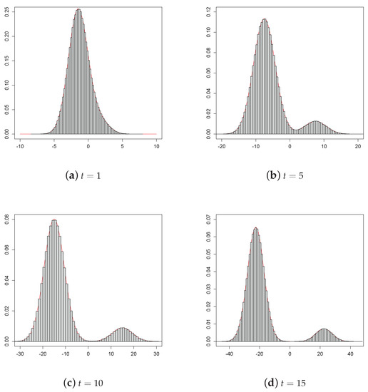
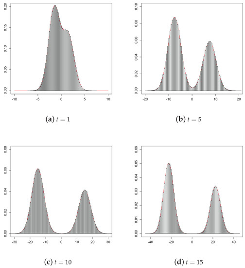
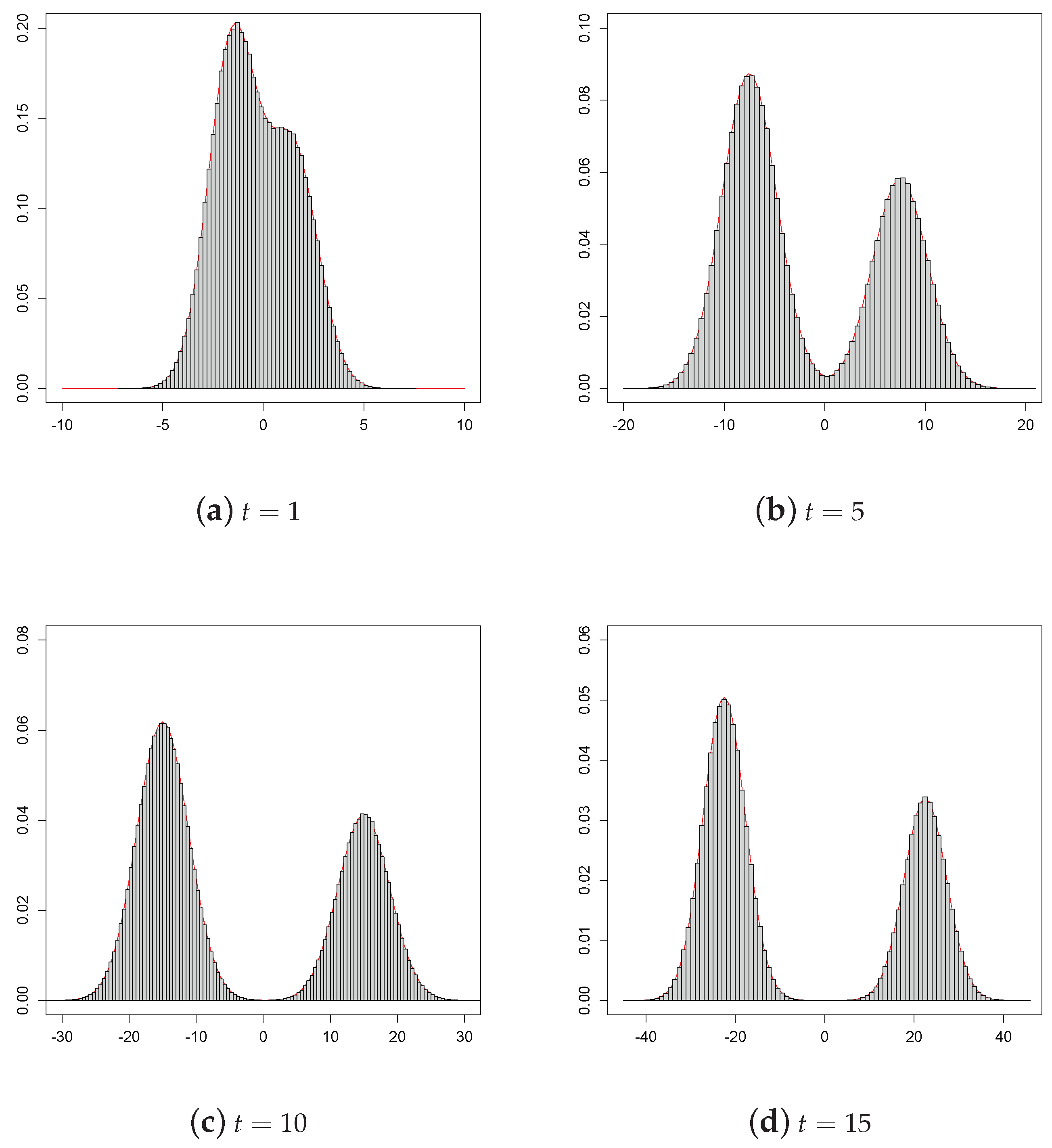
and $Z\left(t\right)\stackrel{d}{=}Y\left(t\right)$ for all fixed $t\ge 0$. Algorithm 1 can be used to compare the transition pdf (33) of $Z\left(t\right)$, being $\beta \left(t\right)$ and ${\sigma }^2\left(t\right)$ given in (41), with the histograms of the random sample of observations of $Y\left(t\right)$, obtained via (45), for different instants t. Specifically, in Figure 1, the histogram of a random sample of $N={10}^6$ observations of $Y\left(t\right)$ is obtained for different times t, by choosing $\beta \left(t\right)$ and ${\sigma }^2\left(t\right)$ as in (41), with $\vartheta =0.1$, $\gamma =1.5$, ${\sigma }^2=2$, $\nu =0.1$, $Q=1$.

Figure 1. For the process $Z\left(t\right)$, having infinitesimal moments (32), with $\vartheta =0.1$, $\beta \left(t\right)=1.5+0.2\pi sin\left(4\pi t\right)$ and ${\sigma }^2\left(t\right)=2$, the transition pdf (33) as a function of x is superimposed over a histogram obtained via Algorithm 1 for different choices of t.

In the sequel, we denote by

$$\mathrm{C}\left[Z\left(t\right)\right|Z\left(\tau \right)=y]=\frac{\sqrt{\mathrm{Var}\left[Z\right(t\left)\right|Z\left(\tau \right)=y]}}{\left|E\right[Z\left(t\right)\left|Z\right(\tau )=y]|}$$

the coefficient of variation. Making use of (34), in columns 2, 4, 6 of Table 1, the mean $E\left[Z\right(t\left)\right|Z\left(0\right)=0]$, the variance $\mathrm{Var}\left[Z\right(t\left)\right|Z\left(0\right)=0]$ and the coefficient of variation $\mathrm{C}\left[Z\right(t\left)\right|Z\left(0\right)=0]$ are listed for the same values of the parameters of Figure 1 with $t=1,5,10,15$. The values in columns 3, 5, 7 refer to the simulation sample mean ${\overline{y}}_t$, variance $s_t^2$ and coefficient of variation $c_t$, computed from the same random sample of $N={10}^6$ observations of $Y\left(t\right)$ used in Figure 1. The results of Figure 1 and Table 1 show the good agreement between the probabilistic results and those obtained via simulation.

Table 1. The conditional mean, variance, and coefficient of variation of $Z\left(t\right)$ are compared with the estimated values ${\overline{y}}_t$, $s_t^2$ and $c_t$ obtained by means of Algorithm 1 with the same choices of the parameters of Figure 1.

t	$\mathit{E}\left[\mathit{Z}\right(\mathit{t}\left)\right|\mathit{Z}\left(0\right)=0]$	${\overline{\mathit{y}}}_{\mathit{t}}$	$\mathbf{Var}\left[\mathit{Z}\right(\mathit{t}\left)\right|\mathit{Z}\left(0\right)=0]$	${\mathit{s}}_{\mathit{t}}^2$	$\mathbf{C}\left[\mathit{Z}\right(\mathit{t}\left)\right|\mathit{Z}\left(0\right)=0]$	${\mathit{c}}_{\mathit{t}}$
1	−1.200000	−1.201083	2.810000	2.81271	1.396921	1.396334
5	−6.0000000	−6.0033797	30.2500000	30.2705863	0.9166667	0.9164623
10	−12.0000000	−12.0057944	101.0000000	101.0350351	0.8374896	0.8372306
15	−18.0000000	−18.0080505	212.2500000	212.2809493	0.8093779	0.8090751

Algorithm 2 permits generating sample paths of the process $Y\left(t\right)$. Indeed, for the considered case, from (12), setting $t_1=0$, $Y\left(t_1\right)=0$, we have

$$Y\left(t_k\right)=Y\left(t_{k-1}\right)+R(t_{k-1},t_k)+\sigma \sqrt{t_k-t_{k-1}}{\xi }_k,k=2,3,\dots ,n,$$

(46)

where ${\xi }_1,{\xi }_2,\dots ,{\xi }_n$$\stackrel{iid}{=}$$\mathcal{N}(0,1)$ and

$$R(t_{k-1},t_k)=\left\{\begin{array}{cc}m\left(t_k\right)-m\left(t_{k-1}\right),\hfill & 0\le U_{k-1}<\vartheta ,0\le V_k<\vartheta ,\hfill \\ \\ m\left(t_k\right)+m\left(t_{k-1}\right),\hfill & \vartheta \le U_{k-1}<1,0\le V_k<\vartheta ,\hfill \\ \\ -m\left(t_k\right)-m\left(t_{k-1}\right),\hfill & 0\le U_{k-1}<\vartheta ,\vartheta \le V_k<1,\hfill \\ \\ -m\left(t_k\right)+m\left(t_{k-1}\right),\hfill & \vartheta \le U_{k-1}<1,\vartheta \le V_k<1,\hfill \end{array}\right.$$

(47)

with $m\left(t\right)$ given in (42).

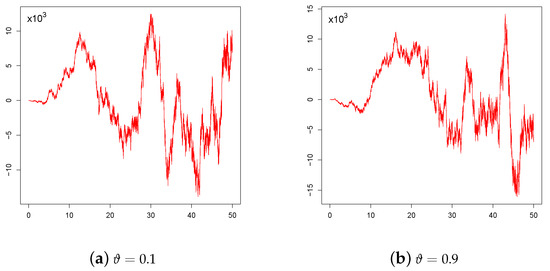
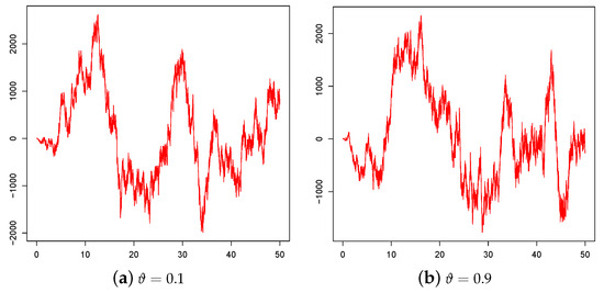
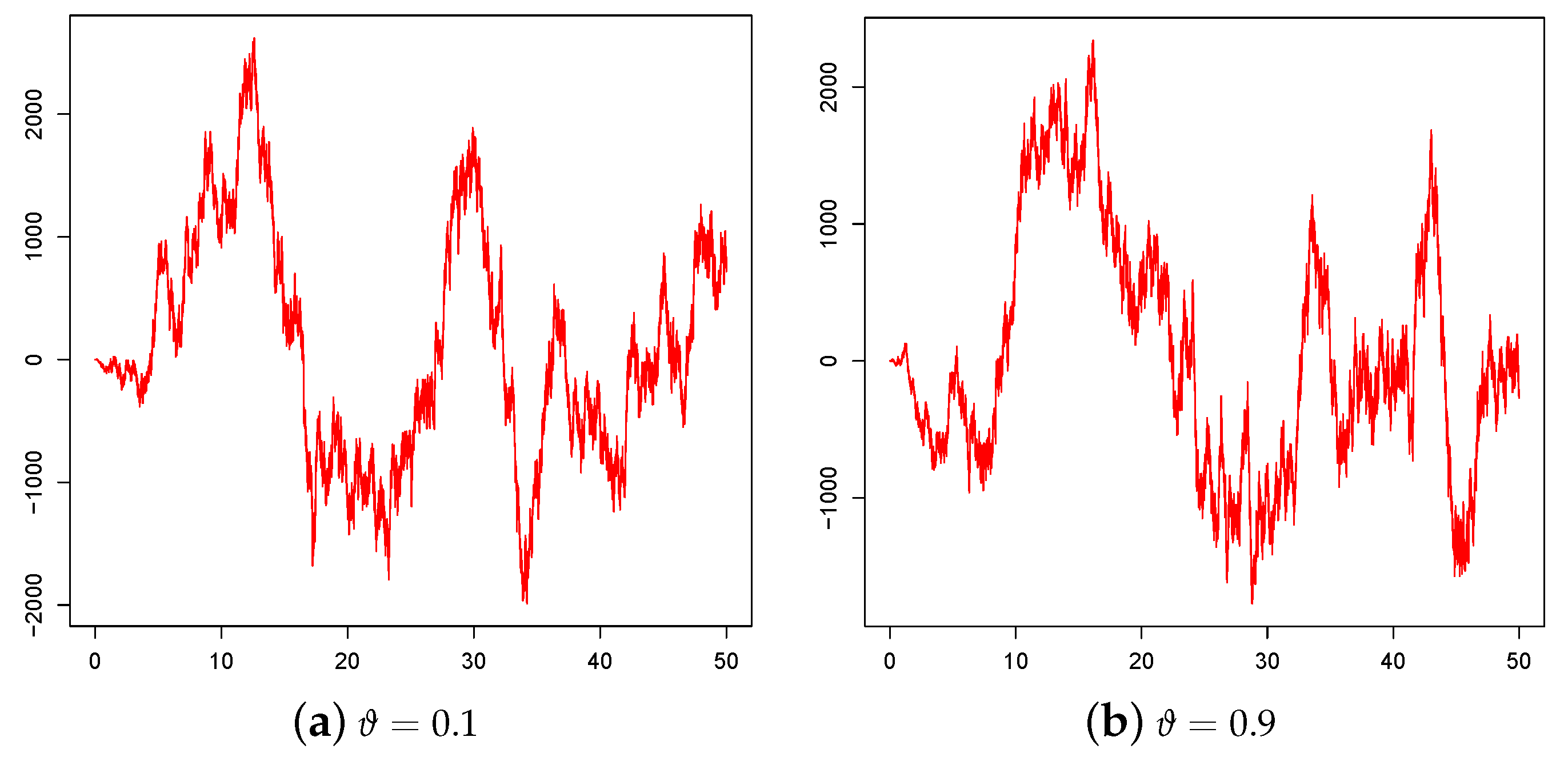
In Figure 2, a sample path of $Y\left(t\right)$ is plotted as function of t for $\vartheta =0.1$ and $\vartheta =0.9$ by choosing $\beta \left(t\right)$ and ${\sigma }^2\left(t\right)$ as in (41), with $\gamma =1.5$, ${\sigma }^2=2$, $\nu =0.1$, $Q=1$.

Figure 2. Simulated sample paths of the process $Y\left(t\right)$, obtained via (46) with $R(t_{k-1},t_k)$ given in (47), with $\beta \left(t\right)=1.5+0.2\pi sin\left(4\pi t\right)$ and ${\sigma }^2\left(t\right)=2$.

When $\vartheta =0$ or $\vartheta =1$, $Y\left(t\right)$ identifies with a time-inhomogeneous Wiener process $Z\left(t\right)$. Specifically, for $\vartheta =0$, $Z\left(t\right)$ has infinitesimal moments $B_1\left(t\right)=-\gamma -\frac{2\pi \nu }{Q}sin\left(\frac{4\pi t}{Q}\right)$ and $B_2={\sigma }^2$, whereas, when $\vartheta =1$, one has $B_1\left(t\right)=\gamma +\frac{2\pi \nu }{Q}sin\left(\frac{4\pi t}{Q}\right)$ and $B_2={\sigma }^2$. We recall that, for the time-homogeneous Wiener process $\tilde{Z}\left(t\right)$ with infinitesimal moments ${\tilde{B}}_1=\mu$ and ${\tilde{B}}_2={\sigma }^2$, the FTP pdf through the constant boundary S is known in closed form:

$$g(S,t|y,0)=\frac{|S-y|}{\sigma \sqrt{2\pi t^3}}exp\left\{-\frac{{(S-y-\mu t)}^2}{2{\sigma }^{2}t}\right\},y\ne S.$$

(48)

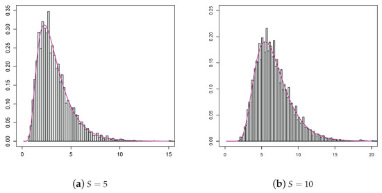
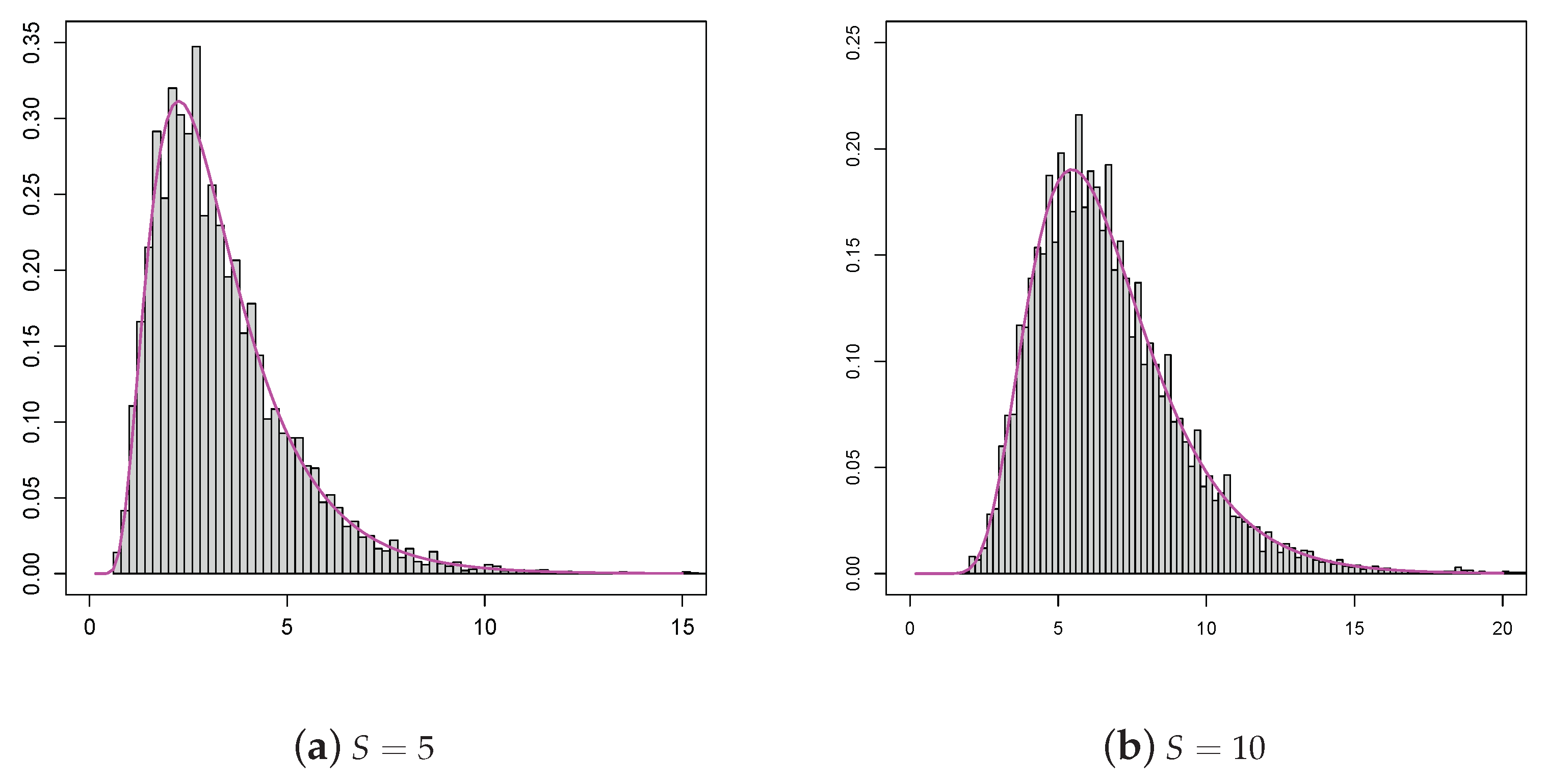
In Figure 3, for $\vartheta =1$, the histograms of FPT for $Z\left(t\right)$, with $\gamma =1.5,\nu =0.1,Q=1,{\sigma }^2=2$, from $Z\left(0\right)=0$ through a constant boundaries $S=5,10$ are plotted as function of t by using a collection of $N={10}^4$ simulated first passage times obtained via Algorithm 3. The solid curves in Figure 3 show the FPT densities of the Wiener process $\tilde{Z}\left(t\right)$, having infinitesimal moments ${\tilde{B}}_1=1.5$ and ${\tilde{B}}_2=2$, from $\tilde{Z}\left(0\right)=0$ through $S=5,10$, given in (48).

Figure 3. Histograms of FPT through the boundary S for the process $Z\left(t\right)$, given in (43), with $\vartheta =1$, $\gamma =1.5,\nu =0.1,{\sigma }^2=2,Q=1$, are compared with the FPT densities (solid curve) of the Wiener process $\tilde{Z}\left(t\right)$ with drift $\mu =1.5$ and infinitesimal variance ${\sigma }^2=2$ from $\tilde{Z}\left(0\right)=0$ through S.

Example 2.

We consider the diffusion process $Z\left(t\right)$ in (32) with

$${\sigma }^2\left(t\right)=\beta \left(t\right)=\gamma +\frac{2\pi \nu }{Q}sin\left(\frac{4\pi t}{Q}\right),t\ge 0,$$

(49)

where $\gamma >2\pi \left|\nu \right|/Q$, to ensure that $B_2\left(t\right)>0$ for $t\ge 0$, so that, from (31), one has:

$$m\left(t\right)=h_1\left(t\right)=\gamma t+\nu {sin}^2\left(\frac{2\pi t}{Q}\right),h_2\left(t\right)=1,t\ge 0.$$

(50)

Then, from (36), for $t\ge 0$ and $x\in \mathbb{R}$, one has:

$$B_1(x,t)=\left[\gamma +\frac{2\pi \nu }{Q}sin\left(\frac{4\pi t}{Q}\right)\right]\frac{\vartheta -(1-\vartheta )e^{-2x}}{\vartheta +(1-\vartheta )e^{-2x}},B_2\left(t\right)=\gamma +\frac{2\pi \nu }{Q}sin\left(\frac{4\pi t}{Q}\right),$$

(51)

with $0\le \vartheta \le 1$. The assumption (b) is satisfies with $c=1$. In this case, from (7), we obtain:

$$\begin{array}{ccc}& & X_i\left(t\right)=y+{(-1)}^{3-i}\{\gamma (t-\tau )+\nu [{sin}^2\left(\frac{2\pi t}{Q}\right)-{sin}^2\left(\frac{2\pi \tau }{Q}\right)\left]\right\}\hfill \\ & & +\sqrt{\gamma (t-\tau )+\nu [{sin}^2\left(\frac{2\pi t}{Q}\right)-{sin}^2(\frac{2\pi \tau }{Q}\left)\right]}{\xi }_{\tau ,t},i=1,2;t\ge \tau ,\hfill \end{array}$$

(52)

with ${\xi }_{\tau ,t}\sim \mathcal{N}(0,1)$; hence, (4) holds with

$$Q_y\left(\vartheta \right)=\frac{\vartheta }{\vartheta +(1-\vartheta )e^{-2y}},0\le \vartheta \le 1.$$

(53)

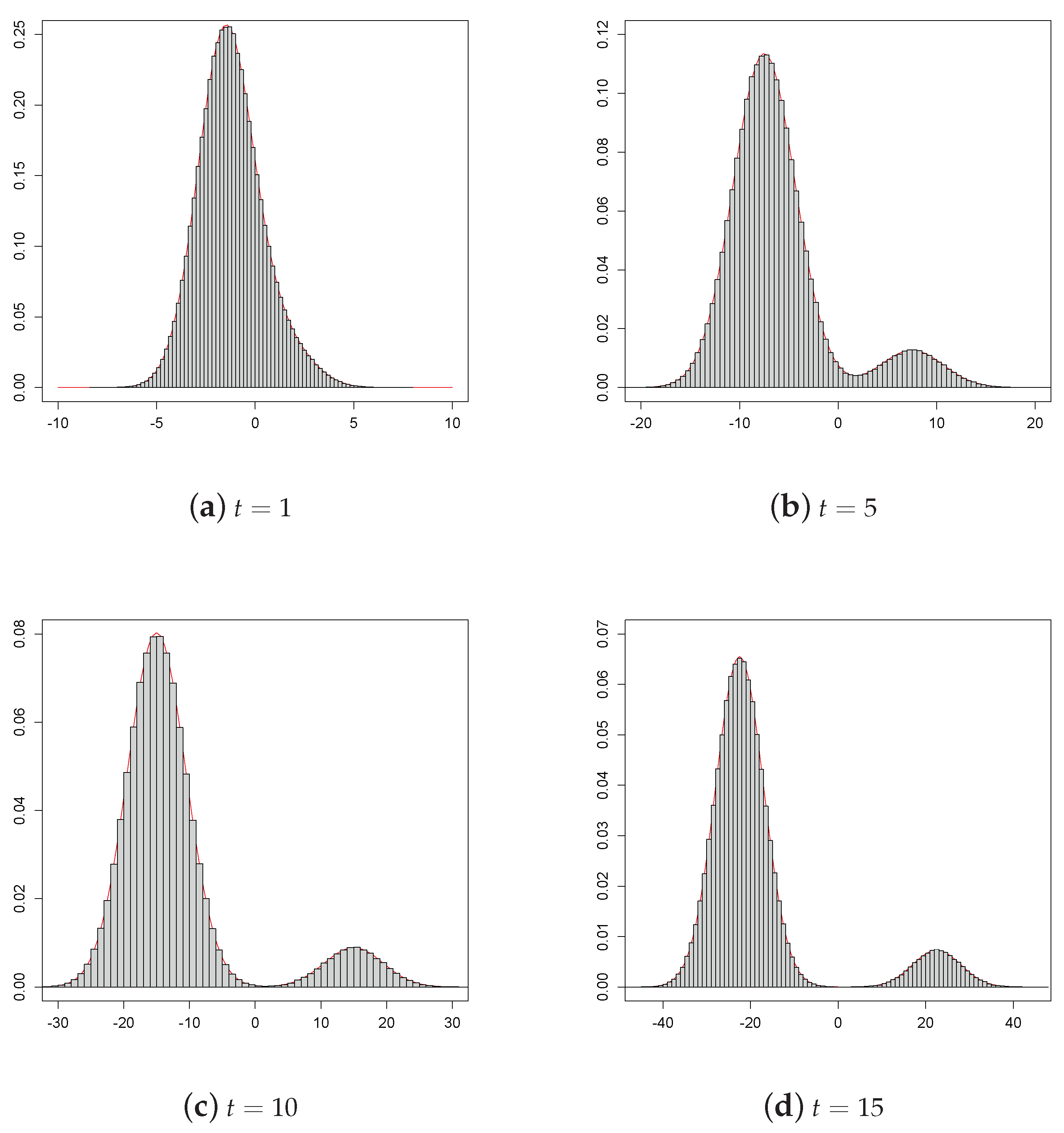
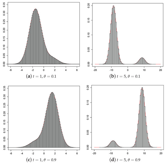
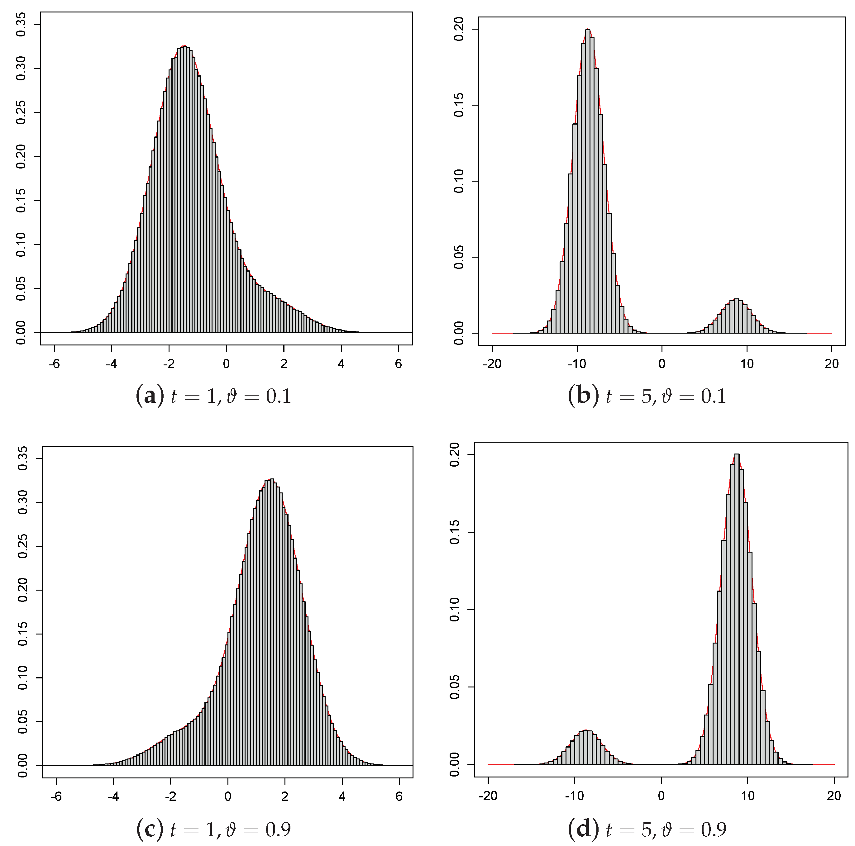
Since $Z\left(t\right)\stackrel{d}{=}Y\left(t\right)$ for all fixed $t\ge 0$, we use the Algorithm 1 to compare the transition pdf (37) of $Z\left(t\right)$ with the histograms of the random sample of observations of $Y\left(t\right)$ for different instants t. Specifically, in Figure 4, the histogram of a random sample of $N={10}^6$ observations of $Y\left(t\right)$ is obtained for different times t, by choosing $(y,\tau )=(0,0)$, $\beta \left(t\right)$ and ${\sigma }^2\left(t\right)$ as in (49), with $\vartheta =0.4$, $\gamma =1.5$, $\nu =0.1$, $Q=2$.

Figure 4. For the process $Z\left(t\right)$, having infinitesimal moments (51), with $(y,\tau )=(0,0)$ and $\vartheta =0.4$, $\gamma =1.5$, $\nu =0.1$, $Q=2$, the transition pdf (37) as a function of x is superimposed over a histogram obtained via Algorithm 1 for different choices of t.

For the same values of the parameters, in Table 2 for $t=1,5,10,15$, the conditional mean, variance, and coefficient of variation of $Z\left(t\right)$, evaluated via (38), are compared with the simulation sample mean ${\overline{y}}_t$, variance $s_t^2$ and coefficient of variation $c_t$, obtained making use of the same random sample of $N={10}^6$ observations of $Y\left(t\right)$ of Figure 4.

Table 2. For the same choices of the parameters of Figure 4, the conditional mean, variance, and coefficient of variation of $Z\left(t\right)$ are compared with the estimated values ${\overline{y}}_t$, $s_t^2$ and $c_t$, obtained by means of Algorithm 1.

t	$\mathit{E}\left[\mathit{Z}\right(\mathit{t}\left)\right|\mathit{Z}\left(0\right)=0]$	${\overline{\mathit{y}}}_{\mathit{t}}$	$\mathbf{Var}\left[\mathit{Z}\right(\mathit{t}\left)\right|\mathit{Z}\left(0\right)=0]$	${\mathit{s}}_{\mathit{t}}^2$	$\mathbf{C}\left[\mathit{Z}\right(\mathit{t}\left)\right|\mathit{Z}\left(0\right)=0]$	${\mathit{c}}_{\mathit{t}}$
1	−0.300000	−0.2997934	3.660000	3.6660900	6.377042	6.3867430
5	−1.500000	−1.497204	61.500000	61.576435	5.228129	5.241146
10	−3.000000	−2.993572	231.000000	231.231917	5.066228	5.079654
15	−4.500000	−4.489803	508.500000	508.947685	5.011099	5.024690

Furthermore, due to (39) and (40), for the diffusion process $Z\left(t\right)$ having infinitesimal moments (51), the FPT pdf through the boundary

$$S\left(t\right)=a_2+a_1\left[\gamma t+\nu {sin}^2\left(\frac{2\pi t}{Q}\right)\right],a_1,a_2\in \mathbb{R},\gamma >\frac{2\pi \left|\nu \right|}{Q},$$

(54)

is

$$\begin{array}{ccc}& & g_Z[S\left(t\right),t|y,\tau ]=\frac{|S\left(\tau \right)-y|\left[\gamma +\frac{2\pi \nu }{Q}sin\left(\frac{4\pi t}{Q}\right)\right]}{\gamma (t-\tau )+\nu [{sin}^2\left(\frac{2\pi t}{Q}\right)-{sin}^2(\frac{2\pi \tau }{Q}\left)\right]}{f}_Z[S\left(t\right),t|y,\tau ],\hfill \\ & & [y<S(\tau \left)\right]\mathrm{or}[y>S(\tau \left)\right].\hfill \end{array}$$

(55)

The first passage of $Z\left(t\right)$ through (54) is a certain event if and only if $[y<S\left(\tau \right),a_1\le -1]\mathrm{or}[y>S\left(\tau \right),a_1\ge 1]$.

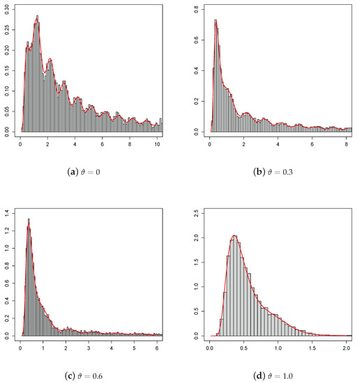
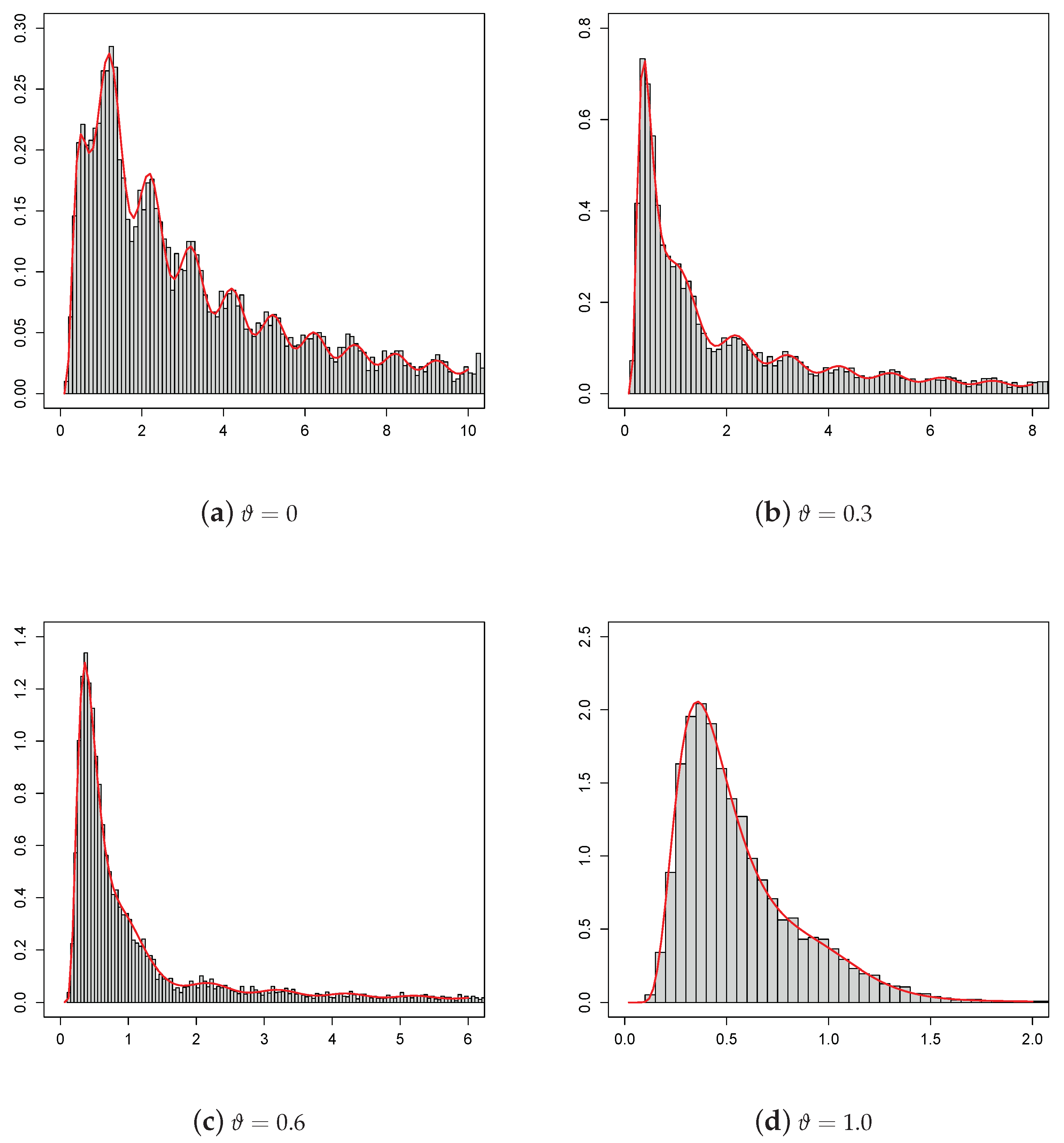
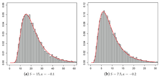
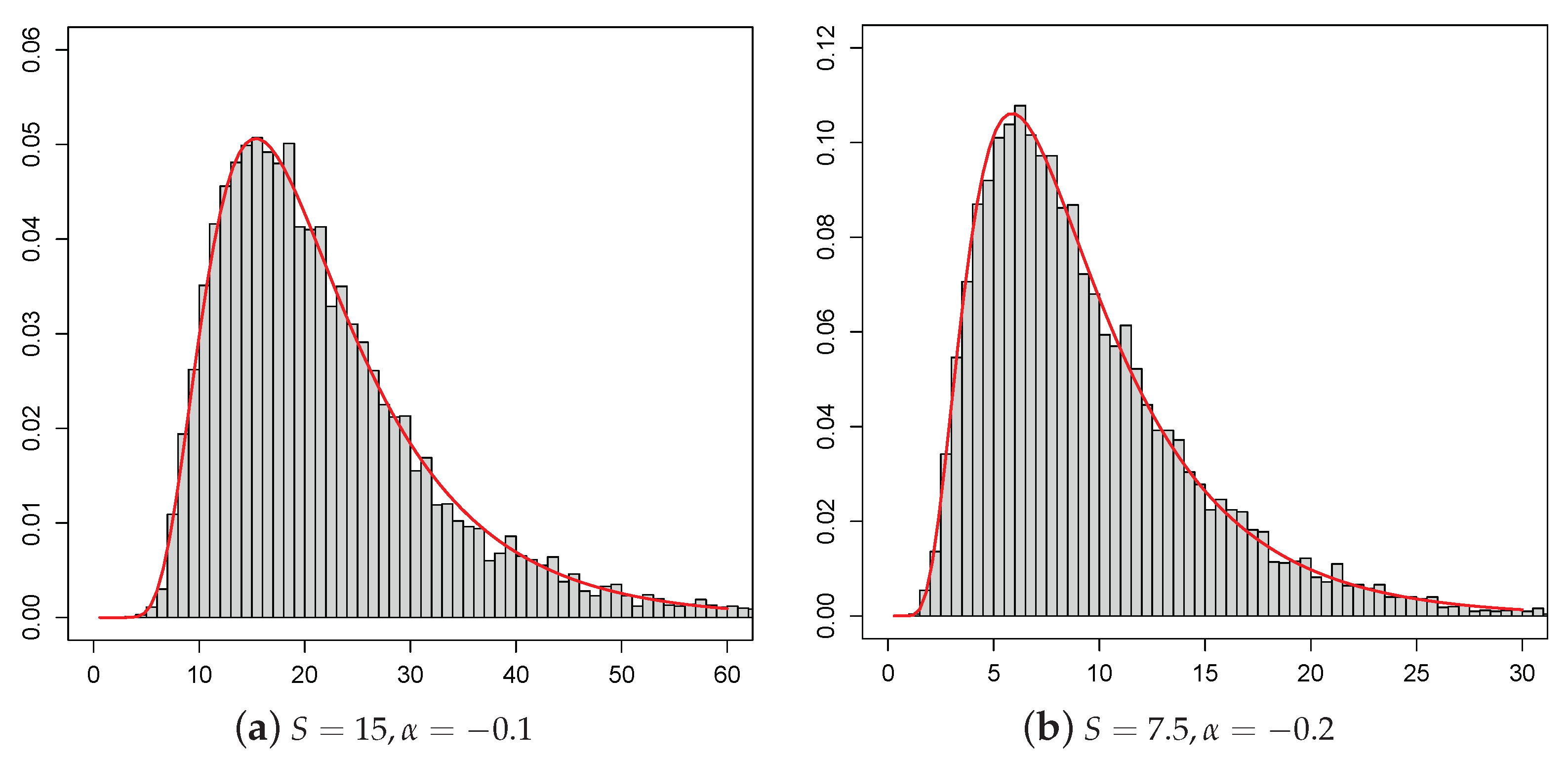
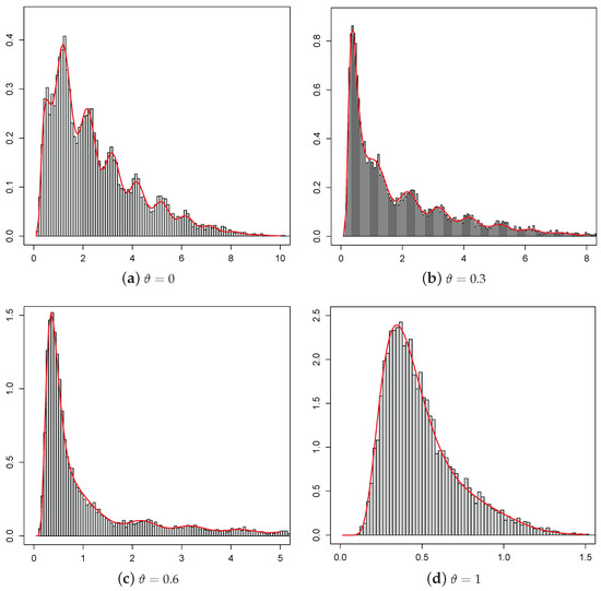
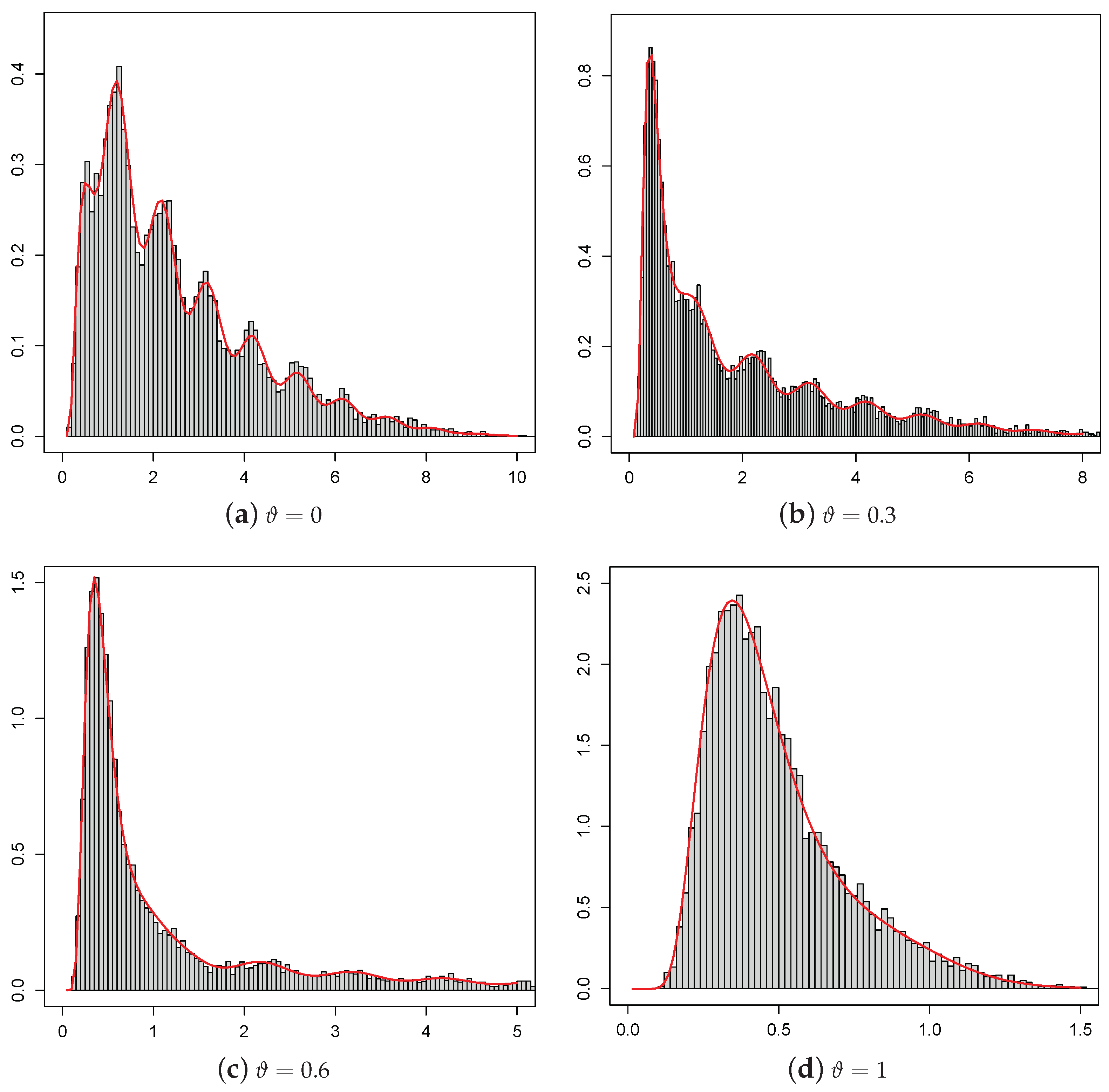
From (51), for $\vartheta =0$, one has $B_1\left(t\right)=-B_2\left(t\right)=-\gamma -\frac{2\pi \nu }{Q}sin\left(\frac{4\pi t}{Q}\right)$, whereas, when $\vartheta =1$, one obtains $B_1\left(t\right)=B_2\left(t\right)=\gamma +\frac{2\pi \nu }{Q}sin\left(\frac{4\pi t}{Q}\right)$; in both cases, $Y\left(t\right)=Z\left(t\right)$. In Figure 5, for some choices of ϑ, the histograms of FPT for the process (51), with $\gamma =1.5,\nu =0.1,Q=2$, from $Z\left(0\right)=0$ through (54), with $a_1=-1.2$, $a_2=2$ are plotted as a function of t by using a collection of $N={10}^4$ simulated first passage times obtained via Algorithm 3. The solid curves in Figure 5 show the FPT densities (55) with the same values of parameters.

Figure 5. Histograms of FPT through the boundary $S\left(t\right)=2-1.8t-0.12{sin}^2\left(\pi t\right)$ for the process $Z\left(t\right)$, given in (51), are compared with the FPT densities (solid curve), given in (55), for $y=0,\tau =0$ and $\gamma =1.5,\nu =0.1,Q=2$.

5. Simulation of Processes Generated via the Ornstein–Uhlenbeck Process

Let $X_1\left(t\right)$ and $X_2\left(t\right)$ be the time-inhomogeneous Ornstein–Uhlenbeck processes, with state-space in $\mathbb{R}$, conditioned to start from y at time $\tau$:

$$X_i\left(t\right)=y{e}^{\phi \left(t\right)-\phi \left(\tau \right)}+{(-1)}^{3-i}{e}^{\phi \left(t\right)}[\Lambda \left(t\right)-\Lambda \left(\tau \right)]+e^{\phi \left(t\right)}W\left[\Omega \left(t\right)-\Omega \left(\tau \right)\right],t\ge \tau ,$$

(56)

for $i=1,2$, where

$$\phi \left(t\right)={\int }_0^t\alpha \left(z\right)dz,\Lambda \left(t\right)={\int }_0^t\beta \left(u\right)e^{-\phi \left(u\right)}du,\Omega \left(t\right)={\int }_0^t{\sigma }^2\left(u\right)e^{-2\phi \left(u\right)}du,$$

(57)

being $\alpha \left(t\right)$, $\beta \left(t\right)$ and $\sigma \left(t\right)$ continuous functions, with $\alpha \left(t\right)\in \mathbb{R}$, $\beta \left(t\right)\in \mathbb{R}$ and $\sigma \left(t\right)>0$. By virtue of (1), for $t\ge 0$, one has:

$$m\left(t\right)=e^{\phi \left(t\right)}\Lambda \left(t\right),h_1\left(t\right)=e^{\phi \left(t\right)}\Omega \left(t\right),h_2\left(t\right)=e^{\phi \left(t\right)}.$$

(58)

From (14) and (58), we consider the diffusion process $Z\left(t\right)$ with infinitesimal moments:

$$B_1(x,t)=\alpha \left(t\right)x+\beta \left(t\right)\frac{{\displaystyle \vartheta -(1-\vartheta )exp\left\{-2x\frac{e^{-\phi \left(t\right)}\Lambda \left(t\right)}{\Omega \left(t\right)}\right\}}}{{\displaystyle \vartheta +(1-\vartheta )exp\left\{-2x\frac{e^{-\phi \left(t\right)}\Lambda \left(t\right)}{\Omega \left(t\right)}\right\}}},B_2\left(t\right)={\sigma }^2\left(t\right),$$

(59)

with $0\le \vartheta \le 1$. If $\alpha \left(t\right)=0$ for all $t\ge 0$, then the drift in (59) is identified with that in (32). Furthermore, if $\vartheta =0$, $Z\left(t\right)=X_2\left(t\right)$ is the time-inhomogeneous Ornstein–Uhlenbeck process with infinitesimal moments $B_1(x,t)=\alpha \left(t\right)x-\beta \left(t\right)$ and $B_2\left(t\right)={\sigma }^2\left(t\right)$, whereas, when $\vartheta =1$, $Z\left(t\right)=X_1\left(t\right)$ is the time-inhomogeneous Ornstein–Uhlenbeck process with infinitesimal moments $B_1(x,t)=\alpha \left(t\right)x+\beta \left(t\right)$ and $B_2\left(t\right)={\sigma }^2\left(t\right)$.

We assume that $\beta \left(t\right)\ne 0$ for all $t\ge 0$. By choosing $(y,\tau )=(0,0)$, from (58), one has $m\left(0\right)=h_1\left(0\right)=0$; hence, the assumptions (a) are satisfied, and, from (15), one has:

$$\begin{array}{ccc}& & {\displaystyle f_Z(x,t|0,0)=e^{-\phi \left(t\right)}\left[\vartheta +(1-\vartheta )exp\left\{-2x\frac{e^{-\phi \left(t\right)}\Lambda \left(t\right)}{\Omega \left(t\right)}\right\}\right]}\hfill \\ & & \times \frac{1}{\sqrt{2\pi \Omega \left(t\right)}}exp\left\{-\frac{{\left[x{e}^{-\phi \left(t\right)}-\Lambda \left(t\right)\right]}^2}{2\Omega \left(t\right)}\right\},x\in \mathbb{R},\hfill \end{array}$$

(60)

and, making use of (58) in (16), one obtains:

$$\begin{array}{cc}\hfill E\left[Z\right(t\left)\right|Z\left(0\right)=0|& =(2\vartheta -1)e^{\phi \left(t\right)}\Lambda \left(t\right),\hfill \\ \hfill \mathrm{Var}\left[Z\right(t\left)\right|Z\left(0\right)=0]& =e^{2\phi \left(t\right)}\Omega \left(t\right)+4\vartheta (1-\vartheta )e^{2\phi \left(t\right)}{\Lambda }^2\left(t\right),\hfill \end{array}$$

(61)

where $\phi \left(t\right)$, $\Lambda \left(t\right)$ and $\Omega \left(t\right)$ are given in (57). Moreover, the assumption (b) holds if and only if

$$\beta \left(t\right)=c{e}^{-\phi \left(t\right)}{\sigma }^2\left(t\right),t\ge 0,c\in \mathbb{R}.$$

(62)

In this case, from (59), the infinitesimal moments of $Z\left(t\right)$ are:

$$B_1(x,t)=\alpha \left(t\right)x+\beta \left(t\right)\frac{\vartheta -(1-\vartheta )exp\{-2cx{e}^{-\phi \left(t\right)}\}}{\vartheta +(1-\vartheta )exp\{-2cx{e}^{-\phi \left(t\right)}\}},B_2\left(t\right)={\sigma }^2\left(t\right),$$

(63)

with $0\le \vartheta \le 1$, and, from (18), one has

$$\begin{array}{ccc}& & f_Z(x,t|y,\tau )=\frac{\vartheta +(1-\vartheta )exp\{-2cx{e}^{-\phi \left(t\right)}\}}{\vartheta +(1-\vartheta )exp\{-2cy{e}^{-\phi \left(\tau \right)}\}}\frac{e^{-\phi \left(t\right)}}{\sqrt{2\pi [\Omega (t)-\Omega (\tau \left)\right]}}\hfill \\ & & {\displaystyle \times exp\left\{-\frac{{\left[x{e}^{-\phi \left(t\right)}-y{e}^{-\phi \left(\tau \right)}-c[\Omega \left(t\right)-\Omega \left(\tau \right)]\right]}^2}{2[\Omega (t)-\Omega (\tau \left)\right]}\right\},x,y\in \mathbb{R}.}\hfill \end{array}$$

(64)

Making use of (58) in (19), one obtains:

$$\begin{array}{ccc}& & E[Z\left(t\right)|Z\left(\tau \right)=y|=y{e}^{\phi \left(t\right)-\phi \left(\tau \right)}+c{e}^{\phi \left(t\right)}[\Omega \left(t\right)-\Omega \left(\tau \right)]\frac{\vartheta -(1-\vartheta )exp\left\{-2cy{e}^{-\phi \left(\tau \right)}\right\}}{\vartheta +(1-\vartheta )exp\left\{-2cy{e}^{-\phi \left(\tau \right)}\right\}},\hfill \\ & & \mathrm{Var}\left[Z\left(t\right)\right|Z\left(\tau \right)=y]=e^{2\phi \left(t\right)}[\Omega \left(t\right)-\Omega \left(\tau \right)]+c^2{e}^{2\phi \left(t\right)}{[\Omega \left(t\right)-\Omega \left(\tau \right)]}^2\hfill \\ & & \times \frac{4\vartheta (1-\vartheta )exp\left\{-2cy{e}^{-\phi \left(\tau \right)}\right\}}{{\left[\vartheta +(1-\vartheta )exp\left\{-2cy{e}^{-\phi \left(\tau \right)}\right\}\right]}^2},\hfill \end{array}$$

(65)

with $\phi \left(t\right)$, $\Lambda \left(t\right)$ and $\Omega \left(t\right)$ defined in (57). Furthermore, due to (27) and (28), the FPT pdf of the process $Z\left(t\right)$ through the boundary

$$S\left(t\right)=e^{\phi \left(t\right)}\left[a_2+a_1\Omega \left(t\right)\right],t\ge 0,a_1,a_2\in \mathbb{R}$$

(66)

is

$$g_Z[S\left(t\right),t|y,\tau ]=\frac{|S\left(\tau \right)-y|e^{-\phi \left(t\right)-\phi \left(\tau \right)}}{\Omega \left(t\right)-\Omega \left(\tau \right)}{\sigma }^2\left(t\right)f_Z[S\left(t\right),t|y,\tau ],[y<S\left(\tau \right)]\mathrm{or}[y>S\left(\tau \right)],$$

(67)

with $f_Z(x,t|y,\tau )$ given in (64). Finally, the first passage of $Z\left(t\right)$ through $S\left(t\right)$, given in (66), is a certain event if and only if $[S\left(\tau \right)-y][a_1+{(-1)}^{i}c]\le 0$ for $i=1,2$.

Example 3.

We consider the diffusion process $Z\left(t\right)$ in (59) with

$$\alpha \left(t\right)=\alpha ,\beta \left(t\right)=\beta ,{\sigma }^2\left(t\right)={\sigma }^2,t\ge 0.$$

(68)

Therefore, from (57), one has

$$\phi \left(t\right)=\alpha t,\Lambda \left(t\right)=\frac{\beta }{\alpha }(1-e^{-\alpha t}),\Omega \left(t\right)=\frac{{\sigma }^2}{2\alpha }(1-e^{-2\alpha t}),t\ge 0,$$

(69)

so that

$$m\left(t\right)=\frac{\beta }{\alpha }(e^{\alpha t}-1),h_1\left(t\right)=\frac{{\sigma }^2}{2\alpha }(e^{\alpha t}-e^{-\alpha t}),h_2\left(t\right)=e^{\alpha t},t\ge 0.$$

(70)

Then, from (59), it follows that the infinitesimal moments of $Z\left(t\right)$ are

$$B_1(x,t)=\alpha x+\beta \frac{{\displaystyle \vartheta -(1-\vartheta )exp\left\{-\frac{4\beta x}{{\sigma }^2(1+e^{\alpha t})}\right\}}}{{\displaystyle \vartheta +(1-\vartheta )exp\left\{-\frac{4\beta x}{{\sigma }^2(1+e^{\alpha t})}\right\}}},B_2\left(t\right)={\sigma }^2,$$

(71)

with $0\le \vartheta \le 1$. We suppose that $(y,\tau )=(0,0)$, so that the assumptions (a) are satisfied. From (60), one has:

$$\begin{array}{ccc}& & f_Z(x,t|0,0)=\left[\vartheta +(1-\vartheta )exp\left\{-\frac{4\beta x}{{\sigma }^2(1+e^{\alpha t})}\right\}\right]\sqrt{\frac{\alpha }{\pi {\sigma }^2(e^{2\alpha t}-1)}}\hfill \\ & & \times exp\left\{-\frac{\alpha {\left[x-\frac{\beta }{\alpha }(e^{\alpha t}-1)\right]}^2}{{\sigma }^2(e^{2\alpha t}-1)}\right\},x\in \mathbb{R}.\hfill \end{array}$$

(72)

We note that, for $\alpha <0$, the process $Z\left(t\right)$ admits a steady-state density:

$$\begin{array}{ccc}& & {\displaystyle W_Z\left(x\right)=\underset{t\to +\infty }{lim}{f}_Z(x,t|0,0)=\left[\vartheta +(1-\vartheta )exp\left\{-\frac{4\beta x}{{\sigma }^2}\right\}\right]}\hfill \\ & & \times \sqrt{\frac{\left|\alpha \right|}{\pi {\sigma }^2}}exp\left\{-\frac{\left|\alpha \right|}{{\sigma }^2}{\left(x-\frac{\beta }{\left|\alpha \right|}\right)}^2\right\},x\in \mathbb{R}.\hfill \end{array}$$

(73)

From (7), we have:

$$X_i\left(t\right)={(-1)}^{3-i}\beta \frac{e^{\alpha t}-1}{\alpha }+\sigma \sqrt{\frac{e^{2\alpha t}-1}{2\alpha }}{\xi }_t,i=1,2;t\ge 0,$$

(74)

with ${\xi }_t\sim \mathcal{N}(0,1)$. Recalling (4) and (5), $Y\left(t\right)$ is given in (45) with $X_i\left(t\right)$ given in (74) and $Z\left(t\right)\stackrel{d}{=}Y\left(t\right)$ for all fixed $t\ge 0$.

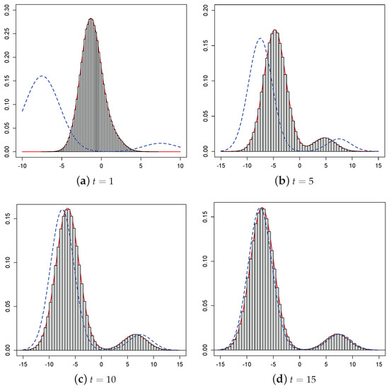
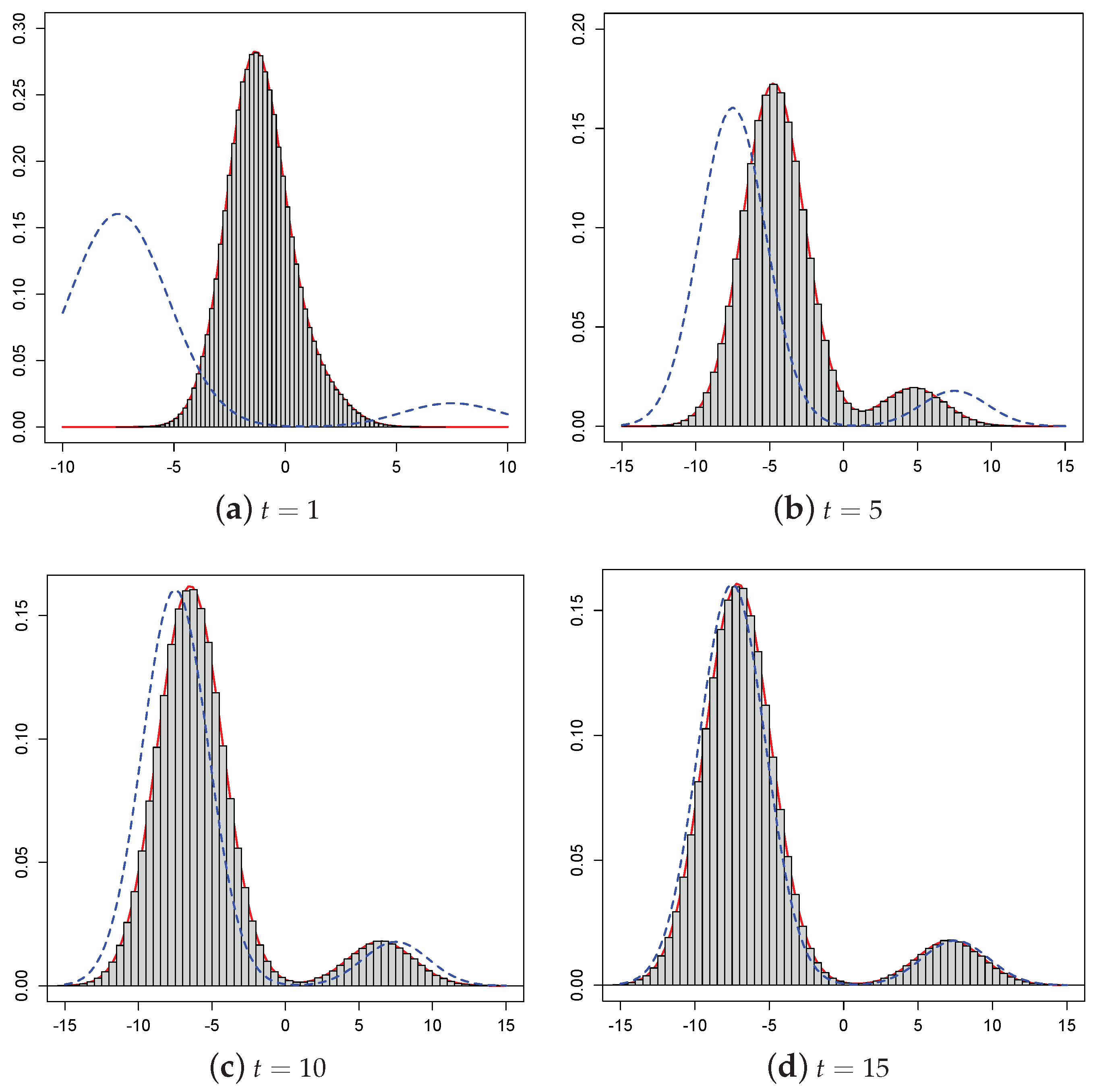
In Figure 5, we compare the transition densities (72) of $Z\left(t\right)$ with the histograms of the random sample of observations of $Y\left(t\right)$ for different instants t, obtained by using Algorithm 1. The histogram of a random sample of $N={10}^6$ observations of $Y\left(t\right)$ is obtained for different times t, by choosing $\vartheta =0.1$, $\alpha =-0.2$, $\beta =1.5$, ${\sigma }^2=2.0$. The dashed curves in Figure 5 show the steady-state density (73) for the same choices of parameters.

For the same values of the parameters, in Table 3 for $t=1,5,10,15$, the conditional mean, variance, and coefficient of variation of $Z\left(t\right)$, evaluated via (61), are compared with the simulation sample mean ${\overline{y}}_t$, variance $s_t^2$ and coefficient of variation $c_t$, obtained making use of the same random sample of $N={10}^6$ observations of $Y\left(t\right)$ of Figure 6.

Table 3. For the same choices of the parameters of Figure 6, the conditional mean, variance, and coefficient of variation of $Z\left(t\right)$ are compared with the estimated values ${\overline{y}}_t$, $s_t^2$ and $c_t$, obtained by means of Algorithm 1.

t	$\mathit{E}\left[\mathit{Z}\right(\mathit{t}\left)\right|\mathit{Z}\left(0\right)=0]$	${\overline{\mathit{y}}}_{\mathit{t}}$	$\mathbf{Var}\left[\mathit{Z}\right(\mathit{t}\left)\right|\mathit{Z}\left(0\right)=0]$	${\mathit{s}}_{\mathit{t}}^2$	$\mathbf{C}\left[\mathit{Z}\right(\mathit{t}\left)\right|\mathit{Z}\left(0\right)=0]$	${\mathit{c}}_{\mathit{t}}$
1	−1.087615	−1.088598	2.313785	2.316015	1.398576	1.397987
5	−3.7927234	−3.7949015	12.4147457	12.4236120	0.9290044	0.9288026
10	−5.1879883	−5.1906403	20.0482345	20.0579186	0.8630562	0.8628236
15	−5.7012776	−5.7040871	23.2714247	23.2806625	0.8461343	0.8458854

Figure 6. For the process $Z\left(t\right)$ having infinitesimal moments (71), with $\vartheta =0.1$, $\alpha =-0.2$, $\beta =1.5$, ${\sigma }^2=2$, the transition pdf (72) as a function of x is superimposed over a histogram obtained via Algorithm 1 for different choices of t. The dashed curves indicate the steady-state pdf given in (73).

Applying the Algorithm 2, we generate sample paths of the process $Y\left(t\right)$. For the considered case, from (12), by setting $t_1=0$, $Y\left(t_1\right)=0$, we have:

$$Y\left(t_k\right)=Y\left(t_{k-1}\right)e^{\alpha (t_k-t_{k-1})}+R(t_{k-1},t_k)+\sigma e^{\alpha t_k}\sqrt{\frac{e^{-2\alpha t_{k-1}}-e^{-2\alpha t_k}}{2\alpha }}{\xi }_k,$$

(75)

where ${\xi }_1,{\xi }_2,\dots ,{\xi }_n$$\stackrel{iid}{=}$$\mathcal{N}(0,1)$ and

$$R(t_{k-1},t_k)=\left\{\begin{array}{cc}m\left(t_k\right)-m\left(t_{k-1}\right)e^{\alpha (t_k-t_{k-1})},\hfill & 0\le U_{k-1}<\vartheta ,0\le V_k<\vartheta ,\hfill \\ \\ m\left(t_k\right)+m\left(t_{k-1}\right)e^{\alpha (t_k-t_{k-1})},\hfill & \vartheta \le U_{k-1}<1,0\le V_k<\vartheta ,\hfill \\ \\ -m\left(t_k\right)-m\left(t_{k-1}\right)e^{\alpha (t_k-t_{k-1})},\hfill & 0\le U_{k-1}<\vartheta ,\vartheta \le V_k<1,\hfill \\ \\ -m\left(t_k\right)+m\left(t_{k-1}\right)e^{\alpha (t_k-t_{k-1})},\hfill & \vartheta \le U_{k-1}<1,\vartheta \le V_k<1,\hfill \end{array}\right.$$

(76)

with $m\left(t\right)$ given in (70).

In Figure 7, a sample path of $Y\left(t\right)$ is plotted as function of t for $\vartheta =0.1$ and $\vartheta =0.9$ by using (75) with $\alpha =-0.2$, $\beta =1.5$ and ${\sigma }^2=2$.

Figure 7. Simulated sample paths of the process $Y\left(t\right)$ obtained via (75), where $R(t_{k-1},t_k)$ is given in (76) with $\alpha =-0.2$, $\beta =1.5$ and ${\sigma }^2=2$.

When $\vartheta =0$ or $\vartheta =1$, $Y\left(t\right)$ identifies with a time-homogeneous Ornstein–Uhlenbeck process $Z\left(t\right)$. In particular, for $\vartheta =0$, $Z\left(t\right)$ has infinitesimal moments $B_1\left(x\right)=\alpha x-\beta$ and $B_2={\sigma }^2$, whereas, when $\vartheta =1$, one has $B_1\left(x\right)=\alpha x+\beta$ and $B_2={\sigma }^2$. We recall that, for the time-homogeneous Ornstein–Uhlenbeck process $\tilde{Z}\left(t\right)$ with infinitesimal moments ${\tilde{B}}_1\left(x\right)=\alpha x+\beta$ and ${\tilde{B}}_2={\sigma }^2$, the FTP pdf through the constant boundary $S=-\beta /\alpha$ is known in closed form:

$$g\left(-\frac{\beta }{\alpha },t|y,0\right)=\frac{2e^{\alpha t}|y+\beta /\alpha |}{\sigma \sqrt{\pi }}{\left(\frac{\alpha }{e^{2\alpha t}-1}\right)}^{3/2}exp\left\{-\frac{\alpha e^{2\alpha t}{(y+\beta /\alpha )}^2}{{\sigma }^2(e^{2\alpha t}-1)}\right\},y\ne -\beta /\alpha .$$

(77)

In Figure 8, for $\vartheta =1$, the histograms of FPT for $Z\left(t\right)$, with $\beta =1.5$, ${\sigma }^2=2$, $\alpha =-0.1$ on the left and $\alpha =-0.2$ on the right, from $Z\left(0\right)=0$ through the constant boundary $S=15$ (on the left) and $S=7.5$ (on the right) are plotted as a function of t by using a collection of $N={10}^4$ simulated first passage times obtained via Algorithm 3. The solid curves in Figure 8 refer to the closed expression of FPT densities for the Ornstein–Uhlenbeck process from $Z\left(0\right)=0$ through $S=-\beta /\alpha$, given in (77).

Figure 8. Histograms of FPT through the boundary S for the process $Z\left(t\right)$, given in (43), with $\vartheta =1$, $\beta =1.5,{\sigma }^2=2$, are compared with the FPT densities (solid curve) of the Ornstein–Uhlenbeck process from $Z\left(0\right)=0$ through $S=-\beta /\alpha$.

Example 4.

Let $Z\left(t\right)$ be the diffusion process having infinitesimal drift and infinitesimal variance given in (59) with

$$\alpha \left(t\right)=\alpha ,{\sigma }^2\left(t\right)=\gamma +\frac{2\pi \nu }{Q}sin\left(\frac{4\pi t}{Q}\right),\beta \left(t\right)=e^{-\alpha t}{\sigma }^2\left(t\right),t\ge 0,$$

(78)

where $\gamma >2\pi \left|\nu \right|/Q$. Therefore, from (57), one has

$$\begin{array}{cc}& \phi \left(t\right)=\alpha t,\hfill \\ & \Lambda \left(t\right)=\Omega \left(t\right)=\gamma \frac{1-e^{-2\alpha t}}{2\alpha }-\frac{\nu \pi e^{-2\alpha t}}{4{\pi }^2+{\alpha }^2{Q}^2}\left[2\pi cos\left(\frac{4\pi t}{Q}\right)+\alpha Qsin\left(\frac{4\pi t}{Q}\right)-2\pi e^{2\alpha t}\right],\hfill \end{array}$$

(79)

so that, from (58), one has:

$$m\left(t\right)=h_1\left(t\right)=e^{\alpha t}\Omega \left(t\right),h_2\left(t\right)=e^{\alpha t},t\ge 0.$$

(80)

From (63), one has

$$\begin{array}{cc}\hfill & B_1(x,t)=\alpha x+e^{-\alpha t}\left[\gamma +\frac{2\pi \nu }{Q}sin\left(\frac{4\pi t}{Q}\right)\right]\frac{\vartheta -(1-\vartheta )exp\{-2x{e}^{-\alpha t}\}}{\vartheta +(1-\vartheta )exp\{-2x{e}^{-\alpha t}\}},\hfill \\ \hfill & B_2\left(t\right)=\gamma +\frac{2\pi \nu }{Q}sin\left(\frac{4\pi t}{Q}\right),\hfill \end{array}$$

(81)

with $\gamma >2\pi \left|\nu \right|/Q$. The assumption (b) is satisfied with $c=1$. In this case, from (7), we obtain:

$$X_i\left(t\right)=y{e}^{\alpha (t-\tau )}+{(-1)}^{3-i}{e}^{\alpha t}\left[\Omega \left(t\right)-\Omega \left(\tau \right)\right]+e^{\alpha t}\sqrt{\Omega \left(t\right)-\Omega \left(\tau \right)}{\xi }_{\tau ,t},t\ge \tau ,$$

(82)

where ${\xi }_{\tau ,t}\sim \mathcal{N}(0,1)$. Then, (4) holds with

$$Q_{y,\tau }\left(\vartheta \right)=\frac{\vartheta }{\vartheta +(1-\vartheta )exp\left\{-2e^{-\alpha \tau }y\right\}},0\le \vartheta \le 1.$$

(83)

Being $Z\left(t\right)\stackrel{d}{=}Y\left(t\right)$ for all fixed $t\ge 0$, Algorithm 1 can be used to compare the transition pdf (64) of $Z\left(t\right)$ with the histograms of the random sample of observations of $Y\left(t\right)$ for different instants t. Specifically, in Figure 9, the histogram of a random sample of $N={10}^6$ observations of $Y\left(t\right)$ is obtained for different times t, by choosing $\alpha \left(t\right)$, $\beta \left(t\right)$ and ${\sigma }^2\left(t\right)$ as in (78), with $(y,\tau )=(0,0)$ and $\vartheta =0.1$, $\alpha =-0.2$, $\gamma =1.5$, $\nu =0.1$, $Q=2$. Note that Figure 9c,d are mirrored to Figure 9a,b, respectively.

Figure 9. For the process $Z\left(t\right)$ having infinitesimal moments (81), with $(y,\tau )=(0,0)$ and $\alpha =-0.2$, $\gamma =1.5$, $\nu =0.1$, $Q=2$, the transition pdf (64) as a function of x is superimposed over a histogram obtained via Algorithm 1 for different choices of t.

For the same values of the parameters with $\vartheta =0.1$, in Table 4, for $t=1,5,10,15$ the conditional mean, variance, and coefficient of variation of $Z\left(t\right)$, evaluated via (65), are compared with the simulation sample mean ${\overline{y}}_t$, variance $s_t^2$ and coefficient of variation $c_t$, obtained making use of the same random sample of $N={10}^6$ observations of $Y\left(t\right)$ of Figure 9.

Table 4. For the same choices of the parameters of Figure 9 with $\vartheta =0.1$, the conditional mean, variance, and coefficient of variation of $Z\left(t\right)$ are compared with the estimated values ${\overline{y}}_t$, $s_t^2$ and $c_t$, obtained by means of Algorithm 1.

t	$\mathit{E}\left[\mathit{Z}\right(\mathit{t}\left)\right|\mathit{Z}\left(0\right)=0]$	${\overline{\mathit{y}}}_{\mathit{t}}$	$\mathbf{Var}\left[\mathit{Z}\right(\mathit{t}\left)\right|\mathit{Z}\left(0\right)=0]$	${\mathit{s}}_{\mathit{t}}^2$	$\mathbf{C}\left[\mathit{Z}\right(\mathit{t}\left)\right|\mathit{Z}\left(0\right)=0]$	${\mathit{c}}_{\mathit{t}}$
1	−1.191974	−1.192894	2.019084	2.021058	1.192094	1.191757
5	−6.9575706	−6.9605112	30.4288148	30.4284625	0.7928388	0.7924993
10	−21.4721848	−21.4793776	262.9543652	262.8009005	0.7552343	0.7547302
15	−59.3090545	−59.3271807	1982.3207516	1980.5425005	0.7506992	0.7501332

Furthermore, for the diffusion process $Z\left(t\right)$ having infinitesimal moments (81), the FPT pdf through the boundary

$$S\left(t\right)=e^{\alpha t}\left\{a_2+a_1\gamma \frac{1-e^{-2\alpha t}}{2\alpha }-\frac{a_1\nu \pi e^{-2\alpha t}}{4{\pi }^2+{\alpha }^2{Q}^2}\left[2\pi cos\left(\frac{4\pi t}{Q}\right)+\alpha Qsin\left(\frac{4\pi t}{Q}\right)-2\pi e^{2\alpha t}\right]\right\},$$

(84)

with $a_1,a_2\in \mathbb{R}$ and $\gamma >2\pi \left|\nu \right|/Q$, is

$$\begin{array}{cc}& g_Z[S\left(t\right),t|y,\tau ]=\frac{|S\left(\tau \right)-y|e^{-\alpha (t+\tau )}}{\Omega \left(t\right)-\Omega \left(\tau \right)}\left[\gamma +\frac{2\pi \nu }{Q}sin\left(\frac{4\pi t}{Q}\right)\right]f_Z[S\left(t\right),t|y,\tau ],\\ & [y<S(\tau \left)\right]\mathrm{or}[y>S(\tau \left)\right],\end{array}$$

(85)

with $\Omega \left(t\right)$ defined in (79). The first passage of $Z\left(t\right)$ through (84) is a certain event if and only if $[y<S\left(\tau \right),a_1\le -1]\mathrm{or}[y>S\left(\tau \right),a_1\ge 1]$.

We note that, when $\vartheta =0$ or $\vartheta =1$, $Y\left(t\right)$ identifies with a time-inhomogeneous Ornstein–Uhlenbeck process $Z\left(t\right)$. In particular, for $\vartheta =0$, $Z\left(t\right)$ has infinitesimal moments $B_1(x,t)=\alpha x-e^{-\alpha t}{B}_2\left(t\right)$ and $B_2\left(t\right)=\gamma +\frac{2\pi \nu }{Q}sin\left(\frac{4\pi t}{Q}\right)$, whereas, when $\vartheta =1$, one has $B_1(x,t)=\alpha x+e^{-\alpha t}{B}_2\left(t\right)$ and $B_2\left(t\right)=\gamma +\frac{2\pi \nu }{Q}sin\left(\frac{4\pi t}{Q}\right)$. For different values of ϑ, the histograms of FPT for the diffusion process $Z\left(t\right)$, having infinitesimal moments (81), with $(y,\tau )=(0,0)$, $\alpha =-0.2$, $\gamma =1.5$, $\nu =0.1$, $Q=2$, $a_1=-1.2$, $a_2=2$, are plotted as a function of t by using a collection of $N={10}^4$ simulated first passage times obtained via Algorithm 3. For the same choices of the parameters, the solid curves in Figure 10 show the FPT densities (85).

Figure 10. Histograms of FPT through the boundary (84) for $Z\left(t\right)$, having infinitesimal moments (81), are compared with the FPT densities (solid curve) in (85), with $\Omega \left(t\right)$ defined in (79), for $(y,\tau )=(0,0)$, $\alpha =-0.2$, $\gamma =1.5$, $\nu =0.1$, $Q=2$, $a_1=-1.2$, $a_2=2$.

6. Conclusions

Starting from two Gauss–Markov processes conditioned on the same initial state, we have constructed a continuous process $Y\left(t\right)$ via the composition method. We focused on a class of time-inhomogeneous diffusion processes $Z\left(t\right)$, whose transition pdf identifies with the density of $Y\left(t\right)$. We have applied the theoretical results and the proposed simulation algorithms to diffusion processes obtained by the composition of Wiener processes and Ornstein–Uhlenbeck processes. For fixed time instants, we have simulated the random variable describing $Y\left(t\right)$, and we have shown that the transition pdf of the diffusion process $Z\left(t\right)$ can be superimposed over the histogram of the process $Y\left(t\right)$, obtained by using the simulation method. Finally, the histogram of first passage times is compared with the closed form FPT density through special boundaries.

References

- Buonocore, A.; Caputo, L.; Nobile, A.G.; Pirozzi, E. Gauss–Markov processes in the presence of a reflecting boundary and applications in neuronal models. Appl. Math. Comput. 2014, 232, 799–809. [Google Scholar] [CrossRef] [Scilit]
- Buonocore, A.; Caputo, L.; Nobile, A.G.; Pirozzi, E. Restricted Ornstein–Uhlenbeck process and applications in neuronal models with periodic input signals. J. Comput. Appl. Math. 2015, 285, 59–71. [Google Scholar] [CrossRef] [Scilit]
- Albano, G.; Giorno, V. Inference on the effect of non homogeneous inputs in Ornstein–Uhlenbeck neuronal modeling. Math. Biosci. Eng. 2019, 17, 328–348. [Google Scholar] [CrossRef] [Scilit]
- Giorno, V.; Spina, S. On the return process with refractoriness for non-homogeneous Ornstein–Uhlenbeck neuronal model. Math. Biosci. Eng. 2014, 11, 285–302. [Google Scholar] [CrossRef] [Scilit] [PubMed]
- Ricciardi, L.M.; Di Crescenzo, A.; Giorno, V.; Nobile, A.G. An outline of theoretical and algorithmic approaches to first passage time problems with applications to biological modeling. Math. Jpn. 1999, 50, 247–322. [Google Scholar]
- Renshaw, E. Stochastic Population Processes: Analysis, Approximations, Simulations; Oxford University Press: Oxford, UK, 2011; pp. 1–672. [Google Scholar]
- Di Crescenzo, A.; Giorno, V.; Krishna Kumar, B.; Nobile, A.G. A time-non-homogeneous double-ended queue with failures and repairs and its continuous approximation. Mathematics 2018, 66, 81. [Google Scholar] [CrossRef] [Scilit]
- Linetsky, V. On the transition densities for reflected diffusions. Adv. Appl. Probab. 2005, 37, 435–460. [Google Scholar] [CrossRef] [Scilit]
- Glasserman, P. Monte Carlo Methods in Financial Engineering, Stochastic Modelling and Applied Probability; Springer: New York, NY, USA, 2003; Volume 53, pp. 1–597. [Google Scholar]
- Di Crescenzo, A.; Giorno, V.; Nobile, A.G. Analysis of reflected diffusions via an exponential time-based transformation. J.Stat. Phys. 2016, 163, 1425–1453. [Google Scholar] [CrossRef] [Scilit]
- Giorno, V.; Nobile, A.G.; Ricciardi, L.M. A symmetry-based constructive approach to probability densities for one-dimensional, diffusion processes. J. Appl. Prob. 1989, 27, 707–721. [Google Scholar] [CrossRef] [Scilit]
- Giorno, V.; Nobile, A.G.; Ricciardi, L.M. On the construction of densities for time non-homogeneous diffusion processes. Lect. Notes Comput. Sci. 2012, 6927, 80–87. [Google Scholar]
- Abundo, M. On the first-passage times of certain Gaussian processes, and related asymptotics. Stoch. Anal. Appl. 2020. [Google Scholar] [CrossRef] [Scilit]
- Veestraeten, D. On transition and first hitting time densities and moments of the Ornstein–Uhlenbeck process. Stoch. Model. 2014, 30, 143–161. [Google Scholar] [CrossRef] [Scilit]
- Molini, A.; Talkner, P.; Katul, G.G.; Porporato, A. First passage time statistics of Brownian motion with purely time dependent drift and diffusion. Phys. A 2011, 390, 1841–1852. [Google Scholar] [CrossRef] [Scilit]
- Lim, S.C.; Muniandy, S.V. Self-similar Gaussian processes for modeling anomalous diffusion. Phys. Rev. E 2002, 66, 021114. [Google Scholar] [CrossRef] [Scilit]
- Jeon, J.-H.; Chechkin, A.V.; Metzler, R. Scaled Brownian motion: A paradoxical process with a time dependent diffusivity for the description of anomalous diffusion. Phys. Chem. Chem. Phys. 2014, 16, 15811–15817. [Google Scholar] [CrossRef] [Scilit] [PubMed]
- Di Nardo, E.; Nobile, A.G.; Pirozzi, E.; Ricciardi, L.M. A computational approach to first-passage-time problems for Gauss–Markov processes. Adv. Appl. Probab. 2001, 33, 453–482. [Google Scholar] [CrossRef] [Scilit]
- Taillefumier, T.; Magnasco, M. A fast algorithm for the first-passage times of Gauss–Markov processes with Hölder continuous boundaries. J. Stat. Phys. 2010, 140, 1130–1156. [Google Scholar] [CrossRef] [Scilit]
- D’Onofrio, G.; Pirozzi, E. Asymptotics of two-boundary first-exit-time densities for Gauss–Markov processes. Methodol. Comput. Appl. Probab. 2019, 21, 735–752. [Google Scholar] [CrossRef] [Scilit]
- Albano, G.; Giorno, V.; Román-Román, P.; Román-Román, S.; Serrano-Pérez, J.J.; Torres-Ruiz, F. Inference on an heteroscedastic Gompertz tumor growth model. Math. Biosci. 2020, 328, 108428. [Google Scholar] [CrossRef] [Scilit]
- Albano, G.; Giorno, V. Inferring time non-homogeneous Ornstein Uhlenbeck type stochastic process. Comp. Stat. Data Anal. 2020, 150, 107008. [Google Scholar] [CrossRef] [Scilit]
- Ramos-Ábalos, E.M.; Gutiérrez-Sánchez, R.; Nafidi, A. Powers of the Stochastic Gompertz and Lognormal diffusion processes, Statistical Inference and Simulation. Mathematics 2020, 8, 588. [Google Scholar] [CrossRef] [Scilit]
- Buonocore, A.; Nobile, A.G.; Pirozzi, E. Simulation of sample paths for Gauss–Markov processes in the presence of a reflecting boundary. Cogent Math. 2017, 4, 1–22. [Google Scholar] [CrossRef] [Scilit]
- Buonocore, A.; Nobile, A.G.; Pirozzi, E. Generating random variates from PDF of Gauss–Markov processes with a reflecting boundary. Comp. Stat. Data Anal. 2018, 118, 40–53. [Google Scholar] [CrossRef] [Scilit]
- Tuerlinckx, F.; Maris, E.; Ratcliff, R.; De Boeck, P. A comparison of four methods for simulating the diffusion process. Behav. Res. Methods Instruments Comput. 2001, 33, 443–456. [Google Scholar] [CrossRef] [Scilit] [PubMed]
- Di Crescenzo, A.; Di Nardo, E.; Ricciardi, L.M. Simulation of first-passage times for alternating Brownian motions. Methodol. Comput. Appl. Probab. 2005, 7, 161–181. [Google Scholar] [CrossRef] [Scilit]
- Giraudo, M.T.; Sacerdote, L.; Zucca, C. A Monte Carlo method for the simulation of first passage times of diffusion processes. Methodol. Comput. Appl. Probab. 2001, 3, 215–231. [Google Scholar] [CrossRef] [Scilit]
- Herrann, S.; Zucca, C. Exact simulation of first exit times for one-dimensional diffusion processes. ESAIM Math. Model. Numer. Anal. 2020, 54, 811–844. [Google Scholar] [CrossRef] [Scilit]
- Headrick, T.C.; Mugdadi, A. On simulating multivariate non-normal distributions from the generalized lambda distribution. Comp. Stat. Data Anal. 2006, 50, 3343–3353. [Google Scholar] [CrossRef] [Scilit]
- Devroye, L. Non-Uniform Random Variate Generation; Springer: New York, NY, USA, 1996; pp. 1–843. [Google Scholar]
- Iacus, S.M. Simulation and Inference for Stochastic Differential Equations with R Examples; Springer Series in Statistics; Springer: New York, NY, USA, 2008; Volume 1, pp. 1–284. [Google Scholar]
- Giorno, V.; Nobile, A.G. On the construction of a special class of time-inhomogeneous diffusion processes. J. Stat. Phys. 2019, 177, 299–323. [Google Scholar] [CrossRef] [Scilit]
- Mehr, C.B.; McFadden, J.A. Certain Properties of Gaussian Processes and their First-Passage Times. J. R. Statist. Soc. B 1965, 27, 505–522. [Google Scholar] [CrossRef] [Scilit]
- Ross, S.M. Simulation; Academic Press: Amsterdam, The Netherlands, 2013; pp. 1–328. [Google Scholar]
- Kroese, D.P.; Taimre, T.; Botev, Z.I. Handbook of Monte Carlo Methods; Wiley Series in Probability and Statistics; John Wiley & Sons: Hoboken, NJ, USA, 2011; pp. 1–743. [Google Scholar]
Publisher’s Note: MDPI stays neutral with regard to jurisdictional claims in published maps and institutional affiliations. |
© 2021 by the authors. Licensee MDPI, Basel, Switzerland. This article is an open access article distributed under the terms and conditions of the Creative Commons Attribution (CC BY) license (https://creativecommons.org/licenses/by/4.0/).