
Influence of Impulse Disturbances on Oscillations of Nonlinearly Elastic Bodies

 ,
,  ,
,  , and
, and 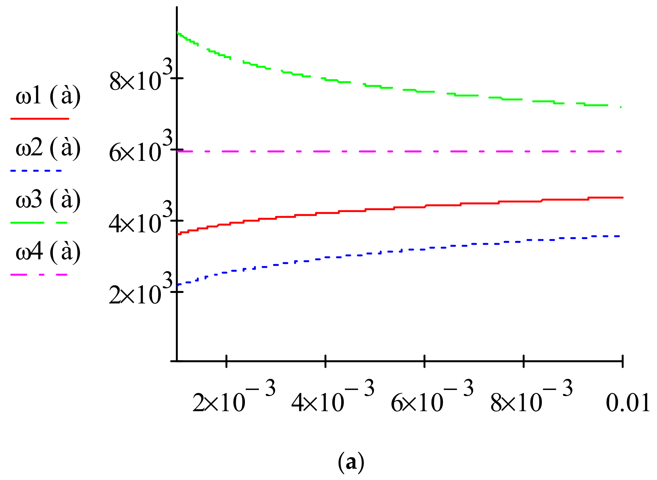
Abstract
1. Introduction
2. Mathematical Model of Longitudinal Oscillations of an Elastic Body under the Impulse Action of External Perturbation
- (a)
- from the periodicity of the perturbation follows
- (b)
- from the main properties of the function [22] it follows that with a sufficient degree of accuracy the pulse component of the external perturbation can be represented aswhere , and the lower parameter will be called the phase of external periodic perturbation.
3. Method of Constructing an Asymptotic Approximation of the Solution of a Mathematical Model of Nonlinear Oscillations of Elastic Body under Pulsed Action of Forces
- In the differential Equation (9) and below the indices which indicates the form of “dynamic equilibrium” of the elastic body for ease of recording omitted;
- Quantity according to the frequency of natural oscillations takes values ;
- Depending on the Equation (10) function based on the properties of the system of functions that describe the forms of oscillations of undisturbed motion are presented in the form .
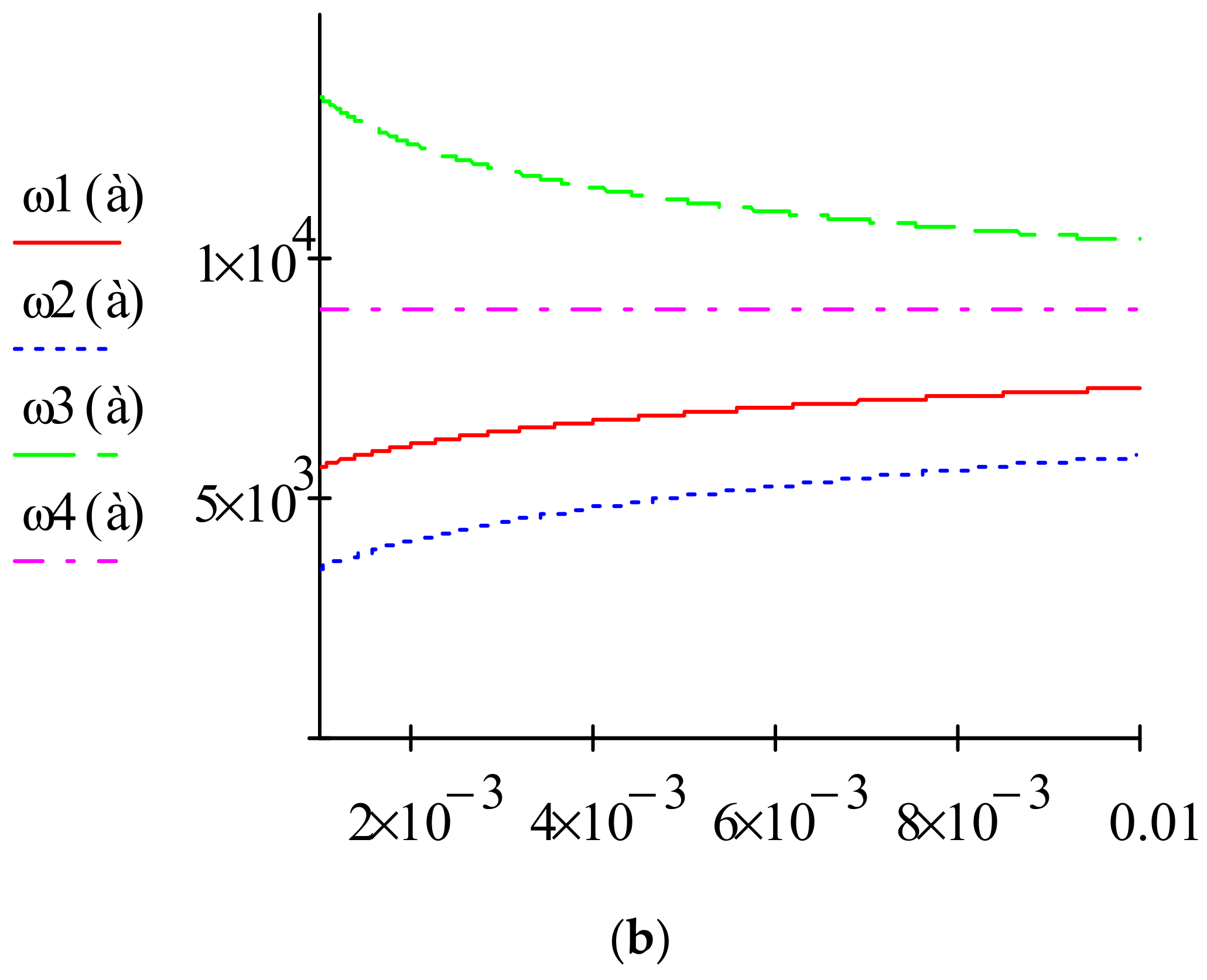
3.1. Amplitude-Frequency Characteristics of Non-Resonant Oscillations of an Elastic Body
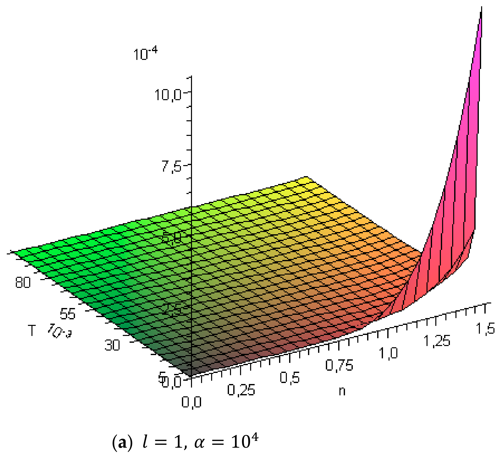
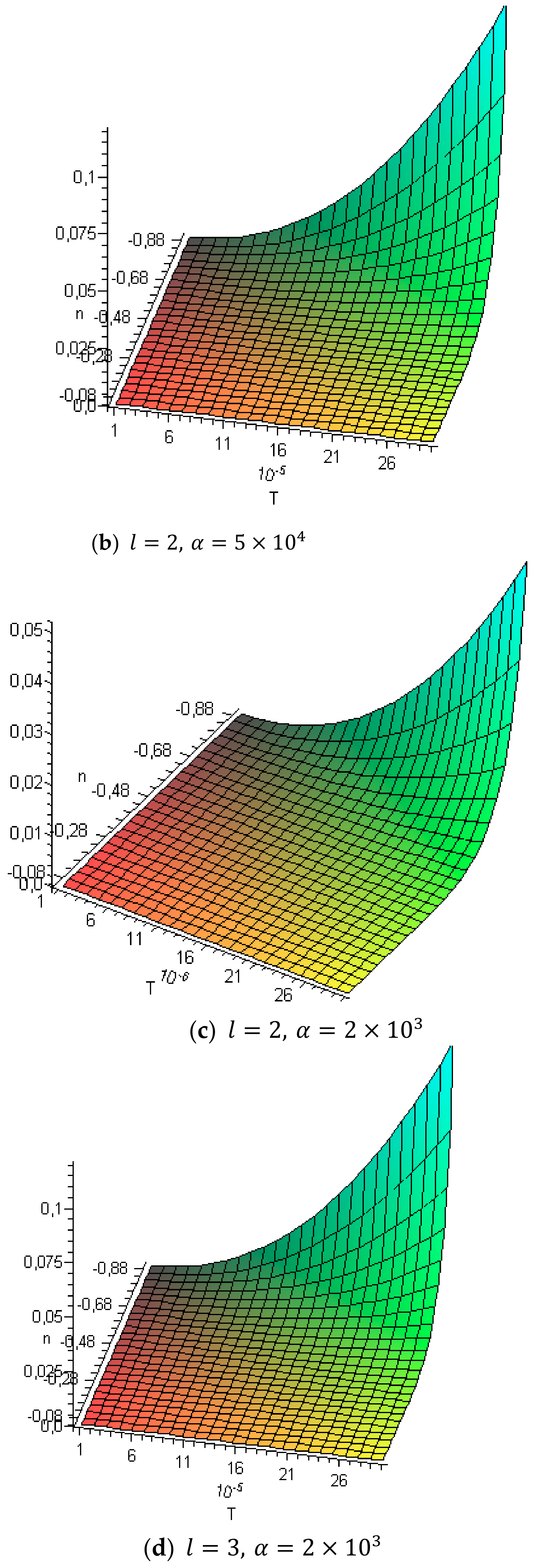
3.2. Resonant Oscillations of a Substantially Nonlinear Elastic Body under the Action of Periodic Impulse Forces
- First, the defining parameters that describe the dynamics of the process significantly depend on the “phase difference” natural oscillations and periodic perturbations;
- Secondly, it takes place under the condition that the amplitude of the process approaches the value ;
- Third, if the initial amplitude is less than , and function describes only dissipative and nonlinearly elastic forces, then a small periodic momentum perturbation can cause a resonant process in an elastic body cannot;
- Fourth, the main part of the speed of the “phase difference” for the case of transition through resonance, as follows from the above, can be presented as or .


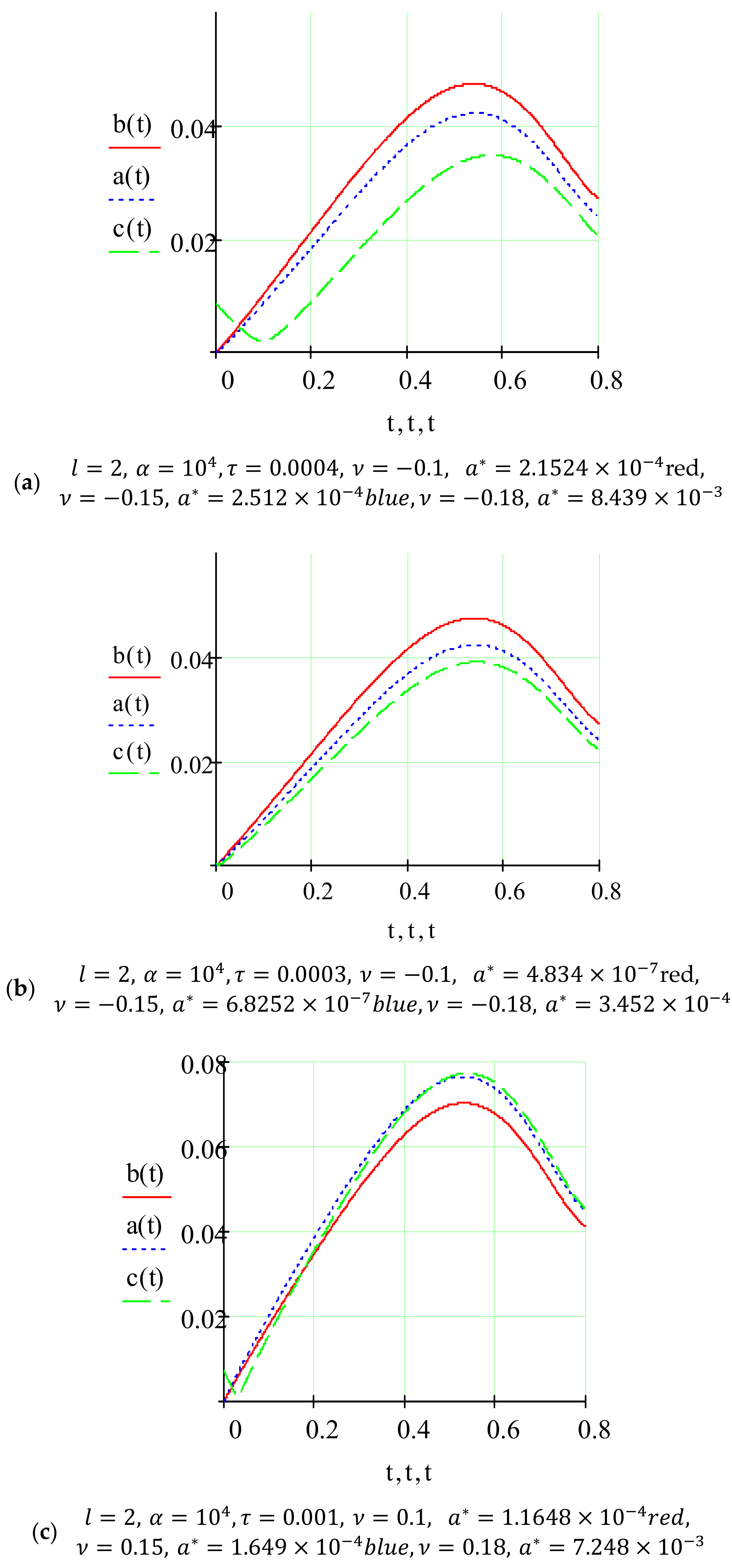
- for the case a smaller value of the specified parameter corresponds to a larger value of the resonant amplitude and at the same time the amplitude of the passage through the resonance is smaller;
- for the case its larger value corresponds to a larger value of the resonant amplitude and at the same time the amplitude of the resonance is larger;
- for the case a smaller value of the pulse perturbation frequency corresponds to a smaller value of the resonant amplitude and a larger value of the amplitude of the passage through the resonance.
4. Conclusions
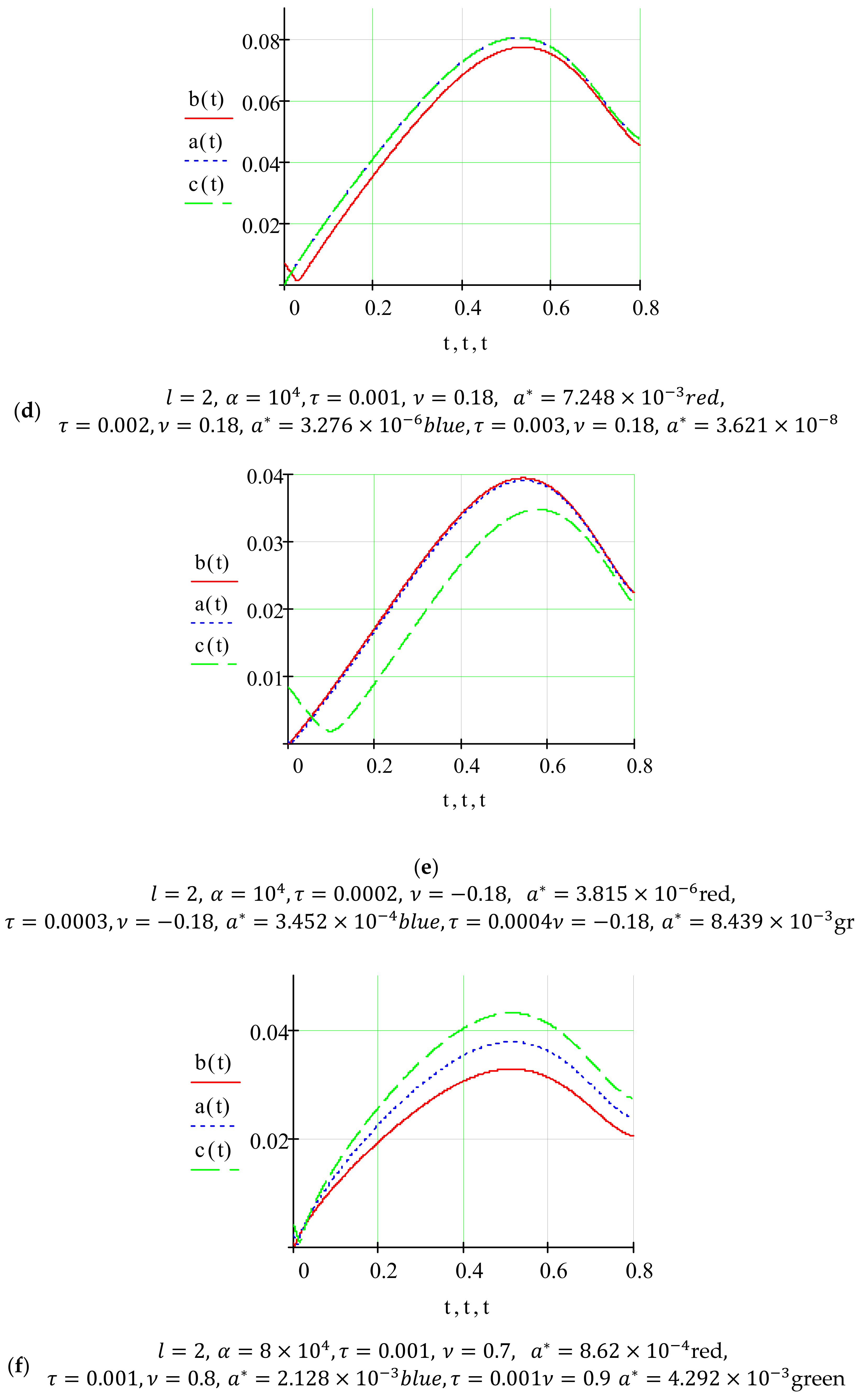
- for a constant value of periodic pulsed perturbation, the amplitude of the passage through the main resonance for the rigid elastic properties of bodies () for larger values of the pulse perturbation frequency takes larger values and vice versa for the soft elastic properties of bodies () a smaller value of the pulse perturbation frequency corresponds to a larger value of the amplitude of the passage through the resonance;
- the amplitude of the passage through the resonance depends on the point of application of the pulse perturbation and boundary conditions. In the case of an elastic body with fixed ends, the maximum value of the amplitude of passage through resonance will be for the case of impulse perturbation on the middle of the elastic body, and for an elastic body with free ends—for the case of impulse perturbation on the end of the elastic body.
Author Contributions
Funding
Institutional Review Board Statement
Informed Consent Statement
Data Availability Statement
Conflicts of Interest
References
- Pisarenko, G.S.; Kvitka, O.L.; Umansky, E.S. Resistance of Materials; Higher School: Kyiv, Ukraine, 2004; 655p, ISBN 966-642-056-2. [Google Scholar]
- Lott, D.A.; Antman, S.S.; Szymczak, W.G. The Quasilinear Wave Equation for Antiplane Shearing of Nonlinearly Elastic Bodies. J. Comput. Phys. 2001, 171, 201–226. [Google Scholar] [CrossRef]
- Habeck, D.; Schuricht, F. Contact between nonlinearly elastic bodies. Proc. R Soc. Edinb. Sect. A-Math. 2006, 136, 1239–1266. [Google Scholar] [CrossRef]
- Antman, S.; Shvartsman, M. The Shrink-Fit Problem for Aeolotropic Nonlinearly Elastic Bodies. J. Elast. 1995, 37, 157–166. [Google Scholar] [CrossRef]
- Annin, B.D.; Bondar, V.D. Antiplane Strain in a Nonlinearly Elastic Incompressible Body. J. Appl. Mech. Tech. Phys. 2006, 47, 849–856. [Google Scholar] [CrossRef]
- Warne, P.G.; Polignone, D.A. Solutions for an infinite compressible nonlinearly elastic body under a line load. Q. Appl. Math. 1996, 54, 317–326. [Google Scholar] [CrossRef]
- Kryvinska, N.; Bickel, L. Scenario-Based Analysis of IT Enterprises Servitization as a Part of Digital Transformation of Modern Economy. Appl. Sci. 2020, 10, 1076. [Google Scholar] [CrossRef]
- Tkachenko, R.; Izonin, I.; Kryvinska, N.; Dronyuk, I.; Zub, K. An Approach towards Increasing Prediction Accuracy for the Recovery of Missing IoT Data based on the GRNN-SGTM Ensemble. Sensors 2020, 20, 2625. [Google Scholar] [CrossRef] [PubMed]
- Cveticanin, L. Strong Nonlinear Oscillator—Analytical Solutions. In Mathematical Engineering; Springer International Publishing AG: New York, NY, USA, 2018; 317p. [Google Scholar] [CrossRef]
- Cveticanin, L. Period of vibration of axially vibrating truly nonlinear rod. J. Sound Vib. 2016, 374, 199–210. [Google Scholar] [CrossRef]
- Cveticanin, L.; Pogány, T. Oscillator with a Sum of Noninteger-Order Nonlinearities. J. Appl. Math. 2012, 2012, 1–20. [Google Scholar] [CrossRef]
- Gendelman, O.; Vakakis, A.F. Transitions from localization to nonlocalization in strongly nonlinear damped oscillators. Chaos, Solitons Fractals 2000, 11, 1535–1542. [Google Scholar] [CrossRef]
- Sokil, B.I.; Barvinskii, A.F. An asymptotic expansion for a class of nonlinear differential equations. Ukr. Math. J. 1981, 32, 465–468. [Google Scholar] [CrossRef]
- Sokil, B.I. Construction of asymptotic solutions of certain boundary-value problems for the nonautonomous wave equation. J. Math. Sci. 1999, 96, 2878–2882. [Google Scholar] [CrossRef]
- Pukach, P.Y. Qualitative Methods for the Investigation of a Mathematical Model of Nonlinear Vibrations of a Conveyer Belt. J. Math. Sci. 2014, 198, 31–38. [Google Scholar] [CrossRef]
- Antman, S.S.; Zhong-Heng, G. Large shearing oscillations of incompressible nonlinearly elastic bodies. J. Elast. 1984, 14, 249–262. [Google Scholar] [CrossRef]
- Myshkis, A.D.; Filimonov, A.M. Periodic oscillations in nonlinear one-dimensional continuous media. In Proceedings of the IX International Conference on Nonlinear Oscillations, Kyiv, Ukraine, 30 August–6 September 1981; Part 1, Analytical methods. Naukova Dumka: Kyiv, Ukraine, 1984; pp. 274–276. [Google Scholar]
- Erbay, H.A.; Erbay, S.; Erkip, A. The Cauchy problem for a class of two-dimensional nonlocal nonlinear wave equations governing anti-plane shear motions in elastic materials. Nonlinearity 2011, 24, 1347–1359. [Google Scholar] [CrossRef]
- Räty, R.; Von Boehm, J.; Ranta, M. Non-linearly Forced Vibrations of Elastic Systems Carrying Rigid Bodies. J. Sound Vib. 1994, 169, 71–87. [Google Scholar] [CrossRef]
- Delta Function. Mathematics. Available online: https://mathworld.wolfram.com/DeltaFunction.html (accessed on 20 July 2020).
- Zelenina, A.; Zubov, L.M. One-dimensional deformations of nonlinearly elastic micropolar bodies. Mech. Solids 2010, 45, 575–582. [Google Scholar] [CrossRef]
- Liu, X.Q.; Ni, X.H.; Ma, Y.C. Elastic-plastic analysis of nonlinearly elastic structure in the space bars pinned on a rigid body. In Proceedings of the 4th International Symposium on Test and Measurement, Shanghai, China, 1–3 June 2001; Chinese Society of Modern Technical Equipments: Shanghai, China, 2001; Volume 1–2, pp. 1084–1086. [Google Scholar]
- Cattani, C.; Rushchitskii, Y.Y. The subharmonic resonance and second harmonic of a plane wave in nonlinearly elastic bodies. Int. Appl. Mech. 2003, 39, 93–98. [Google Scholar] [CrossRef]
- Andrukhiv, A.; Sokil, M.; Fedushko, S.; Syerov, Y.; Kalambet, Y.; Peracek, T. Methodology for Increasing the Efficiency of Dynamic Process Calculations in Elastic Elements of Complex Engineering Constructions. Electronics 2021, 10, 40. [Google Scholar] [CrossRef]
- Ni, X.H.; Liu, X.Q.; Lu, X.B. The stress-strain analysis of the nonlinearly elastic structure of the bars pinned to a turntable rigid body. In Proceedings of the 4th International Symposium on Test and Measurement, Shanghai, China, 1–3 June 2001; Chinese Society of Modern Technical Equipments: Shanghai, China, 2001; Volume 1–2, pp. 1039–1040. [Google Scholar]


Publisher’s Note: MDPI stays neutral with regard to jurisdictional claims in published maps and institutional affiliations. |
© 2021 by the authors. Licensee MDPI, Basel, Switzerland. This article is an open access article distributed under the terms and conditions of the Creative Commons Attribution (CC BY) license (https://creativecommons.org/licenses/by/4.0/).
Share and Cite
Andrukhiv, A.; Sokil, M.; Sokil, B.; Fedushko, S.; Syerov, Y.; Karovic, V., Jr.; Klynina, T. Influence of Impulse Disturbances on Oscillations of Nonlinearly Elastic Bodies. Mathematics 2021, 9, 819. https://doi.org/10.3390/math9080819
Andrukhiv A, Sokil M, Sokil B, Fedushko S, Syerov Y, Karovic V Jr., Klynina T. Influence of Impulse Disturbances on Oscillations of Nonlinearly Elastic Bodies. Mathematics. 2021; 9(8):819. https://doi.org/10.3390/math9080819
Chicago/Turabian StyleAndrukhiv, Andriy, Mariia Sokil, Bohdan Sokil, Solomiia Fedushko, Yuriy Syerov, Vincent Karovic, Jr., and Tetiana Klynina. 2021. "Influence of Impulse Disturbances on Oscillations of Nonlinearly Elastic Bodies" Mathematics 9, no. 8: 819. https://doi.org/10.3390/math9080819
APA StyleAndrukhiv, A., Sokil, M., Sokil, B., Fedushko, S., Syerov, Y., Karovic, V., Jr., & Klynina, T. (2021). Influence of Impulse Disturbances on Oscillations of Nonlinearly Elastic Bodies. Mathematics, 9(8), 819. https://doi.org/10.3390/math9080819