Mathematical and Statistical Analysis of Doubling Times to Investigate the Early Spread of Epidemics: Application to the COVID-19 Pandemic

Abstract

Simple mathematical tools are needed to quantify the threat posed by emerging and re-emerging infectious disease outbreaks using minimal data capturing the outbreak trajectory. Here we use mathematical analysis, simulation and COVID-19 epidemic data to demonstrate a novel approach to numerically and mathematically characterize the rate at which the doubling time of an epidemic is changing over time. For this purpose, we analyze the dynamics of epidemic doubling times during the initial epidemic stage, defined as the sequence of times at which the cumulative incidence doubles. We introduce new methodology to characterize epidemic threats by analyzing the evolution of epidemics as a function of (1) the number of times the epidemic doubles until the epidemic peak is reached and (2) the rate at which the doubling times increase. In our doubling-time approach, the most dangerous epidemic threats double in size many times and the doubling times change at a relatively low rate (e.g., doubling times remain nearly invariant) whereas the least transmissible threats double in size only a few times and the doubling times rapidly increases in the period of emergence. We derive analytical formulas and test and illustrate our methodology using synthetic and COVID-19 epidemic data. Our mathematical analysis demonstrates that the series of epidemic doubling times increase approximately according to an exponential function with a rate that quantifies the rate of change of the doubling times. Our analytic results are in excellent agreement with numerical results. Our methodology offers a simple and intuitive approach that relies on minimal outbreak trajectory data to characterize the threat posed by emerging and re-emerging infectious diseases.

1. Introduction

The trajectory of an infectious disease epidemic, which is typically tracked as the number of new reported cases by date of symptoms onset, is shaped by multiple factors including the natural history of the disease, background immunity patterns, environmental factors [1], superspreading events [2], control interventions and behavior changes. These factors are not static but change over the different time scales associated with the natural history of the infectious disease (e.g., influenza, Ebola, HIV/AIDS). Further, these factors shape the early growth dynamics [3,4] and the basic reproduction number ($R_0$), which quantifies the number of secondary cases per primary case in a completely susceptible population, and the generation interval, which dictates the time scale for the generation of new cases [5]. It is worth pointing out that even the generation interval is not necessarily invariant, but it can be affected during the course of an outbreak by control interventions and susceptible depletion (e.g., contact tracing and isolation) [6,7]. Hence, transmission estimates that capture dynamic changes in epidemic growth could provide a conceptual framework to characterize the epidemic threat posed by infectious diseases.

Parameter $R_0$ is a widely used indicator of transmission potential in a native population and is driven by the average contact rate and the mean infectious period of the disease [5]. Yet, it only characterizes transmission potential at the onset of the epidemic and varies geographically for a given infectious disease according to local healthcare, outbreak response, social, and cultural factors that in turn influence the probability of superspreading events [8,9,10]. Furthermore, estimating $R_0$ requires information about the natural history of the infectious disease. Thus, our ability to estimate reproduction numbers for novel infectious diseases is hindered by the lack of information about their epidemiological characteristics and transmission mechanisms. Therefore, approaches that rely on empirical patterns rather than specific mechanistic assumptions have proved valuable especially during the early transmission stages [11]. It is also worth noting that mathematical analyses of the doubling time of epidemics remain limited to exponentially growing epidemics, an assumption that does not always hold. Here we derive and demonstrate mathematical expressions that allow the characterization of the rate of change of the doubling time beyond exponential growth dynamics.

Although the effective reproduction number, $R_t$, tracks time-dependent changes in transmission potential during the course of an epidemic, this quantity does not convey information about the magnitude or dynamic changes in the trajectory of the epidemic [12]. For instance, $R_t$ could be fluctuating over time around the epidemic threshold of 1.0 regardless of whether the outbreak’s incidence rate is fluctuating around tens of cases per week or fluctuating around thousands of cases per week. This is because epidemic trajectories at broader spatial scales hide sub-epidemic growth dynamics. More informative metrics could synthesize real-time information about the extent to which the epidemic is expanding over time. Such metrics would be particularly useful if they rely on minimal data, such as time series of cases or deaths, of the outbreak’s trajectory.

Epidemic doubling times characterize the sequence of times at which the cumulative incidence doubles [13,14,15,16,17,18]. Here we introduce metrics that capture the dynamics of epidemic doubling times to provide a parsimonious and practical framework to quantify the threat associated with infectious diseases. We use mathematical and numerical analysis which we illustrate using COVID-19 epidemic data of the early stages of the epidemic in various hotspot countries.

2. Data Sources

2.1. Representative Country-Level COVID-19 Data

We retrieved daily reported cumulative case data of the early spread of the COVID-19 pandemic in Germany, France, Canada, the United Kingdom (UK), The Netherlands, and the United States of America (USA) from the World Health Organization (WHO) website [19] and for Spain and Italy from the corresponding governmental datasets [20,21] from early February to 24 May 2020. We calculated the daily incidence from the cumulative trajectory and analyzed the early incidence trajectory for the 8 countries.

2.2. Synthetic Epidemic Growth Data

We conducted simulation studies for testing and demonstrating the mathematical results and estimation of parameters characterizing the rate of change of doubling times. For this purpose, we simulated epidemic growth curves by adding a Poisson error structure to the daily incidence curve obtained from the generalized-growth model (GGM) [8,22], which provides a first approximation to the growth phase of the epidemic’s trajectory. We generate synthetic data to verify the methodology before we apply it to real epidemic data.

3. The Generalized-Growth Model for Early Ascending Phase

We analyze the evolution of epidemics as a function of the number of times the cumulative incidence doubles before the epidemic peaks, and the rate at which the doubling time increases (hence the epidemic slows down), owing to interventions, behavior changes and depletion of susceptible individuals. The most difficult to control are epidemic threats that double in size many times by the time the peak has been reached, while doubling times increase at a relatively low rate. Conversely, the least difficult to control are epidemic threats that only double in size very few times, while the sequence of doubling times rapidly increases.

During the epidemic growth phase, the times at which cumulative incidence doubles are given by $t_i$ such that $2C\left(t_i\right)=C\left(t_{i+1}\right)$, where $t_0=0$, $C\left(t_0\right)=C_0$, $i=0,1\dots ,n_d-1$, and $n_d$ is the total number of times cumulative incidence doubles (Figure 1A). The actual sequence of “doubling times” is defined as follows (see Figure 1B):

$$\Delta t_j=t_j-t_{j-1},\mathrm{where}j=1,\dots ,n_d.$$

As a first approximation, we employ the generalized-growth model (GGM) [8,22] to characterize the temporal evolution of doubling times during the growth phase of the epidemic’s trajectory. The GGM is a useful phenomenological model that relaxes the assumption of exponential growth in the early ascending phase of an outbreak, taking the form:

$$C^{\prime }=r{C}^p\left(t\right),$$

(1)

where $C^{\prime }\left(t\right)$ describes the incidence at time t, the solution $C\left(t\right)$ describes the cumulative number of cases at time t, r is a positive parameter denoting the growth rate (with units of (people)${}^{(1-p)}$ per time), and $p\in [0,1]$ is a “deceleration of growth” parameter (dimensionless). If $p=0$, this equation describes constant incidence over time and the cumulative number of cases grows linearly, whereas $p=1$ describes exponential growth. This model has been shown to provide an improved description of the early growth phase of epidemics [8,22] and has displayed promising results for short-term epidemic forecasting [23,24,25].

For exponential growth dynamics (i.e., $p=1$), it is well known that the doubling times remain invariant and is given by: $\Delta t_j=\frac{ln2}{r}$, whereas the doubling times follow an increasing trend when the epidemic grows sub-exponentially fast as shown in Figure 1.

When $p<1$ (sub-exponential epidemic growth), given a time $t>0$ and the initial number of cases $C_0$, one can determine the time to the doubling of cases from t. That is, given $t>0$, one can find $\Delta t=\Delta t\left(t\right)$ such that $2C\left(t\right)=C(t+\Delta t)$. As shown in the next section, this function is given by

$$\Delta t=\left(2^{1-p}-1\right)\left\{t+\frac{C_0^{1-p}}{(1-p)r}\right\}.$$

(2)

Alternatively, one can also express the doubling time $\Delta t$ as a function of $C=C\left(t\right)$ as follows (full derivation given below):

$$\Delta t=\left(2^{1-p}-1\right)\frac{C^{1-p}\left(t\right)}{(1-p)r}.$$

(3)

Thus, for the case of sub-exponential growth, i.e., when $p<1$, one concludes that the doubling time increases exponentially according to

$$\Delta t_{j+1}=\lambda {\mathrm{e}}^{b_{d}j},b_d:=(1-p)ln2,\lambda :=\frac{\left(2^{1-p}-1\right)C_0^{1-p}}{(1-p)r},j=0,1,2\dots .$$

(4)

The constant $b_d$ depends only on the deceleration of growth parameter $p<1$. Hence, $b_d$ is the exponential rate at which the doubling times, $\Delta t_j$, increase. The slower the rate $b_d$, the slower the rate at which the epidemic doubling times increase, which tends to increase the number of times the epidemic doubles.

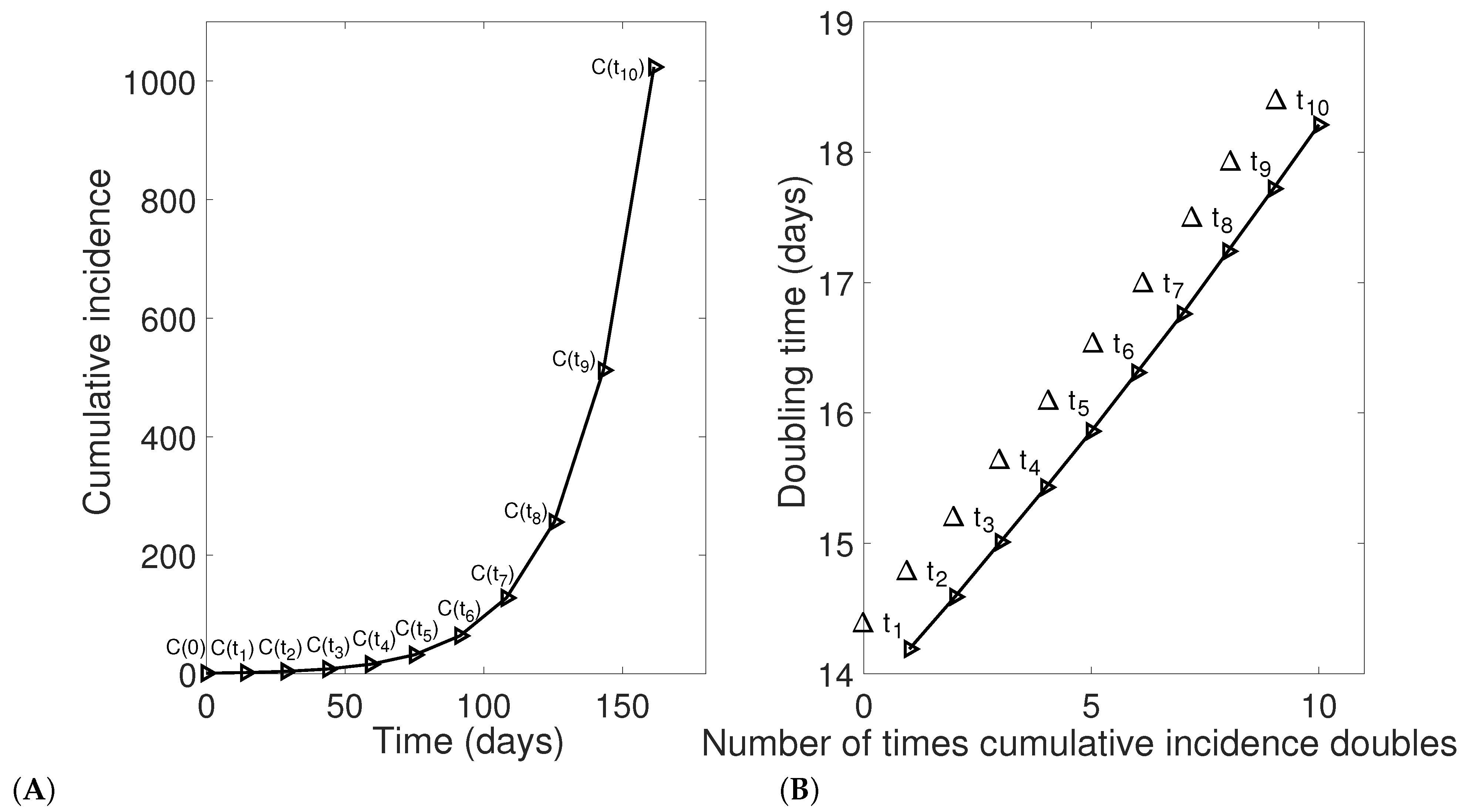
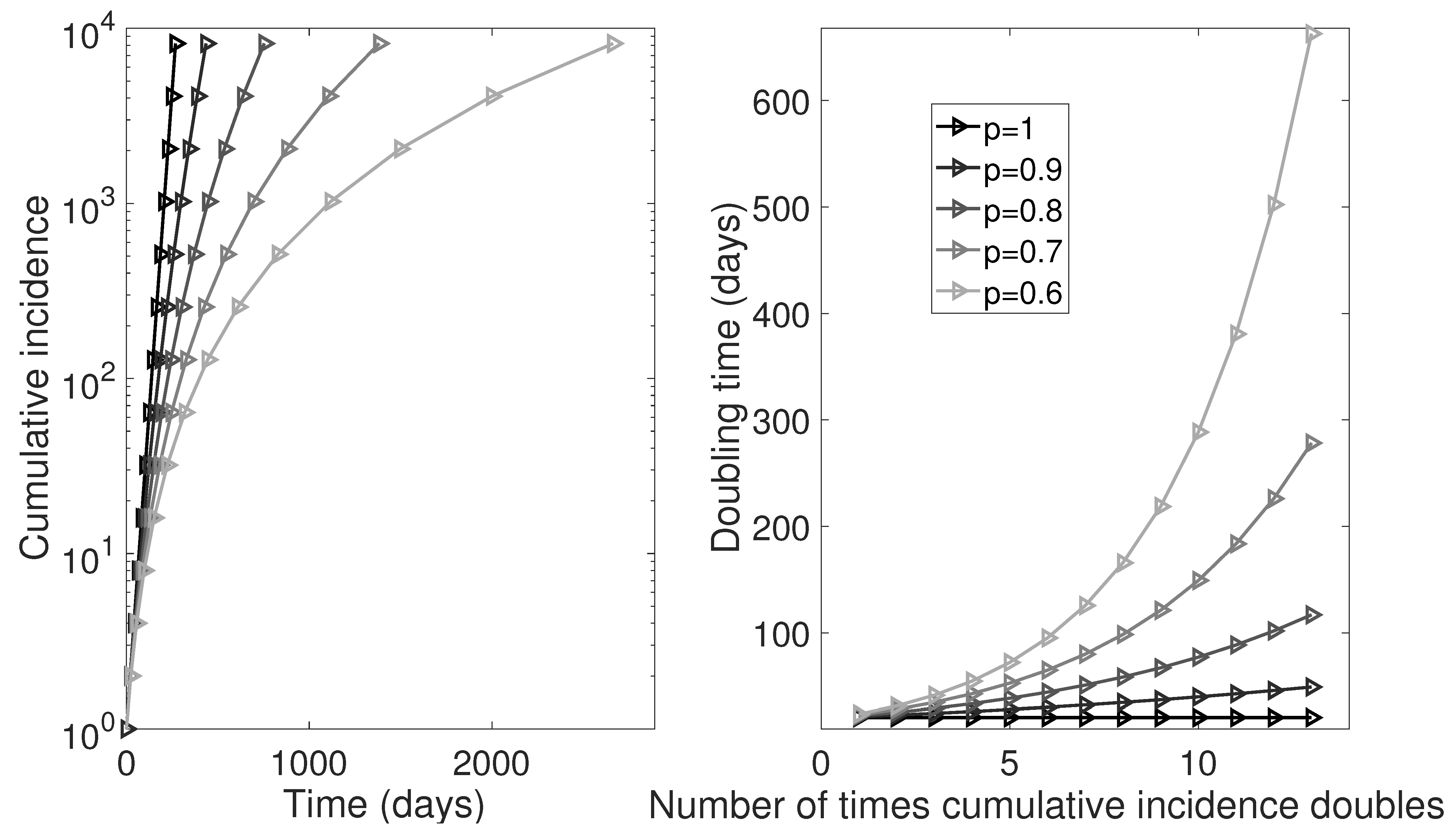
4. Evolution of Doubling Times for Sub-Exponential Growth. Mathematical Analysis

In this section, we carry out mathematical analysis of the temporal evolution of doubling times during the epidemic growth phase using the generalized growth model (1). We wish to find the “doubling time”, $\Delta t$, such that for any $t>0$,

$$2C\left(t\right)=C(t+\Delta t).$$

(5)

For exponential growth dynamics (i.e., $p=1$), one can easily check that $\Delta t$ remains invariant and is given by $\Delta t=\frac{ln2}{r}.$ Consider the case $p<1$ (sub-exponential epidemic growth). Given $C\left(0\right)=C_0$, from Equation (1) one obtains

$$C\left(t\right)={\left\{(1-p)rt+C_0^{1-p}\right\}}^{\frac{1}{1-p}}.$$

(6)

Substituting expression (6) into (5), one has

$$2{\left\{(1-p)rt+C_0^{1-p}\right\}}^{\frac{1}{1-p}}={\left\{(1-p)r(t+\Delta t)+C_0^{1-p}\right\}}^{\frac{1}{1-p}}.$$

(7)

This identity is equivalent to

$$2^{1-p}\left\{(1-p)rt+C_0^{1-p}\right\}=(1-p)r(t+\Delta t)+C_0^{1-p}.$$

(8)

In order to solve for $\Delta t$, we rewrite (8) as

$$2^{1-p}\left\{(1-p)rt+C_0^{1-p}\right\}-\left\{(1-p)rt+C_0^{1-p}\right\}=(1-p)r\Delta t.$$

(9)

Equation (9) yields

$$\left(2^{1-p}-1\right)\left\{(1-p)rt+C_0^{1-p}\right\}=(1-p)r\Delta t,$$

(10)

and therefore

$$\Delta t=\frac{\left(2^{1-p}-1\right)\left\{(1-p)rt+C_0^{1-p}\right\}}{(1-p)r}=\left(2^{1-p}-1\right)\left\{t+\frac{C_0^{1-p}}{(1-p)r}\right\}.$$

(11)

This proves (2) as stated in Section 3 above. One can also express the doubling time, $\Delta t$, as a function of $C\left(t\right)$. Indeed, according to (6),

$$C^{1-p}\left(t\right)=(1-p)rt+C_0^{1-p}.$$

(12)

Identity (12) implies

$$t=\frac{C^{1-p}\left(t\right)-C_0^{1-p}}{(1-p)r}.$$

(13)

Combining (11) and (13), one concludes

$$\Delta t=\left(2^{1-p}-1\right)\left\{\frac{C^{1-p}\left(t\right)-C_0^{1-p}}{(1-p)r}+\frac{C_0^{1-p}}{(1-p)r}\right\}=\left(2^{1-p}-1\right)\frac{C^{1-p}\left(t\right)}{(1-p)r}.$$

(14)

Thus, given $C\left(t\right)$, r and p, we can determine $\Delta t$. This confirms property (3) of sub-exponential growth model introduced in Section 3.

Consider the sequence of doubling times, $\{\Delta t_j\}$, $j=0,1,2\dots$, such that

$$\Delta t_0:=0,2C\left(\sum _{k=0}^j\Delta t_k\right)=C\left(\sum _{k=0}^{j+1}\Delta t_k\right).$$

(15)

Importantly, for the case of sub-exponential growth, i.e., when $p<1$, one can verify that $\{\Delta t_j\}$ increases exponentially according to:

$$\Delta t_{j+1}=\lambda {\mathrm{e}}^{bj},b:=(1-p)ln2,\lambda :=\frac{\left(2^{1-p}-1\right)C_0^{1-p}}{(1-p)r},j=0,1,2\dots .$$

(16)

To verify (16), set $\alpha :=2^{1-p}-1$. It follows from (11) that

$$\Delta t_{j+1}=\left(2^{1-p}-1\right)\left\{\sum _{k=0}^j\Delta t_k+\frac{C_0^{1-p}}{(1-p)r}\right\}=\alpha \sum _{k=0}^j\Delta t_k+\lambda .$$

(17)

Specifically, by (15) and (17) one has

$$\Delta t_0=0,\Delta t_1=\lambda ,$$

(18)

$$\Delta t_2=\alpha \Delta t_1+\lambda =\lambda (\alpha +1),$$

(19)

$$\Delta t_3=\alpha (\Delta t_1+\Delta t_2)+\lambda =\lambda {(\alpha +1)}^2,\dots$$

(20)

$$\Delta t_{j+1}=\lambda {(\alpha +1)}^j=\lambda {\left(2^{1-p}-1+1\right)}^j=\lambda 2^{j(1-p)}=\lambda {\mathrm{e}}^{j(1-p)ln2},$$

(21)

which completes the proof.

5. Simulation Studies to Verify Analytic Results

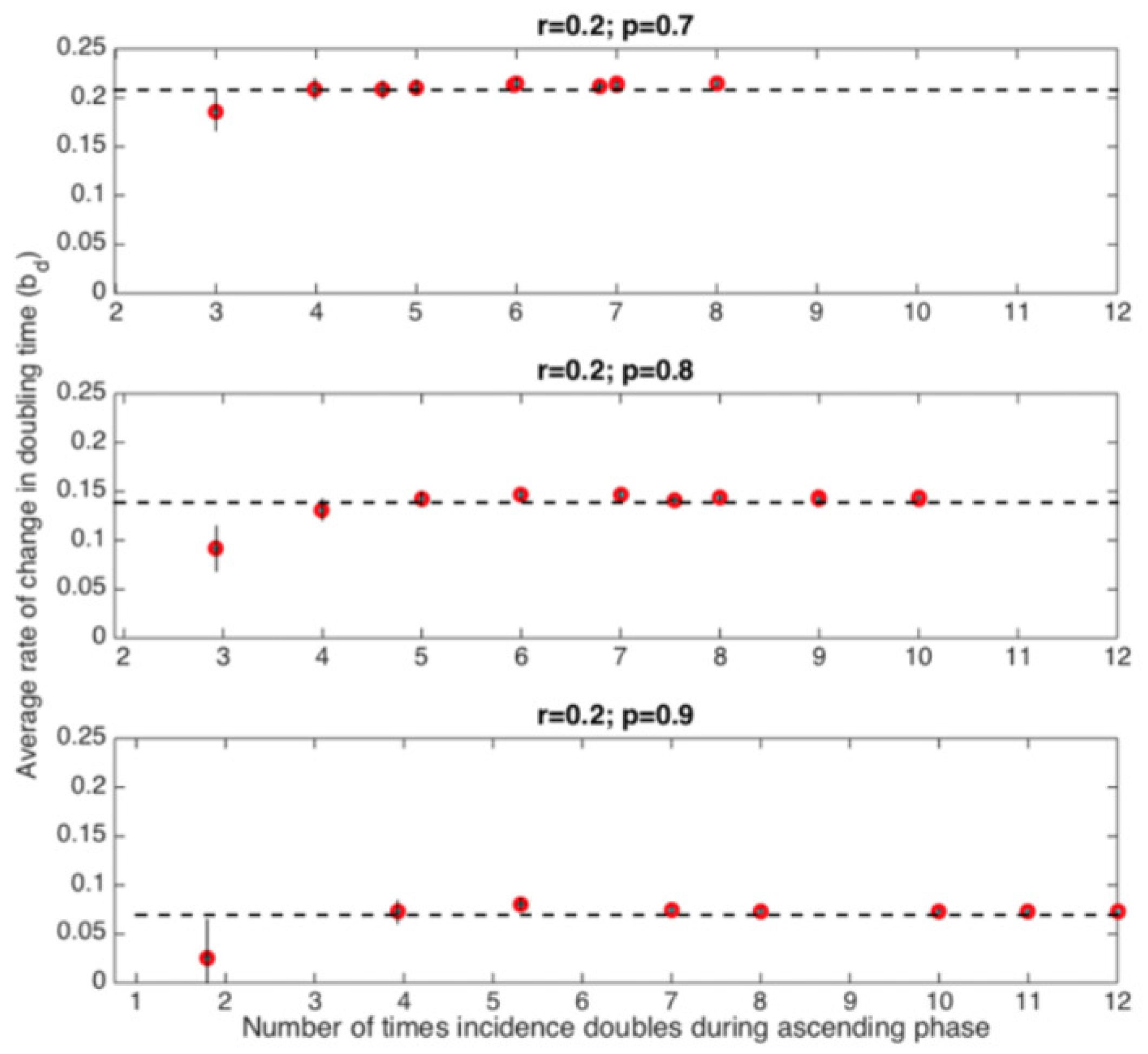
5.1. Estimating the Rate of Change of Doubling Times from Epidemic Data

The exponential rate, $b_d$, at which the doubling times $\Delta t_j$ increase can simply be estimated by least squares fitting, where we estimate $b_d$ as the slope of the line given by the equation:

$$ln(\Delta t_j)=ln\left(\frac{\lambda }{\alpha +1}\right)+b_{d}j.$$

The intercept parameter, $ln\left(\frac{\lambda }{\alpha +1}\right)$, is also estimated using least squares. That is, we estimate two parameters denoted by $\Theta$, and the sequence of doubling times given by $\Delta t_j$ is sufficient to estimate both.

To quantify parameter uncertainty, we employ parametric bootstrapping with a Poisson error structure (e.g., [26,27,28]) around the incidence curve from which the sequence of doubling times, $\Delta t_j$, can be obtained. That is, we re-estimate parameters ${\Theta }_i$, where $i=1,2,\dots ,s$, and s is the number of bootstrap realizations.

5.2. Doubling Time Analysis of COVID-19 Epidemics

We conducted simulation studies to verify our analytic results and assess the amount of time-series data (e.g., number of doublings in cumulative incidence) that is needed to reliably estimate the rate $b_d$ at which the doubling times increase. For this purpose, we simulated 500 incidence curves comprising 35 days by adding a Poisson error structure to the daily incidence curve obtained from the generalized-growth model. For illustration, we set common parameter $r=0.2$ and vary the scaling of growth parameter, p. The initial condition was set at $C\left(0\right)=1$, see Figure 2.

Figure 3 shows that the analytic results of the rate of change of doubling times, $b_d$, are consistent with our numerical results (Figure 3B). We also assessed our ability to estimate $b_d$ from limited simulated data using the GGM that incorporates a Poisson error structure as described above. Our results based on simulated data indicate that the parameter $b_d$ can be reliably estimated from the first few doubling times of the epidemic (Figure 4).

The evolution of the doubling times during the early phase of the representative COVID-19 epidemics in various hotspot countries is displayed in Figure 5. Overall, the mean doubling time ranged from 1.9 (Italy) to 4.1 (Canada). Importantly, Figure 5 also shows that the sequence of doubling times is well characterized by the generalized-growth model.

6. Conclusions

In this paper, we have introduced a novel framework to characterize epidemic control based on the evolution of doubling times associated with the epidemic’s ascending phase. Our methodology, based on analytic and numerical results, validated by simulations, relies on minimal outbreak data and, is independent of the time scales driving the transmission process. Our work contributes in several ways:

(1)

Our approach provides a framework to numerically and mathematically characterize the rate at which the doubling time of an epidemic is changing over time.

(2)

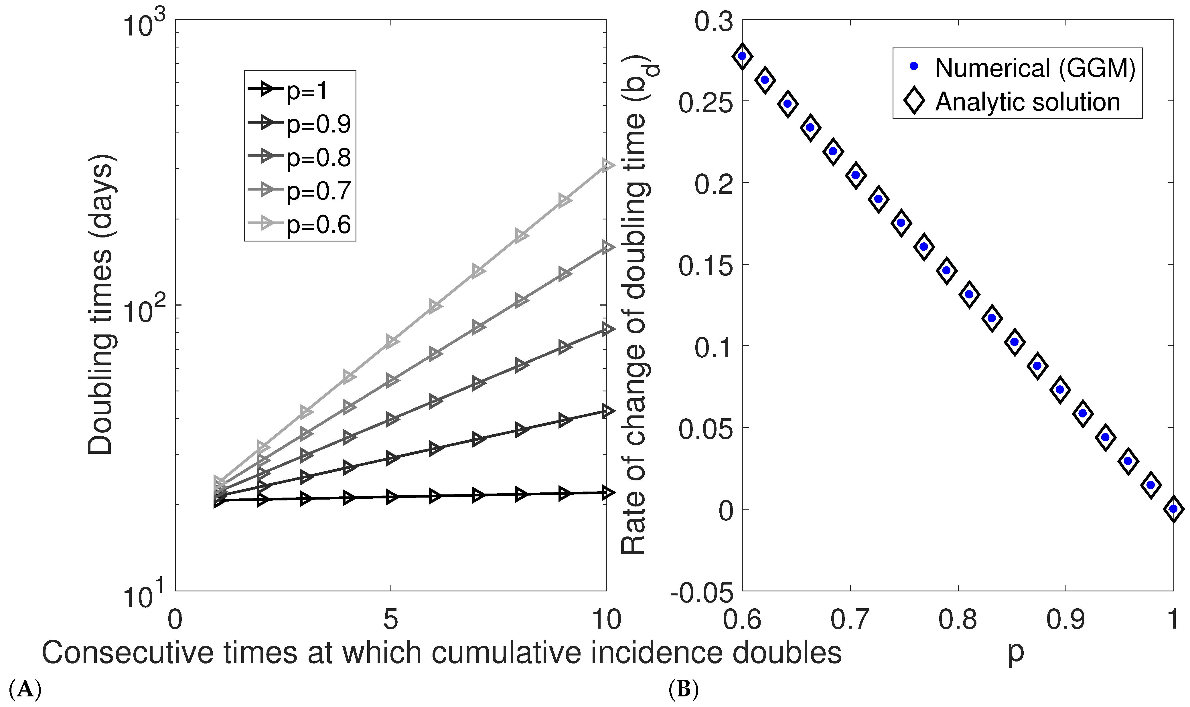
We derive analytical formulas of the rate at which the doubling time is changing and test and illustrate our methodology using synthetic and COVID-19 epidemic data.

(3)

Our mathematical analysis (and proof) demonstrates that the series of epidemic doubling times increase approximately according to an exponential function with a rate that quantifies the rate of change of the doubling times. Our analytic results are in excellent agreement with numerical simulations.

Future studies could characterize the doubling times for past outbreaks of different infectious diseases at different geographic and spatial contexts in order to glean a more refined and comprehensive picture of the relationship between changing doubling times and geographic variability in socio-demographic factors and interventions. Indeed, all outbreaks are influenced by stochasticity and by multiple factors including the mode of transmission and severity that shapes the transmission network structure as well as the fraction of the susceptible population [3,29,30,31,32] and the effects of behavior changes and control interventions [3,33,34].

Our analysis is not exempt of limitations. First, to illustrate our methodology we were not exhaustive on the number of outbreak datasets on COVID-19, but rather we focused on a convenient sample of COVID-19 datasets at the country level to illustrate our methodology. Second, surveillance epidemiological data is often subject to limitations. In particular, near real-time epidemiological data is often subject to measurement noise and reporting delays, in particular owing to the interval between infection and reporting [17]. Reporting delays could distort the incidence pattern particularly for the most recent weeks of the trajectory of the epidemic [35,36,37].

Our framework is based on a transmission scale that goes beyond estimates of transmission potential tied to the early epidemic onset such as $R_0$, or parameters such as Reff that does not include notions of outbreak magnitude. Our method could be readily applied for monitoring the progression of newly emerging or re-emerging infectious diseases as it only requires incidence data describing the cumulative number of cases as a function of time. However, as other transmission metrics, it may be affected by changes in case definitions or underreporting over the course of epidemics, particularly as epidemiological surveillance systems tend to capture more severe cases.

References

1. Weiss, R.A.; McMichael, A.J. Social and environmental risk factors in the emergence of infectious diseases. Nat. Med. 2004, 10, S70–S76. [Google Scholar] [CrossRef]
2. Lloyd-Smith, J.O.; Schreiber, S.J.; Kopp, P.E.; Getz, W.M. Superspreading and the effect of individual variation on disease emergence. Nat. Cell Biol. 2005, 438, 355–359. [Google Scholar] [CrossRef]
3. Szendroi, B.; Csnyi, G. Polynomial epidemics and clustering in contact networks. Proc. R. Soc. Lond. Ser. Biol. Sci. 2004, 271 (Suppl. S5), S364–S366. [Google Scholar] [CrossRef] [PubMed] [Green Version]
4. Chowell, G.; Viboud, C.; Hyman, J.M.; Simonsen, L. The Western Africa Ebola Virus Disease Epidemic Exhibits Both Global Exponential and Local Polynomial Growth Rates. PLoS Curr. 2014, 7, 7. [Google Scholar] [CrossRef]
5. Anderson, R.M.; May, R.M. Infectious Diseases of Humans; Oxford University Press: Oxford, UK, 1991. [Google Scholar]
6. Kenah, E.; Lipsitch, M.; Robins, J.M. Generation interval contraction and epidemic data analysis. Math. Biosci. 2008, 213, 71–79. [Google Scholar] [CrossRef] [PubMed] [Green Version]
7. Gostic, K.M.; McGough, L.; Baskerville, E.B.; Abbott, S.; Joshi, K.; Tedijanto, C.; Kahn, R.; Niehus, R.; Hay, J.A.; De Salazar, P.M.; et al. Practical considerations for measuring the effective reproductive number, Rt. PLoS Comput. Biol. 2020, 16, e1008409. [Google Scholar] [CrossRef]
8. Chowell, G.; Viboud, C.; Simonsen, L.; Moghadas, S.M. Characterizing the reproduction number of epidemics with early sub-exponential growth dynamics. J. R. Soc. Interface 2016, 13. [Google Scholar] [CrossRef] [Green Version]
9. Muniz-Rodriguez, K.; Fung, I.C.-H.; Ferdosi, S.R.; Ofori, S.K.; Lee, Y.; Tariq, A.; Chowell, G. Severe Acute Respiratory Syndrome Coronavirus 2 Transmission Potential, Iran, 2020. Emerg. Infect. Dis. 2020, 26, 1915–1917. [Google Scholar] [CrossRef] [PubMed]
10. Shim, E.; Tariq, A.; Chowell, G. Spatial variability in reproduction number and doubling time across two waves of the COVID-19 pandemic in South Korea, February to July, 2020. Int. J. Infect. Dis. 2021, 102, 1–9. [Google Scholar] [CrossRef]
11. Roosa, K.; Lee, Y.; Luo, R.; Kirpich, A.; Rothenberg, R.; Hyman, J.; Yan, P.; Chowell, G. Real-time forecasts of the COVID-19 epidemic in China from February 5th to February 24th, 2020. Infect. Dis. Model. 2020, 5, 256–263. [Google Scholar] [CrossRef]
12. Nishiura, H.; Chowell, G. The effective reproduction number as a prelude to statistical estimation of time-dependent epidemic trends. In Mathematical and Statistical Estimation Approaches in Epidemiology; Chowell, G., Hyman, J.M., Bettencourt, L.M.A., Castillo-Chavez, C., Eds.; Springer: Dordrecht, The Netherlands, 2009; pp. 103–121. [Google Scholar]
13. Muniz-Rodriguez, K.; Chowell, G.; Cheung, C.-H.; Jia, D.; Lai, P.-Y.; Lee, Y.; Liu, M.; Ofori, S.K.; Roosa, K.M.; Simonsen, L.; et al. Doubling Time of the COVID-19 Epidemic by Province, China. Emerg. Infect. Dis. 2020, 26, 1912–1914. [Google Scholar] [CrossRef] [PubMed]
14. Yan, P.; Chowell, G. Quantitative Methods for Investigating Infectious Disease Outbreaks; Springer: Cham, Switzerland, 2019. [Google Scholar]
15. Anderson, R.M.; Medley, G.F. Epidemiology of HIV infection and AIDS: Incubation and infectious periods, survival and vertical transmission. AIDS 1988, 2 (Suppl. S1), 57–63. [Google Scholar] [CrossRef]
16. Galvani, A.P.; Lei, X.; Jewell, N.P. Severe Acute Respiratory Syndrome: Temporal Stability and Geographic Variation in Case-Fatality Rates and Doubling Times. Emerg. Infect. Dis. 2003, 9, 991–994. [Google Scholar] [CrossRef]
17. Betensky, R.A.; Feng, Y. Accounting for incomplete testing in the estimation of epidemic parameters. Int. J. Epidemiol. 2020, 49, 1419–1426. [Google Scholar] [CrossRef] [PubMed]
18. Fung, I.C.-H.; Zhou, X.; Cheung, C.-N.; Ofori, S.K.; Muniz-Rodriguez, K.; Cheung, C.-H.; Lai, P.-Y.; Liu, M.; Chowell, G. Assessing Early Heterogeneity in Doubling Times of the COVID-19 Epidemic across Prefectures in Mainland China, January–February, 2020. Epidemiologia 2021, 2, 9. [Google Scholar] [CrossRef]
19. World Health Organization: Coronavirus Disease (COVID-2019) Situation Reports; WHO: Geneva, Switzerland, 2020; Available online: https://www.who.int/emergencies/diseases/novel-coronavirus-2019/situation-reports (accessed on 15 May 2020).
20. Centro Nacional de Epidemiologa (isciii): COVID-19 Espana. Available online: https://cnecovid.isciii.es/ (accessed on 15 May 2020).
21. Github: COVID-19. Available online: https://github.com/pcm-dpc/COVID-19 (accessed on 15 May 2020).
22. Viboud, C.; Simonsen, L.; Chowell, G. A generalized-growth model to characterize the early ascending phase of infectious disease outbreaks. Epidemics 2016, 15, 27–37. [Google Scholar] [CrossRef] [PubMed] [Green Version]
23. Shanafelt, D.W.; Jones, G.; Lima, M.; Perrings, C.; Chowell, G. Forecasting the 2001 Foot-and-Mouth Disease Epidemic in the UK. EcoHealth 2018, 15, 338–347. [Google Scholar] [CrossRef] [PubMed] [Green Version]
24. Pell, B.; Kuang, Y.; Viboud, C.; Chowell, G. Using phenomenological models for forecasting the 2015 Ebola challenge. Epidemics 2018, 22, 62–70. [Google Scholar] [CrossRef] [PubMed] [Green Version]
25. Chowell, G.; Hincapie-Palacio, D.; Ospina, J.; Pell, B.; Tariq, A.; Dahal, S.; Moghadas, S.; Smirnova, A.; Simonsen, L.; Viboud, C. Using Phenomenological Models to Characterize Transmissibility and Forecast Patterns and Final Burden of Zika Epidemics. PLoS Curr. 2016, 8, 8. [Google Scholar] [CrossRef]
26. Banks, H.T.; Hu, S.; Thompson, W.C. Modeling and Inverse Problems in the Presence of Uncertainty; CRC Press: Boca Raton, FL, USA, 2014. [Google Scholar]
27. Chowell, G.; Ammon, C.; Hengartner, N.; Hyman, J. Transmission dynamics of the great influenza pandemic of 1918 in Geneva, Switzerland: Assessing the effects of hypothetical interventions. J. Theor. Biol. 2006, 241, 193–204. [Google Scholar] [CrossRef]
28. Chowell, G.; Shim, E.; Brauer, F.; Diaz-Dueñas, P.; Hyman, J.M.; Castillo-Chavez, C. Modelling the transmission dynamics of acute haemorrhagic conjunctivitis: Application to the 2003 outbreak in Mexico. Stat. Med. 2005, 25, 1840–1857. [Google Scholar] [CrossRef]
29. Watts, D.J.; Strogatz, S.H. Collective dynamics of ‘small-world’ networks. Nature 1998, 393, 440–442. [Google Scholar] [CrossRef]
30. Smieszek, T.; Fiebig, L.; Scholz, R.W. Models of epidemics: When contact repetition and clustering should be included. Theor. Biol. Med. Model. 2009, 6, 11. [Google Scholar] [CrossRef] [Green Version]
31. Read, J.M.; Keeling, M.J. Disease evolution on networks: The role of contact structure. Proc. R. Soc. B Boil. Sci. 2003, 270, 699–708. [Google Scholar] [CrossRef] [Green Version]
32. Newman, M.E.J. Properties of highly clustered networks. Phys. Rev. E 2003, 68, 026121. [Google Scholar] [CrossRef] [PubMed] [Green Version]
33. Fasina, F.O.; Shittu, A.; Lazarus, D.; Tomori, O.; Simonsen, L.; Viboud, C.; Chowell, G. Transmission dynamics and control of Ebola virus disease outbreak in Nigeria, July to September 2014. Eurosurveillance 2014, 19, 20920. [Google Scholar] [CrossRef] [PubMed]
34. Maganga, G.D.; Kapetshi, J.; Berthet, N.; Ilunga, B.K.; Kabange, F.; Kingebeni, P.M.; Mondonge, V.; Muyembe, J.-J.T.; Bertherat, E.; Briand, S.; et al. Ebola Virus Disease in the Democratic Republic of Congo. N. Engl. J. Med. 2014, 371, 2083–2091. [Google Scholar] [CrossRef] [PubMed]
35. Tariq, A.; Roosa, K.; Mizumoto, K.; Chowell, G. Assessing reporting delays and the effective reproduction number: The 2018–19 Ebola epidemic in DRC, May 2018–January 2019. Epidemics 2019, in press. [Google Scholar]
36. Brookmeyer, R.; Gail, M.H. AIDS Epidemiology: A Quantitative Approach; Oxford University Press on Demand: Oxford, UK, 1994; Volume 22. [Google Scholar]
37. Lawless, J. Adjustments for reporting delays and the prediction of occurred but not reported events. Can. J. Stat. 1994, 22, 15–31. [Google Scholar] [CrossRef]
Figure 1. (A) Illustration of the temporal evolution of cumulative incidence and times t i , such that 2 C ( t i ) = C ( t i + 1 ) , at which cumulative incidence doubles, and (B) the actual sequence of “doubl-ing times”, where Δ t i = t i t i 1 , i = 1 , , n d . In this illustration the doubling times increase as cumulative incidence doubles, indicating that the epidemic features sub-exponential rather than exponential growth dynamics.
Mathematics 09 00625 g001
Figure 2. The cumulative incidence and the sequence of “doubling times” for the growth dynamics dynamics obtained from the generalized-growth model with varying levels of epidemic growth scaling parameter, p.
Mathematics 09 00625 g002
Figure 3. Comparison of the numerical and analytic estimates of the rate of change of doubling ti-mes assuming growths according to the generalized-growth model. (A) The sequence of “doubling times” from the GGM and (B) consistent point estimates of rate of change of doubling times are obtained from the numerical and analytic results for a range of values of the scaling of growth parameter, p, with b d : = ( 1 p ) ln 2 .
Mathematics 09 00625 g003
Figure 4. Assessing our ability to estimate b d when limited simulated data includes a Poisson error structure as described above. Findings indicate that the parameter b d can be reliably estimated from the first few doubling times of the epidemic.
Mathematics 09 00625 g004
Figure 5. The evolution of the doubling times during the early phase of the COVID-19 epidemics in various hotspot countries. The blue dashed line corresponds to the fit of Generalized-Growth model that characterizes the evolution of the doubling times obtained from the data (red triangles).
Mathematics 09 00625 g005
Publisher’s Note: MDPI stays neutral with regard to jurisdictional claims in published maps and institutional affiliations.