Artificial Neural Network, Quantile and Semi-Log Regression Modelling of Mass Appraisal in Housing

Abstract

We used a large sample of 188,652 properties, which represented 4.88% of the total housing stock in Catalonia from 1994 to 2013, to make a comparison between different real estate valuation methods based on artificial neural networks (ANNs), quantile regressions (QRs) and semi-log regressions (SLRs). A literature gap in regard to the comparison between ANN and QR modelling of hedonic prices in housing was identified, with this article being the first paper to include this comparison. Therefore, this study aimed to answer (1) whether QR valuation modelling of hedonic prices in the housing market is an alternative to ANNs, (2) whether it is confirmed that ANNs produce better results than SLRs when assessing housing in Catalonia, and (3) which of the three mass appraisal models should be used by Spanish banks to assess real estate. The results suggested that the ANNs and SLRs obtained similar and better performances than the QRs and that the SLRs performed better when the datasets were smaller. Therefore, (1) QRs were not found to be an alternative to ANNs, (2) it could not be confirmed whether ANNs performed better than SLRs when assessing properties in Catalonia and (3) whereas small and medium banks should use SLRs, large banks should use either SLRs or ANNs in real estate mass appraisal.

1. Introduction

The excessive dependence on the real estate industry, in addition to the softening of credit standards [1], meant that the economic and financial crisis of the end of the first decade of the 21st century hit Spain more severely than other developed economies. Consequently, 61,495 million euros were needed to bail out the banking system, which has been radically transformed by means of mergers, acquisitions and the transformation of almost all savings banks into commercial banks [2,3]. Spanish financial institutions have suffered during this crisis, as there has been a significant rise in high-risk mortgages and properties being valued at their historical value. Hence, one of the biggest challenges the banking sector has faced in recent years has been finding the best way to value this stock. An optimal valuation has two advantages: first, it helps to know the real financial situation of the bank; second, if the property is assessed according to the market, it can be sold in a shorter period.

The hedonic analysis is an approach that is widely used to deal with the heterogeneity involved in valuing housing. The hedonic price methodology is used to explain the price of heterogeneous products with heterogeneous characteristics by noting that the implicit marginal price of these characteristics can be found out by means of estimating models that explain the price based on the product’s characteristics. The economic literature that deals with hedonic prices arose in the context of the car market. This was the framework for the classical work by Griliches [4], who made these models popular by estimating car prices after controlling the characteristic that affected their prices, such as fuel consumption and horsepower. Nonetheless, there was a previous paper in the early 1940s that can be considered the first one to deal with the hedonic price methodology [5]. Once the technique became popular in the 1950s [6], more than a decade was necessary to establish its theoretical framework. In this regard, Rosen [7] provided the theoretical foundation by means of showing how marginal prices are implicitly determined by the characteristics of heterogeneous products that can be estimated by means of a model (called the hedonic price model), which explains the price of products based on their characteristics (the hedonic technique is based on modern consumer choice theory; this theory states that a consumer does not obtain utility directly from the good but from its characteristics [8]). Certainly, real estate is a type of good that fits perfectly into the hedonic price models framework since each house is a unique good because each dwelling is somehow different from the rest of them. There are many examples of hedonic studies of the housing market [9,10,11,12,13,14,15,16,17,18,19,20,21,22]. Hedonic prices can also be estimated using quantile regressions (QRs). When the estimation of the conditional mean cannot capture the links between the explanatory variables and the dependent variable throughout the whole distribution of the latter, QRs are frequently used. QRs have also recently been used in the literature on housing economics [23,24,25,26,27,28,29,30,31,32,33,34,35,36].

A problem arises because the hedonic price function is generically nonlinear. Therefore, the quantity of the characteristic, as well as its marginal implicit price, are endogenous in the hedonic price model (selecting a suitable nonlinear specification for the hedonic price function also solves this problem; in this regard, Ekeland et al. [37] stated that the demand parameters are always detected in single-market data if the marginal price function is nonlinear, which is called a “generic property of equilibrium in the hedonic model”). Due to their functional flexibility, artificial neural networks (ANNs) have been proposed as a means of extracting the nonlinear structures underlying the hedonic pricing approach. Given that parametric estimation in an ANN does not depend on the range of a regressor matrix, ANNs are better than the models that need to use large sets of dummies, and Selim [38] supports that ANNs are better estimators than traditional models.

Since the first work in this area by White [39], there is an abundance of literature about the application of neural networks to real estate prices. Frequently, these studies compare the results of an ANN to traditional (parametric) regression models. In some papers, ANNs perform better [40,41,42,43,44,45,46]. In other papers, standard hedonic regressions perform as well as the best ANN [47,48,49]. Other papers condition the utility of neural networks to the accomplishment of certain variables. Nghiep and Cripps [50] determined that ANNs obtain better results than regression models when a large sample is used; Liu et al. [51] demonstrated that fuzzy neural models have the ability to approximate and are useful to estimate prices, but this is dependent on the database quality. Do and Grudnitski [41] examined the effect of age on housing by means of neural networks and found a negative relationship between value and age, but only during the first 16 to 20 years; then prices increase. McGreal et al. [48] used neural networks and asserted that better results are obtained when postal code is used as a delimiter. Peterson and Flanagan [45] affirmed that ANNs generate a smaller valuation error than other models and that their out-of-sample pricing precision is greater. Recent papers analysed hedonic variables using ANNs (e.g., [52,53,54]).

A literature gap in regard to the comparison between ANN and QR modelling of hedonic prices in housing has been identified. A search in the Web of Science Core Collection was carried out in order to confirm this. In fact, the following Boolean search of terms in the title, abstract or keywords (TS) was used: TS = (housing) AND TS = (“neural network*”) AND TS = (“quantile regression*”). In other words, a combination of “housing” along with “neural network*” and “quantile regression*” was searched. Only two papers were found [55,56]. Neither of these papers compared ANN and QR modelling when assessing housing prices. As such, our article is the first paper to include this comparison. Furthermore, taking into account that many papers [57,58,59] have compared the performance of semi-log regression (SLR) modelling of hedonic prices in the housing market with other models, SLR modelling was included in our study as a benchmark to compare the results obtained. Therefore, a comparison between ANN, SLR and QR modelling performances in terms of the goodness of fit and estimation ability was carried out.

A second contribution to the field has to do with the size of the sample and the market analysed. Previous papers have addressed and demonstrated that there is a better performance of ANNs in comparison with hedonic prices. Even some of these analyses have been carried out in Spain. Nonetheless, these studies did not have a big sample and usually tended to analyse only a town [60] or even a single district of a city. Take the example of Tabales et al. [61] with a sample of 2888 dwellings in the city of Córdoba. Likewise, Tabales et al. [62] analysed 102 commercial premises in the same city. In a similar way, Baldominos et al. [63] performed the analysis with 2266 real estates in Salamanca district in Madrid city. Landajo et al. [43] performed their analysis in a Spanish region, Asturias, but with a sample of only 364 apartments. This study contributes to the research field because the sample used consisted of 188,652 dwellings split into two sub-samples, with the smallest one of these sub-samples (n = 24,781) being higher than all the samples used in the papers previously mentioned in this paragraph. Furthermore, this is the first study that dealt with the Catalan housing market as a whole, given that the sample used represents 4.88% of the total number of housing stock in Catalonia (Nomenclature des Unités Territoriales Statistiques II (NUTS-II)) from 1994 to 2013.

Third, we aimed to identify which real estate mass valuation method, out of the three models analysed, is more suitable to be used by banks. On the one hand, it is true that there is a bias between appraisals and transaction prices [64]. Nonetheless, when it comes to mortgages, appraisals are the only prices available for banks in Spain, including the Spanish Central Bank (Banco de España) [1,65]. In this regard, the Spanish Central Bank obliges banks to carry out periodical real estate mass appraisals [45,66] of all their properties that have been used as mortgage collaterals in order to quantify their potential impairment losses. In this context, appraisals are accepted to conduct real state mass valuation models. On the other hand, in Spain, the size of financial intermediaries ranges from very large (mainly commercial banks) to very small (mainly cooperatives and savings banks). This fact has intensified over the last few decades by means of different waves of mergers and acquisitions, some of which were motivated by the transformation of savings banks into commercial banks [67,68] and others were due to concentration processes in view of the increase in productivity. In fact, Spain seems to be currently immersed in a new process of acquisitions and mergers that will create a completely different banking ecosystem. Should all Spanish banks use the same real estate mass appraisal model regardless of their size? It is true that the datasets used in this article are limited to Catalonia. However, the Catalan real estate market represents the Spanish market well [69,70]. To begin with, according to the official statistics published by the Statistical National Institute of Spain (Instituto Nacional de Estadística, hereinafter referred to as INE) [71], Catalonia represents 15.33% of the Spanish housing stock and 14.39% of the real estate transactions. Furthermore, due to its demographic heterogeneity, Catalonia is a representative region of Spain as a whole. On the one hand, the second-largest city in Spain, Barcelona (NUTS-V), is the administrative capital of Catalan and ten cities located in Catalonia are among the 50 largest cities in Spain that are not a province (NUTS-III) capital (according to INE). On the other hand, Catalonia has many rural areas due to it being the Spanish autonomous community (NUTS-II) with the third-most trees per hectare according to the Minister for the Ecological Transition and Demographical Challenge (Ministerio para la Transición Ecológica y el Reto Demográfico) [72], having mountainous areas and having the fifth-most kilometres of coastline according to the Geographical National Institute (Instituto Geográfico Nacional) [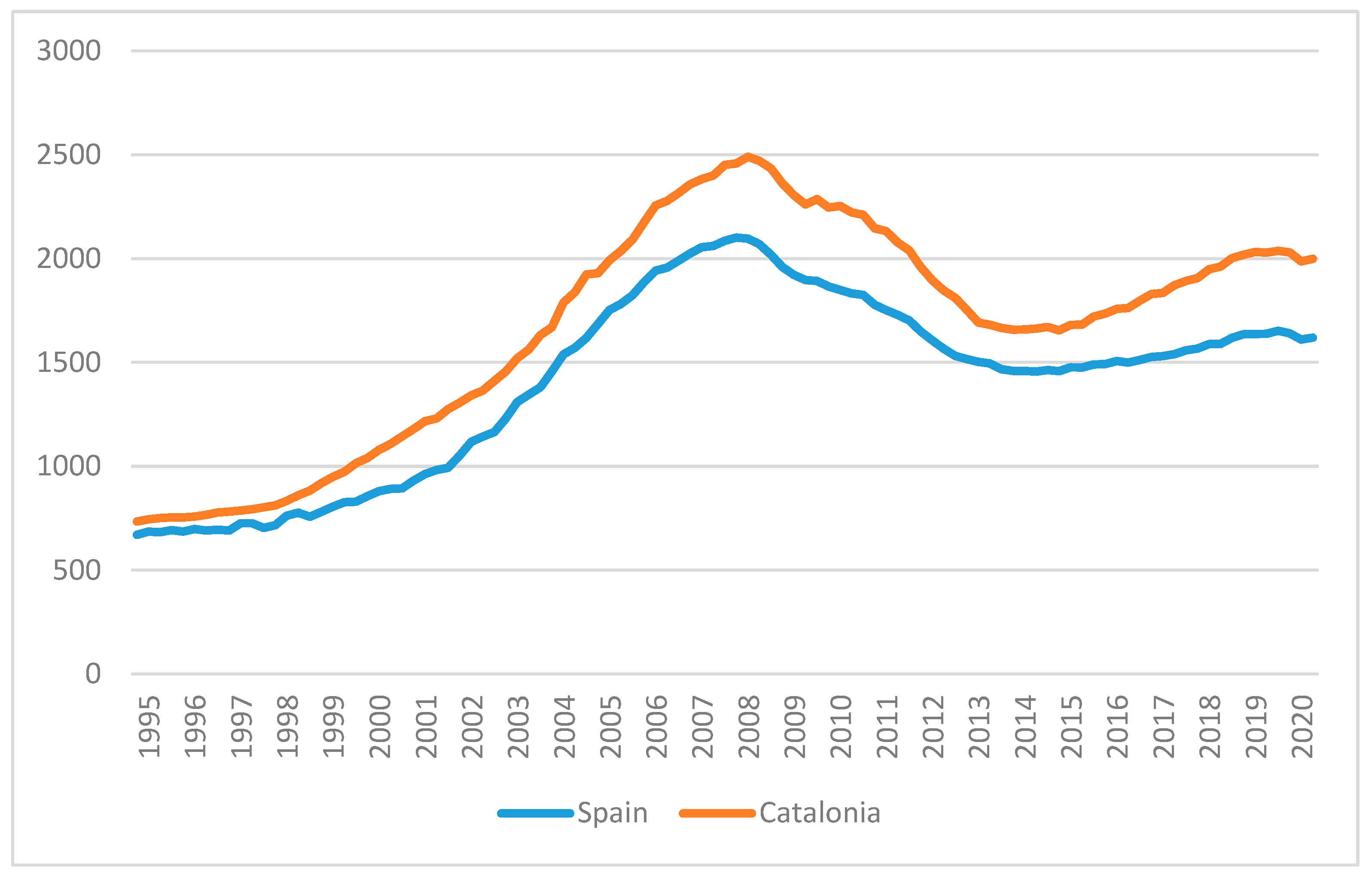73]. Finally, the performance of the Catalan and the Spanish housing market are homogenous. 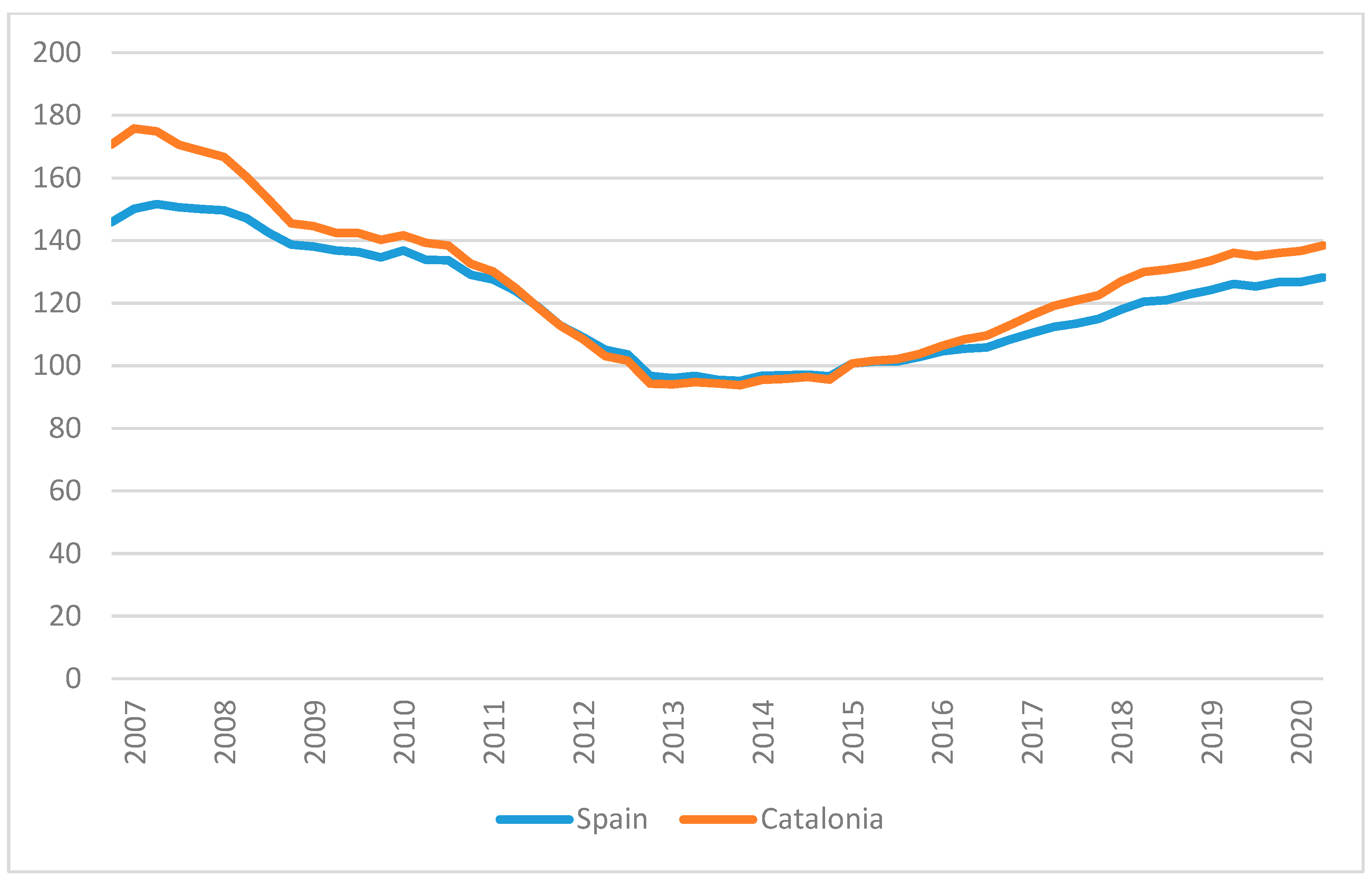For instance, the price per square meter in the free market of dwellings (Figure 1) calculated since 1995 by the Ministry of Transport, Mobility and Urban Agenda (Ministerio de Transportes, Movilidad y Agenda Urbana) [74] shows that in both Catalonia and Spain, the increase of prices extended through to 2008, with a marked growth since the beginning of the century, prices dramatically fell through to 2014 and, thereafter, started a moderate increase. In fact, the correlation of these prices between Catalonia and Spain is significant (<0.01), with a Fisher correlation coefficient of 0.995. Likewise, similar trends are shown in Figure 2 in regard to the Housing Price Index (Índice del Precio de la Vivienda) published by INE [71] since 2007, with a significant (p < 0.01) correlation of 0.986. As such, Catalonia can be considered a representative housing market of Spain.

Overall, the aim of this study was threefold in that it focused on answering the following three questions: (1) Is QR valuation modelling of hedonic prices in the housing market an alternative to ANN? (2) Do housing assessments in the case of Catalonia confirm that ANNs produce better results than SLRs, as it does in other markets? (3) Out of the three analysed models, should all Spanish banks use the same mass appraisal model to assess real estate? In this paper, we present new evidence to compare the performance of QR and SLR hedonic models relative to ANN modelling using the data of properties owned by two banks.

The paper is structured as follows: the methodologies that were used are analysed in Section 2. The datasets used and the analysed variables are described in Section 3. Thereafter, the performance results of the models created are shown and discussed in Section 4. Finally, Section 5 includes the main conclusions and recommendations about the valuation methods to be used by banks and proposals for further research.

2. Methodology

Three methods were used in this study in order to value properties: ANNs, SLRs and QRs.

Neural networks are universal approximators of functions [75,76,77] and are used to adjust functions and also to estimate results. Even though the inception of ANNs can be found in the 1960s [78,79], they became more prevalent at the end of the last century as an alternative to the predominant Boolean logical computation [80].

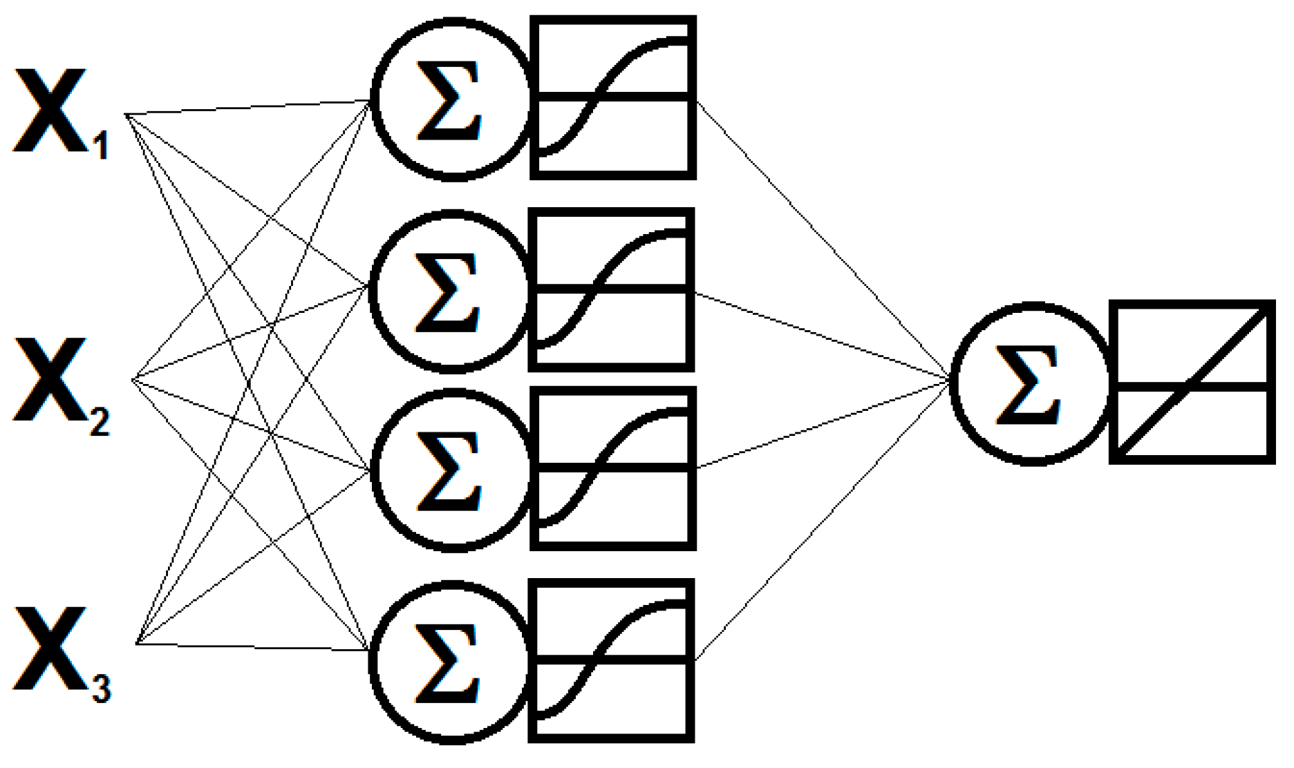
Neural networks are based on an artificial neuron, which processes data in a similar way to a biological neuron named a perceptron [81]. Even though a single neuron cannot undertake a logical process on its own, it is possible for a group of them to do it. This is the reason why neurons are grouped in layers such that they can be used to make logical calculations in networks. A typical neural network has three layers. The first one works as data input. In the second one, which is hidden, data are processed. The third one works as data output. Every single neuron in a layer is connected to every neuron of the following layer via synaptic weights. Hence, when a neuron obtains a result, it is sent to all the neurons in the following layer [82] (see Figure 3).

The most used supervised neural network is known as a multilayer perceptron (MLP) [75,83]. It consists of a three-layer network (input, hidden and output) that uses sigmoid functions as the transference function in the hidden layer.

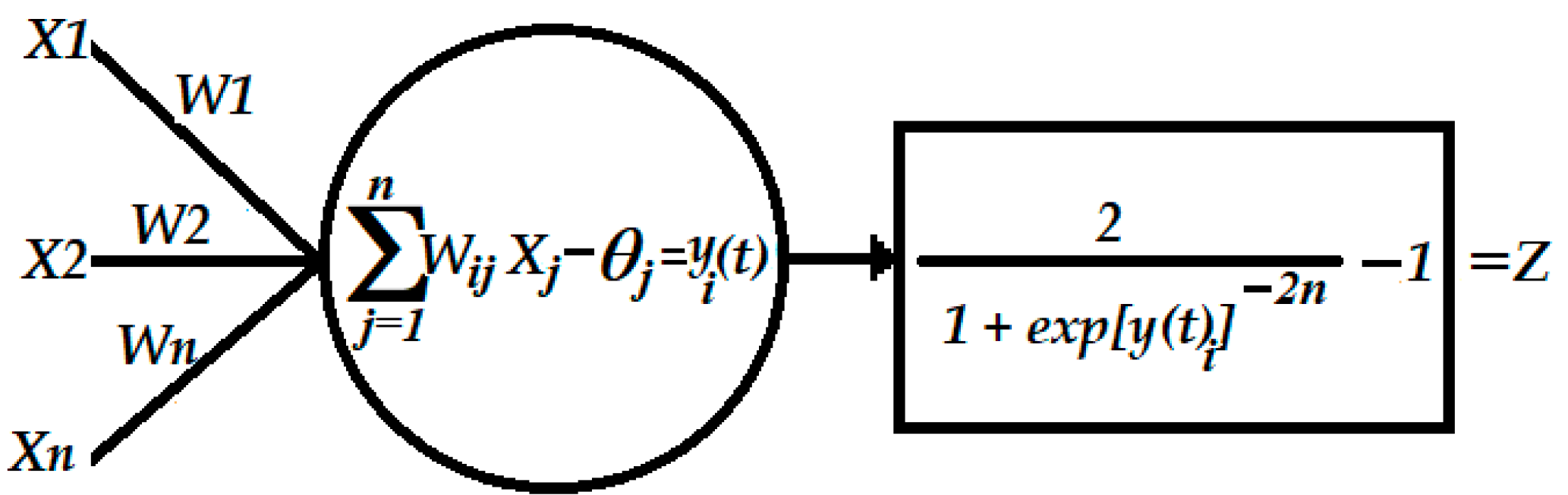
The basis of this model is the artificial neuron (AN). It is a mathematical representation of a biological neuron. A representation of a perceptron is given in Figure 4. The AN receives inputs (X₁, X₂, …, X_N) and these inputs are weighted (W₁, W₂, …, W₃). When the sum-product of the inputs and weights exceeds a threshold (θ_i), the exceeded part is the input of the transfer function. This function is usually a sigmoid (Equation (1)) or tan-sigmoid function (Equation (2)).

$$f\left(x\right)=\frac{1}{1+e^{-x}}$$

(1)

$$f\left(x\right)=\frac{2}{1+e^{-2x}}-1$$

(2)

The result of the transfer function is the output of the perceptron. It can be summarised as follows:

$$Z=\frac{2}{1+e^{-2{{\displaystyle \sum }}_{i=1}^n{x}_i{w}_i-{\theta }_i}}-1.$$

(3)

The key characteristic of an ANN is its capacity to learn. The algorithm used to learn in an MLP is backpropagation (BP), which updates the synaptic weights according to the existing error between the value calculated by the network and the required one [82,84,85].

To find out the nonlinear connections between two groups of data, a neural network needs to be “trained” [86]. This is the reason why the input data, as well as the results that the analyst wants to obtain, are provided to the network. The network that repeatedly uses BP changes the weights (which have a random value at the beginning of the network) until it finds that a group of them that achieve the expected results. Once it has been trained, new data are provided to the network and it is tested to check the goodness of the group of weights. If it is not satisfactory, the weights are readjusted. When the network is tested and its efficiency is optimal, it is ready to work. BP is a generalisation of the Widrow-Hoff law in multilayer networks with non-linear transfer functions. BP allows the artificial neural network to be a universal approximator of functions. Biased networks, such as a sigmoid layer, and a linear output layer can work as approximators of any function with a specific number of discontinuities. BP is a gradient descent algorithm, meaning that the network weights are moved along the negative of the performance function’s gradient. By just implementing the backpropagation learning, we can update the network weights and biases to make the performance function decrease quicker via the negative gradient.

BP is used to estimate the error between the output of an ANN and the goal. The procedure consists of proposing an error or cost function, which measures the network’s performance. This function is determined by the synaptic weights (W). We can obtain the weight upgrade rule by means of the optimization methodology used in the error function. The error function is defined as E(W), which shows the mistake (E) that has been produced by the network. This error is converted into a cost function through the mean quadratic error.

The minimization of the cost function is done by means of a descent down the gradient in the hidden layer and the output layer. The upgrade of the weights is done by deriving the transfer functions.

The steps taken to train an MLP using BP are the following:

• The weights and thresholds (t = 0) are randomly assigned.
• For any pattern (μ) of input data:
  • Execute the network to obtain the output for the μ pattern.
  • Obtain the errors in hidden and output layers.
  • Calculate the increase of weight and threshold for each μ pattern.
• Calculate the total increase in all weights and the threshold for all patterns.
• Upgrade the weights and thresholds.
• Calculate the new error for t = t + 1 and return to step 2 [77].

This process is carried out for every learning set pattern. The upgrade of the weights and thresholds is done after the variation of weights for each pattern. After accumulating all these variations, all the weights are upgraded. This scheme is known as “batch learning”.

The most common mistake made with ANNs is overtraining. The net learns so much that it fits exactly to input patterns. However, the problem is that, perhaps, this overtrained net will not be able to generalise and estimate future patterns. The solution is the early stop. We stop the training when we detect an increase in the total error.

All neural nets are MLP types with three layers: input, hidden and output. Following Demuth et al.’s criterion [87], both the input and hidden layers had the same number of neurons (nodes) as the number of the variables of the model. All the inputs were normalised according to their maximums and minimums in order to be able to train the network. The transfer function was a tan-sigmoid in all nodes in the hidden layer, while the function of the neurons in the output layer was linear. The output layer had only one neuron, which gave us the result of the neural net. We trained the neural nets with a backpropagation algorithm with an early stop to avoid overtraining. The aim was to obtain a better generalisation of the final model. The entire process was done using Matlab. Aside from neural networks, in this study, we estimated hedonic equations using ordinary least squares (OLS) (see [88,89]) and QR (we estimated 10th, 25th, 50th, 75th and 90th quantiles; Appendix A shows the quantile regression model used, which was based on [90]. In order to calculate the price characteristics (including time and location), the following equation was estimated [91]:

$${\mathrm{Price}}_{it}={\beta }_0+{\displaystyle \sum _{k=1}^{k=K}{\beta }_k{X}_{ik}}+{\displaystyle \sum _{l=1}^{l=L}{\alpha }_l{D}_l}+{\displaystyle \sum _{t=1}^{t=T}{\delta }_t{D}_t}+e_{it}$$

(4)

where the aim was to try to explain the price of a dwelling (${\mathrm{Price}}_{it}$) based on its characteristics ($X_{ik}$), the postal code in which it is located ($D_l$) and the year ($D_t$) in order to know the time trend. Finally, ${\beta }_k,{\alpha }_l\mathrm{and}{\delta }_t$ are parameters and $e_{it}$ is the disturbance term, which follows the usual assumptions: the disturbance term is distributed as a normal function and is not correlated, and though it presents heteroskedasticity, the variance of the errors has been estimated in a robust way.

Therefore, this regression model provided estimates of the homogeneous parameters of dwellings, and the hedonic price theory justified its application. In the context of housing, it can be easily appreciated that the valuations that individuals make in relation to the physical characteristics of their dwellings differ according to their prices. Therefore, we aimed to find out the behaviour of the explanatory variables, as well as the price distribution. Consequently, an estimator that allows for heterogeneous responses was required: the estimator stemming from the QR (β_i). Additionally, a median-based (quantile) estimator was also appealing, given that it is less sensitive to outliers than a mean-based estimator. Thus, the bias from unobserved characteristics (i.e., renovation, quality) should be smaller.

In an estimated QR, before the estimation, the target is a parameter that is specified. On the one hand, let e_it be the residual implied by the econometric model (Equation (4)). On the other hand, let q represent the target quantile from the distribution residuals. Thus, the quantile parameter estimates are the coefficients that minimise the following objective function:

$${\displaystyle \sum _{e_{it}>0}2q\left|e_{it}\right|+}{\displaystyle \sum _{e_{it}<0}2(1-q)\left|e_{it}\right|}.$$

(5)

For instance, equal weights are given to positive and negative residuals at the median (q = 0.5). However, at the 90th percentile (q = 0.9), more weight is given to positive residuals. Then, Equation (5) will be minimized at a set of parameter values; where 100q% of the residuals are positive. In this regard, this criterion is classically known as minimum absolute deviations. As a matter of fact, it tends to be used by employing the Koenker and Bassett Jr. [92] algorithm.

As far as the performances of the models were concerned, we used the following:

• Mean squared error (MSE): the mean of the square distance between the target value and the estimated value. It measures the quality of the estimator by measuring the mean squared error of our estimations. The higher this value is, the worse the model is.

$$\mathrm{MSE}\left(y,\widehat{y}\right)=\frac{1}{n}{\displaystyle \sum }_{i=0}^n{\left(y_i-\widehat{y_i}\right)}^2$$

(6)

• Root mean squared error (RMSE): the square root of the MSE, i.e., it is calculated as the square root of the average of the quadratic differences between a variable and its estimation. RMSE is a measure of accuracy. It measures the amount of error between two datasets. To put it another way, it compares an estimated value and a known or observed value. This is one of the most commonly used statistics.

$$\mathrm{RMSE}\left(y,\widehat{y}\right)=\sqrt{\frac{{{\displaystyle \sum }}_{i=1}^n{\left(y_i-\widehat{y_i}\right)}^2}{N}}$$

(7)

• Mean absolute error (MAE): the mean absolute distance between the target value and the estimated value, i.e., the average of the sum of the absolute differences between a variable and its estimation. The same scale as the data being measured is used in MAE. It is known as a scale-dependent measure of accuracy and, thus, it cannot be used to make comparisons between series using different scales.

$$\mathrm{MAE}\left(y,\widehat{y}\right)=\frac{1}{n}{\displaystyle \sum }_{i=0}^n\left|y_i-\widehat{y_i}\right|$$

(8)

• Mean absolute percentage error (MAPE): the mean absolute distance between the target value and the estimated value divided by the target value, i.e., the average sum of the relative difference between a variable and its estimation. It is a measure of the estimation’s accuracy. The mean absolute percentage error is an indicator of the performance of the demand estimation, which measures the size of the absolute error in percentage terms. It is useful even when the volume of demand for the product is not known since it is a relative measure.

$$\mathrm{MAPE}\left(y,\widehat{y}\right)=\frac{1}{n}{\displaystyle \sum }_{i=1}^n\left|\frac{y_i-\widehat{y_i}}{y_i}\right|$$

(9)

• R-squared coefficient (R²): this provides information regarding to what extent the variance of a variable explains the variance of another variable. It is calculated as one minus the proportion between the square error from an estimation of a variable and the square error from the average of the same variable. It provides the measure of the accuracy of replication. The R² is the indicator that allowed us to know how well these results can be estimated. Therefore, R² is the variation percentage of the response variable that explains its relationship with one or more predictor variables. It can be said that, generally, the higher R² is, the better the model fits the data.

$$R^2\left(y,\widehat{y}\right)=1-\frac{{{\displaystyle \sum }}_{i=0}^n{\left(y_i-\widehat{y_i}\right)}^2}{{{\displaystyle \sum }}_{i=0}^n{\left(y_i-\overline{y}\right)}^2}$$

(10)

3. Data

Two datasets consisting exclusively of properties located in Catalonia were analysed. Dataset 1 was provided by a Spanish savings bank that was the result of a merger of three savings banks. The 163,871 properties included in dataset 1 were valued from 1994 to 2010 by independent appraisal companies. Dataset 2 was provided by a former Spanish savings bank that was also the result of a merger of three savings banks. Nevertheless, when the database was provided, the savings bank had been transformed into a commercial bank. The 24,781 properties included in dataset 2 were valued from 2004 to 2013 by independent appraisal companies. As explanatory variables, nine hedonic variables (dwelling characteristics), among which the postal code and year of the observation were included.

Table 1. Definitions of the explanatory variables.

	Variable	Type	Definition
	ln(PriceA)	Quantitative	Natural logarithm of the appraisal price
Hedonic variables	Height	Qualitative	The height of the house ranging from −2 to 19
	Elevator	Dichotomous	Whether the access to the house is by means of an elevator (1 = yes, 0 = no)
	Heating	Dichotomous	Whether the house uses a heating system (1 = yes, 0 = no)
	Pool	Dichotomous	Whether the house or the residents’ association property includes a swimming pool (1 = yes, 0 = no)
	Gardens	Dichotomous	Whether the house or the residents’ association property includes a garden (1 = yes, 0 = no)
	Size	Quantitative	Constructed area of the house in square meters
	Condition	Dichotomous	Physical state of the house (meaning 1 = good, 0 = bad)
	Baths	Quantitative	Number of baths per house
	Rooms	Quantitative	Number of rooms per house
	PC	Qualitative	Postal code
	Year	Quantitative	Year when the house was priced

shows these variables and their definitions in detail, while

Table 2. Descriptive statistics of the quantitative variables.

Variable	Dataset 1		Dataset 2
	Mean	Std. Dev.	Mean	Std. Dev.
ln(PriceA)	12.025	0.683	11.839	0.553
Size	131.025	80.575	85.672	63.464
Baths	1.595	0.703	1.295	0.660
Rooms	3.127	0.855	2.533	1.233
N	163,871		24,781

and

Table 3. Descriptive statistics of the qualitative and dichotomous variables.

Variable	Dataset 1		Dataset 2
	Median	Mode	Median	Mode
Height	2.000	0.000	1.000	0.000
Elevator	0.000	0.000	0.000	0.000
Heating	1.000	1.000	0.000	0.000
Pool	0.000	0.000	0.000	0.000
Gardens	0.000	0.000	0.000	0.000
Condition	1.000	1.000	0.000	0.000
N	163,871		24,781

show the descriptive statistics for quantitative, as well as qualitative and dichotomous variables, respectively.

The combined number of properties analysed was 188,652, which represented 4.88% of the total number of the Catalan housing stock according to the official statistics published by INE [71]. On the other hand, the number of postal codes analysed amounted to 632 in dataset 1 and 607 in dataset 2; this meant that the properties analysed were not concentrated in a specific area, on the contrary, they are a good sample of Catalan housing (Catalonia comprises 1146 postal codes). Furthermore, the years analysed—1994 to 2013—covered both the rise and fall of real estate prices in Catalonia. Finally, according to the official statistics published by the Spanish Government by means of Ministry of Transport, Mobility and Urban Agenda (Ministerio de Transportes, Movilidad y Agenda Urbana) [93], the number of housing transactions from 2004 to 2013 was 890,554. On the other hand, the number of properties analysed in which prices corresponded to these years totalled 122,179. Hence, this amounted to 13.72% of the whole Catalan housing market for the decade studied.

4. Results and Discussion

Twelve models were created per dataset using the natural logarithm of the appraisal as the variable to be explained: four ANNs), four SLRs and four QRs. We have used some quasi-Newton algorithms (such as the Broyden-Fletcher-Goldfarb-Shanno (BFGS) method [87] and one-step secant), with the Levenberg-Marquardt algorithm being the one that performed better. Therefore, we have used supervised ANNs, with backpropagation (Levenberg-Marquardt) learning algorithms and an early stop.

Table A1. Architecture of the developed ANN model.

Property	Structure
Number of hidden neurons	The same number as the input layer
Transfer function in the hidden layer	Tan-sigmoid
Transfer function in the neuron of output layer	Linear
Type of learning rule	Backpropagation with the Levenberg–Marquardt algorithm
Control of overlearning	Early stop

in Appendix B shows the architecture of the developed ANN model. The models differ because different explanatory variables were used to create them: 1 means that only hedonic variables were used; 2 means that hedonic variables and postal code were used; 3 means that hedonic variables, postal code and year were used, therefore, all the explanatory variables were used; 4 means that all the explanatory variables were used and that we also controlled for postal code and year by means of transforming them into dummy variables.

The performances of these models are presented in

Table 4. Comparison of the performances of artificial neural networks (ANNs), semi-log regressions (SLRs) and quantile regressions (QRs) for dataset 1.

Performance Measure	ANN 1	ANN 2	ANN 3	ANN 4	SLR 1	SLR 2	SLR 3	SLR 4	QR 1	QR 2	QR 3	QR 4
MSE	0.2933	0.2750	0.1107	0.1096	0.3141	0.1622	0.1162	0.1162	0.8533	0.8332	0.3120	0.2994
RMSE	0.5416	0.5244	0.3326	0.3311	0.5604	0.4028	0.3409	0.3409	0.9237	0.9128	0.5586	0.5472
MAE	0.4273	0.4128	0.2269	0.2278	0.4458	0.3982	0.1983	0.1969	0.7911	0.7808	0.4763	0.4642
MAPE	0.0361	0.0349	0.0192	0.0193	0.0371	0.0328	0.0188	0.0186	0.0772	0.0667	0.0432	0.0398
R2	0.3712	0.4105	0.7628	0.7651	0.3267	0.4680	0.8180	0.8200	0.2358	0.2452	0.4084	0.4124

for dataset 1 and in

Table 5. Comparison of the performance of the ANNs, SLRs and QRs for dataset 2.

Performance Measure	ANN 1	ANN 2	ANN 3	ANN 4	SLR 1	SLR 2	SLR 3	SLR 4	QR 1	QR 2	QR 3	QR 4
MSE	0.2088	0.1706	0.1238	0.1273	0.2294	0.1190	0.0866	0.0853	0.6363	0.5491	0.4900	0.4742
RMSE	0.4569	0.4131	0.3519	0.3568	0.4790	0.3450	0.2943	0.2920	0.7977	0.7410	0.7000	0.6886
MAE	0.3571	0.3196	0.2595	0.2633	0.3730	0.2711	0.2172	0.2159	0.6851	0.6311	0.5022	0.4979
MAPE	0.0305	0.0272	0.0221	0.0224	0.0321	0.0218	0.0181	0.0175	0.0580	0.0550	0.0455	0.0445
R2	0.3171	0.4419	0.5951	0.5835	0.2492	0.5900	0.7081	0.7150	0.2129	0.2470	0.5351	0.5360

for dataset 2 in terms of MSE, RMSE, MAE, MAPE and R². We tested the models by means of a dataset of properties with transaction prices instead of appraisal prices, obtaining similar results (see

Table A2. Comparison of the performance of the ANNs, SLRs and QRs for the dataset with transaction prices.

Performance Measure	ANN 1	ANN 2	ANN 3	ANN 4	SLR 1	SLR 2	SLR 3	SLR 4	QR 1	QR 2	QR 3	QR 4
MSE	0.1666	0.1334	0.1056	0.1675	0.2221	0.1416	0.0671	0.0663	0.5646	0.4756	0.4170	0.4072
RMSE	0.4082	0.3652	0.3249	0.4092	0.4345	0.3469	0.2389	0.2374	0.6927	0.6358	0.5954	0.5883
MAE	0.3187	0.2819	0.2436	0.3163	0.3391	0.2758	0.1903	0.1721	0.5769	0.5436	0.4984	0.4875
MAPE	0.0268	0.0237	0.0204	0.0274	0.0297	0.0199	0.0163	0.0148	0.0503	0.0480	0.0430	0.0423
R2	0.3072	0.4449	0.5609	0.4934	0.1783	0.4161	0.6436	0.6562	0.1429	0.1946	0.2269	0.2278

).

The results suggest that the ANNs and SLRs were better tools than QRs for modelling housing prices in Catalonia. In fact, the results in terms of all common performance measures for all the models and datasets were better for the ANNs and SLRs than for the QRs. On the one hand, the ANNs were better than SLRs when only hedonic variables were used. On the other hand, when more variables were used, SLRs obtained better results using dataset 2, whereas the performance results were not conclusive for dataset 1 when more variables were used, independent of whether the year was considered a dummy variable. Finally, all the models obtained better results when more variables were included and the use of time as a dummy variable slightly enhanced the results obtained for the SLRs and QRs for all datasets. The improvement of the results from ANN1 to ANN2 was studied by McGreal et al. [48], who asserted that better results were obtained by neural networks when the postal code was used as a delimiter. This makes sense because location effects are crucial when estimating real estate prices. Following the same line of reasoning, the real estate market is dynamic and time-fixed effects are also crucial in their estimation. On the contrary, the use of time as a dummy variable does not improve the models obtained by means of ANN. In other words, when using an ANN, transforming a quantitative variable into dummies will generate the same results. This was confirmed by Peterson and Flanagan [45], who stated that since the parametric estimation in an ANN does not depend on the range of the regressive matrix, ANNs are better than the models that need to use large sets of dummies. In fact, the performance results for ANN models were worse for dataset 2 and inconclusive for dataset 1 when time was used as a dummy variable in comparison to when it was considered as a quantitative one.

The results suggest that the ANN models improved when the analysed dataset was larger. In fact, when the smallest dataset was used, the SLR results were better than the ones obtained by the ANNs. Therefore, we agree with Worzala et al. [49], who compared ANNs with traditional multiple regression models and no evidence was found demonstrating that ANNs are superior for valuation analysis. Nevertheless, our results demonstrate that they are not worse, except regarding the R² coefficient, where only similar results were obtained using SLR methodology when the largest dataset is used. This is confirmed by Nghiep and Cripps [50], who determined that ANNs obtain results that are similar to those obtained using regression models when a large sample is used.

5. Conclusions

This paper presents new evidence to compare the performances of QR and SLR hedonic models relative to ANNs using data of properties that belonged to two banks. The aim of this study was threefold:

First, this study aimed to cover the literature gap in regard to the comparison of QRs and ANNs for assessing hedonic prices in housing, with this being the first article to include this comparison. The results suggest that QRs are worse tools than ANNs when modelling housing prices in Catalonia. Therefore, QR valuation modelling cannot be considered as an alternative to ANNs given that its performance was worse for all datasets, regardless of the number of variables used.

Second, when using all the variables, the SLRs performed better than the ANNs with the smallest dataset, whereas the results were not conclusive in regard to the largest dataset. Therefore, in the specific case of Catalonia, we cannot confirm the fact observed in other markets that suggest that ANNs perform better than SLR when assessing real estate. Third, out of the three models analysed and according to the results obtained, Spanish banks should use a model for housing mass appraisals that matches their size. Small and medium banks (mainly cooperatives and savings banks) should use SLRs rather than ANNs given that SLRs are better when the dataset was smaller. On the other hand, large banks (mainly commercial banks) can use either SLRs or ANNs given that their performance was similar for larger datasets. Finding out the optimal way to value properties registered in banks’ balance sheets has been one of the greatest challenges that the banking industry has faced in recent years. An optimal valuation offers two advantages: first, the real financial situation of the bank is established; second, if the property is valued according to the market, it can be sold more quickly and the revenues obtained will be maximised. Overall, given that this study was carried out with data obtained previous to the recent legislation that has limited rental prices in Catalonia (Law 11/2020, issued on 18 September 2020) and that the Catalan real estate market is representative of the Spanish market, the conclusions can be generalised to the whole country of Spain.

With regard to the limitations of this paper, we must recognise that the main one has to do with the fact that datasets used included prices through to 2013. It would be very useful to obtain more recent and similar databases. Nonetheless, it is highly unlikely that the authors may obtain such a database in the future since it is usually not available to researchers due to opacity of information given by banks. Nevertheless, the conclusions obtained by means of this study can be considered important because the lifespan of the data analysed ranged from 1994 to 2013. Therefore, boom and recession years in the housing industry were included due to the fact that this time horizon encompassed the rise and fall of the Spanish real estate bubble.

Future lines of research could include the analysis of more recent large databases, in the event of them becoming available. Additionally, by means of a simulation exercise, future studies could analyse the extent to which banks would have benefited—by means of an increase of revenues, capital gains generation and the reversal of impairment losses—from having used these models.