Mexican Axolotl Optimization: A Novel Bioinspired Heuristic

Abstract

When facing certain problems in science, engineering or technology, it is not enough to find a solution, but it is essential to seek and find the best possible solution through optimization. In many cases the exact optimization procedures are not applicable due to the great computational complexity of the problems. As an alternative to exact optimization, there are approximate optimization algorithms, whose purpose is to reduce computational complexity by pruning some areas of the problem search space. To achieve this, researchers have been inspired by nature, because animals and plants tend to optimize many of their life processes. The purpose of this research is to design a novel bioinspired algorithm for numeric optimization: the Mexican Axolotl Optimization algorithm. The effectiveness of our proposal was compared against nine optimization algorithms (artificial bee colony, cuckoo search, dragonfly algorithm, differential evolution, firefly algorithm, fitness dependent optimizer, whale optimization algorithm, monarch butterfly optimization, and slime mould algorithm) when applied over four sets of benchmark functions (unimodal, multimodal, composite and competition functions). The statistical analysis shows the ability of Mexican Axolotl Optimization algorithm of obtained very good optimization results in all experiments, except for composite functions, where the Mexican Axolotl Optimization algorithm exhibits an average performance.

1. Introduction

Sometimes when researchers are faced with certain problems in science, engineering, or technology, it is not enough to find a solution, but it is essential to find the best possible solution, or in other words, to optimize. Optimization refers to the process by which one tries to find the best possible solution for a given problem, usually in a limited time. Colloquially it has been used imprecisely as a meaning of “doing better”. Multivariate function optimization (minimization or maximization) is the process of searching for variables x₁, x₂, x₃, …, x_n that either minimize or maximize some function f(x₁, x₂, x₃, …, x_n) [1].

Most optimization problems are described by mathematical functions with some specific characteristics, which make them impossible to solve by traditional analytical ways. To deal with such functions, several exact procedures have been proposed. However, in some cases, the computational complexity of the exact procedures makes them inapplicable to certain function optimization problems, as in the well-known case of the Traveling Salesman Problem [2].

As an alternative to exact optimization, approximate optimization algorithms aim at reducing the computational complexity of the search by pruning some areas of the search space of the problem. To do so, researchers have often found inspiration in nature, due to animals and plants showing interesting behaviors for solving complex problems. For example, ants are able to find a minimum-length path from their nest to the available food sources [3].

Perhaps the first bioinspired algorithms for numerical optimization are Genetic Algorithms, developed by John Holland in the 1970s [4]. Since then, several optimization algorithms based on evolution had been proposed, such as Genetic Programming [5] and Differential Evolution [6]. In this context, numerous bioinspired algorithms have been proposed [7], with several applications in industry [8], business [9], medicine [10], education [11], and other fields.

The purpose of this research is to obtain inspiration from nature, and to design a novel bioinspired algorithm for numeric optimization. We believe that nature is filled with incredible flora and fauna, showing amazing behaviors that can be useful for the design of intelligent algorithms, leading to solving problems the of industry, business, and others by the optimization of mathematical functions describing the related phenomena.

The main contribution of this paper is introducing a novel bioinspired algorithm for numerical optimization: the Mexican Axolotl Optimization (MAO) algorithm. MAO is compared against several existing bioinspired algorithms over four sets of benchmark functions, comprising unimodal, multimodal, composite and competition functions. The statistical analysis shows the ability of MAO to obtain good optimization results, being significantly better than other state-of-the-art bioinspired optimization algorithms.

The paper is structured as follows: Section 2 reviews some of the developments made in bioinspired optimization, Section 3 details the proposed MAO algorithm, and Section 4 shows the numerical experiments made. The paper ends with the Conclusions, References and Appendices.

2. Related Works on Bioinspired Optimization

Numerous bioinspired algorithms had been proposed for numerical optimization. In this section we briefly explain the functioning of some of the most important ones.

Differential Evolution (DE) [6] is perhaps one of the most used evolution-based bioinspired optimization algorithm to date, with numerous applications [12]. DE creates a population of solutions, and then evolves such a population by two operators: mutation and recombination. The initial population of solutions is chosen at random and must cover the entire parameter space. The mutation operator within the DE is a process by which, from an existing population of solutions, new individuals are produced for subsequent generations. To do so, for each individual, three different solutions are selected, and a mutated solution is obtained by adding the weighted difference between two population solutions to a third solution. The weighing is performed by using a constant $\mathrm{F}$. Usually, $\mathrm{F}\in \left[0.1, 1.0\right]$.

Once the mutation process has been carried out, a recombination operation is conducted, which has the primary objective of increasing the diversity of the individuals of the next generation. In this operation, the components of the solution are recombined in order to generate an intermediate individual. This recombination operation recombines the elements of both the target individual and the mutated individual, following a crossing constant $\mathrm{CR}\in \left[0,1\right]$, which will determine if the component to be preserved will come from the mutated individual or the target individual [12].

The selection operation is the last that is carried out to determine the new individuals that will be part of the next generation within the evolution process. In this operation it is decided whether an intermediate individual will be part of the next generation, or not. To determine this, the intermediate individual is compared to the target individual. If the intermediate individual generated during this process has a better objective function value than the target individual of the current generation, then the new individual of the next generation will be equal to the intermediate individual and the target individual will be replaced, otherwise the individual goal is preserved for the next generation [6].

In nature, animals search for food randomly or almost randomly. Generally, an animal’s feeding path is effectively a random walk because the next move is based on both the current location/state and the probability of transition to the next location [13]. Most of the existing bioinspired optimization algorithms are based on the behavior of animals [14]. In the following, we review some of them.

The Cuckoo Search (CS) algorithm was inspired by the obligate breeding parasitism of some species of cuckoos by laying their eggs in the nests of host birds [15,16]. Some cuckoos have evolved in such a way that female parasitic cuckoos can mimic the colors and patterns of the eggs of a few chosen host species. This reduces the probability that the eggs will be abandoned and, therefore, increases their productivity.

Most of the host birds came into direct conflict with the intruding cuckoos. In this case, if the host birds discover that the eggs are not theirs, they will throw them away or simply abandon their nests and build new ones elsewhere. Parasitic cuckoos often choose a nest where the host bird simply lays its own eggs. In general, cuckoo eggs hatch slightly earlier than the host’s eggs. Once the first cuckoo chick hatches, its first instinctive action is to dislodge the eggs from the host by blindly propelling the eggs out of the nest. Additionally, studies show that a cuckoo chick can mimic the call of the host chicks to access more feeding opportunities. The CS models such playback behavior and can therefore be applied to various optimization problems. Yang and Deb found that CS performance can be improved by using Levy Flights rather than a simple random walk [15,16].

The Firefly algorithm (FA), which was first developed by Yang [17,18] was based on the blink patterns and behavior of fireflies. In essence, FA uses the following three idealized rules:

• Fireflies are unisexual, so a firefly will be attracted to other fireflies regardless of their gender.
• The attractiveness is proportional to the brightness and both diminish as your distance increases. Therefore, for two flashing fireflies, the less bright will move to the brighter. If there is no one brighter than a particular firefly, it will move randomly.
• The brightness of a firefly is determined by the landscape of the objective feature.

The movement of a firefly $i$ is attracted to another firefly j, which is more attractive (brighter).

FA uses two embedded cycles to update the position of the individuals in the swarms, and has obtained very good results in optimization problems [19].

The Dragonfly algorithm (DA) is an optimization procedure based on the behavior of dragonflies [20]. It starts the optimization process by creating a set of random solutions for a given optimization problem. In fact, the position and pitch vectors of dragonflies are initialized by random values defined within the lower and upper limits of the variables. At each iteration, the position and step of each dragonfly is updated. To update the position, the neighborhood of each dragonfly is chosen by calculating the Euclidean distance between all the dragonflies and selecting N of them.

The position update process continues iteratively until the completion criterion is met. DA algorithm considers several aspects such as separation, alignment, cohesion, attraction, distraction, and random walk, which makes it suitable for optimization, and obtained good results [21]. In addition, DA models concepts of static and dynamic swarms.

The Fitness Dependent Optimizer (FDO) [22] bases its operation on the reproduction process of swarms of bees. Each scout bee searching for new hives is considered to converge towards the optimum. The algorithm begins by randomly initializing a population of artificial explorers in the search space. The solutions are hives discovered for the first time and are represented by the positions of the scout bees. The best solutions found replace the ones that were previously the best. FDO was found to perform better than other optimization algorithms [22], such as PSO [23] and Genetic Algorithms [4].

Another recently introduced algorithm is the Monarch Butterfly Optimization (MBO) [24]. This method models the migration of the monarch butterflies, endemic to North America. Such insects travel from Mexico to Canada on a yearly basis. In addition, last year saw the introduction of the Slime Mould Algorithm (SMA), based on the oscillation mode of slime mould in nature. This propagative organism seeks for food, and has an oscillatory behavior [25].

Despite the numerous proposals in the field of bioinspired algorithms [26,27], there is plenty of room for new proposals, due to the fact that nature is rich, and every day we can find inspiration in fauna and flora to obtain better solutions for optimization problems. In the next section, we introduce a novel algorithm based on a one-of-a-kind creature native to Mexico: the axolotl.

3. Mexican Axolotl Variable Optimization

This section briefly explains the life of the axolotl, a very interesting creature native to Mexico, as well as the proposed bioinspired optimization procedure.

3.1. The Axolotl in Nature

The Mexican Axolotl (Ambystoma mexicanum) is endemic to the Valley of Mexico. Its habitat is lakes or shallow water channels with a lot of aquatic vegetation. It is a completely aquatic species. Its diet is very varied and in free life it includes small fish, fry, and prairie fish. In captivity, they are commonly fed tubifex worms, earthworms, worms, and small pieces of raw turkey, chicken, or beef [28].

The axolotl has been in the lives of Mexicans since the time of the Aztecs. According to Aztec mythology, the axolotl (from Nahuatl: atl “water” and xolotl “monster”; water monster), is related to the god Xólotl, Quetzalcoatl’s brother [29]. It has also appeared in contemporary literature: in the story Axolotl by Julio Cortázar (in his End of the Game compendium [30]), and in Frank Herbert’s Dune [31].

In science, the axolotl is known for its extraordinary ability to regenerate amputated limbs and other organs and tissues of the body. It has been observed, for example, that if these animals lose a limb, they are able to regenerate it in a matter of weeks, with all their bones, muscles, and nerves in the appropriate places [32]. Even more fascinating, the researchers say, is the axolotl’s ability to repair its spinal cord when it is injured and make it function as if it had not been damaged. It can also repair other tissues—such as the retinal tissues—and heal wounds without leaving scars. They can also easily accept transplants from other individuals, including the eyes and parts of the brain, restoring their full functionality [33].

This amphibian, which is in danger of extinction in its natural habitat, has also attracted the interest of researchers because of the relative ease with which it can reproduce, and the absence of age-related diseases among its populations [34]. This interesting animal has been cultivated in the laboratory since 1864, and it is used to investigate phenomena such as nuclear reprogramming, the embryology of germ-cell induction, retinal neuron processing and regeneration [35]. An attractive characteristic of axolotls for research is the large size and ease of manipulation of the embryos, which allow to see the complete development of a vertebrate in the egg.

The axolotl measures about 15 cm in total length, with it being rare the specimens that measure more than 30 cm. The axolotl has the appearance of a giant tadpole with legs and a tail. It is characterized by having three pairs of gills, which come out from the base of its head and go backwards, small eyes, smooth skin and legs whose fingers are thin and pointed, but which do not develop nails.

The color of the axolotl is highly variable: in the wild, most are dark brown with a black back, a lighter belly, and faint and not very visible dark spots on the flanks and back. However, they can also present different coloration patterns, especially in captivity: gray, brown, brownish-green, orange and even white with black eyes, golden albino, white albino or almost black [28]. Axolotls also have some limited ability to alter their color to provide better camouflage by changing the relative size and thickness of their melanophores [36].

Axolotls have males and females, and the axolotl reaches sexual maturity at a year of life. At this age it is easy to recognize the sex of the animals; the males are thinner and have large glands around the cloaca. The females tend to have shorter and wider heads, as well as being a bit fatter [28].

The breeding season depends on the hemisphere where they are found; in the northern one it is from February to April, and in the southern one it occurs from August to November. However, clumps can occur in midsummer and in winter. A water temperature of twelve to sixteen degrees centigrade is the most suitable for breeding [37].

Sexual activity as well as egg laying takes place at night. Fertilization is internal; the male places spermatophores (tiny whitish cones that contain the sperm at their tip) on the substrate, or some rock and the female collects them with the cloaca to deposit them in her spermatheca. The next night the laying begins, which can last until the early hours of the day. The female deposits the eggs in groups of four to ten on the plants or trunks. These eggs are provided with a capsule that protects the embryo from infections; without it they inevitably die. They deposit the eggs in different places to guarantee the survival of at least some of them in the event of a predator [28].

Spawning can range from fifty to fifteen hundred eggs; said amplitude of laying depends on the age and sanitary conditions of the female. At 21 h after being fertilized, it is already a blastula, having a smooth surface. When it is three days old, the embryo has an elongated shape. The neural folds are outlined, beginning to rise above the head area. Between three and four days, in the embryo the neural folds at the level of the spinal area fuse. The optic vesicles are developing. A small swelling delimits the future region where the gills will be located. A depression appears in the ectoderm, which will become the primordium of the ear. When 10 days have elapsed, the gills are elongated and already have four pairs of filaments. The mouth is more clearly marked, and the buds already protrude from the limbs [28].

On day 12, the hatching process begins, where the larva makes convulsive movements, thus shedding the layer of gelatin that covered it. The young are considered larvae from hatching to four months. They only have a head, gills, and a body. The limbs will develop later [37].

In their first hours of life, the larvae of the axolotl feed on some of the remains of the yolk, but very soon they will need microalgae, such as spirulina, to feed themselves and continue to develop. When the axolotl is between for and 12 months old it is considered a youngster, generally it already measures about five centimeters. From 13 months the stage begins where it can reproduce, since it is sexually mature [38].

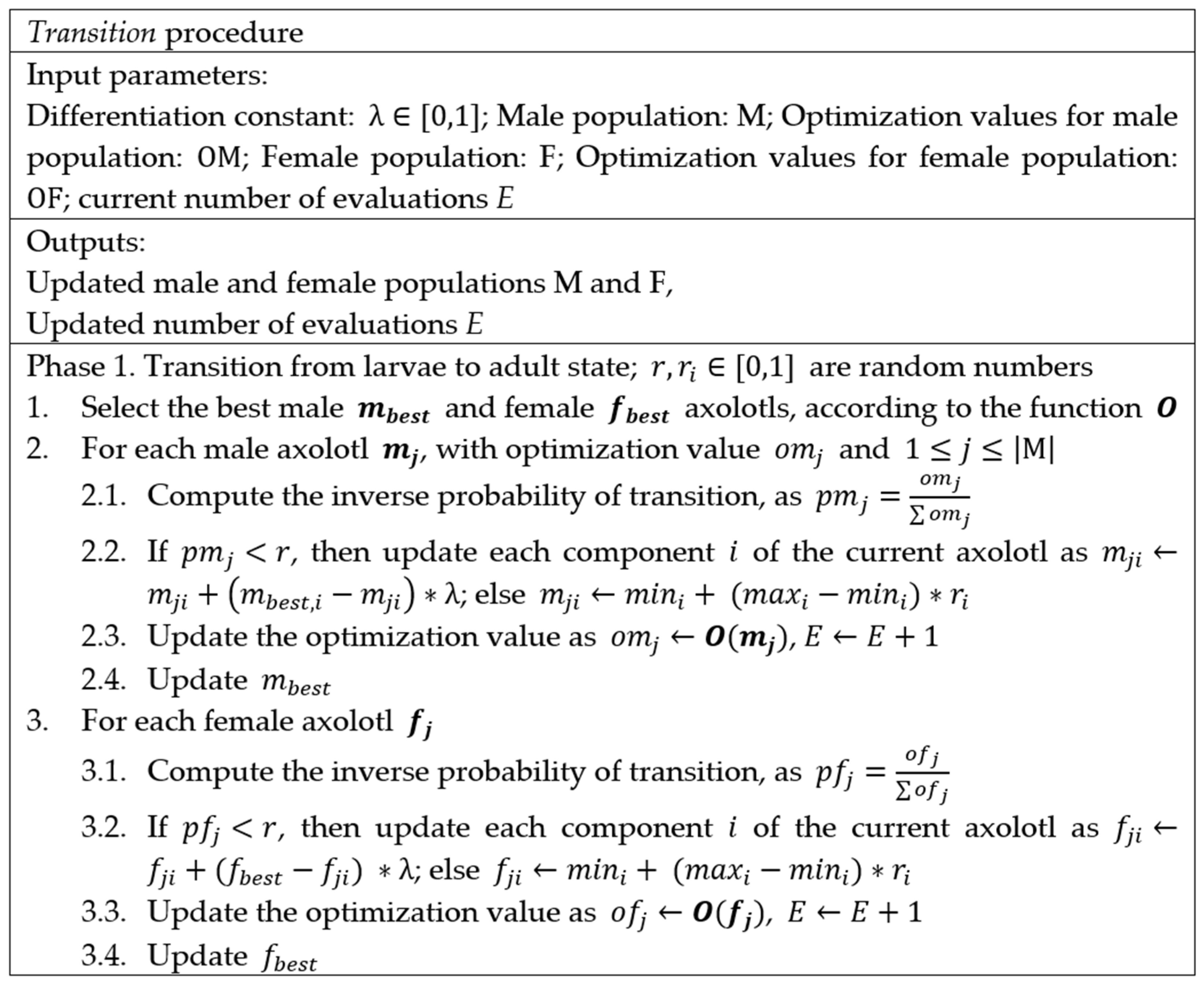
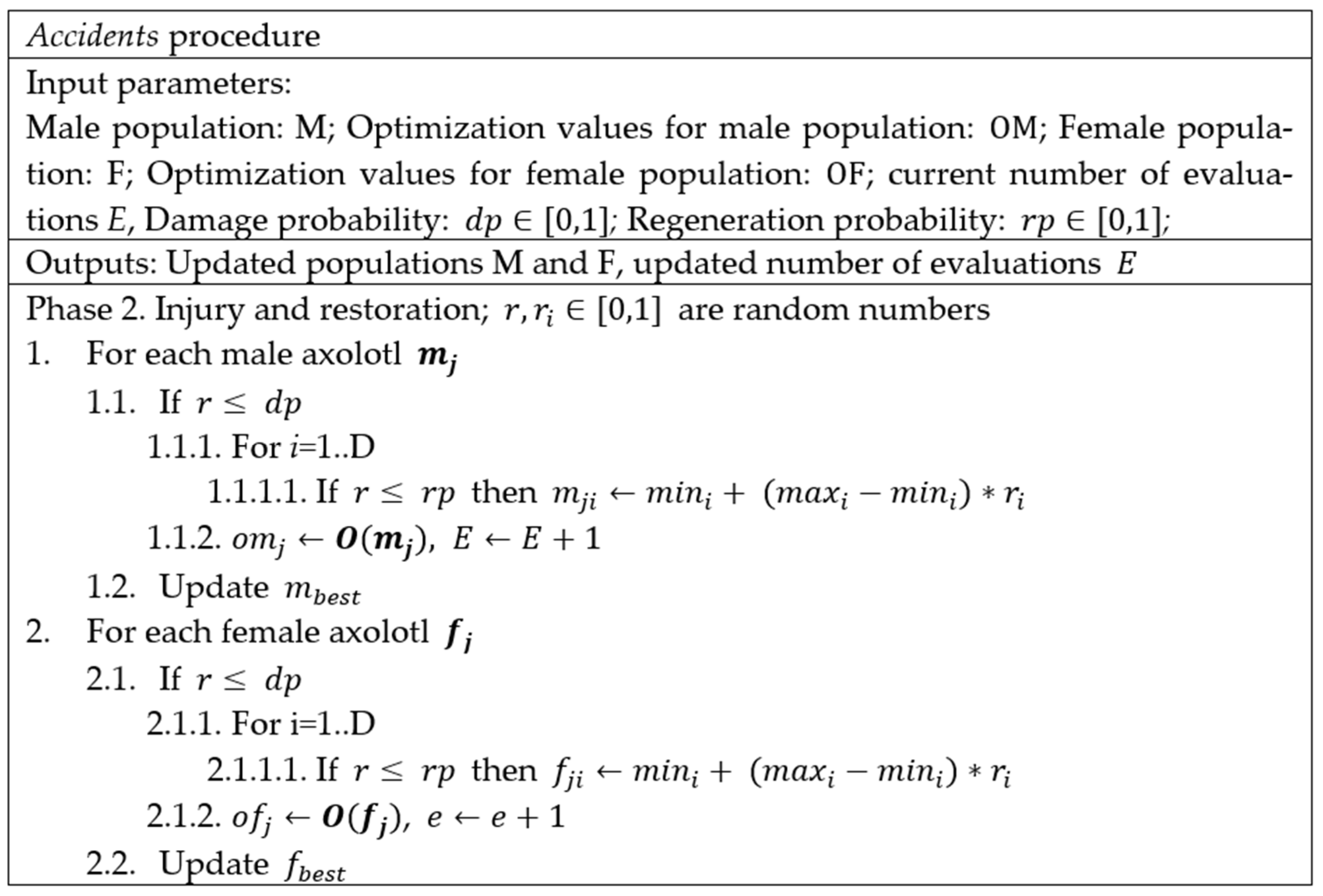
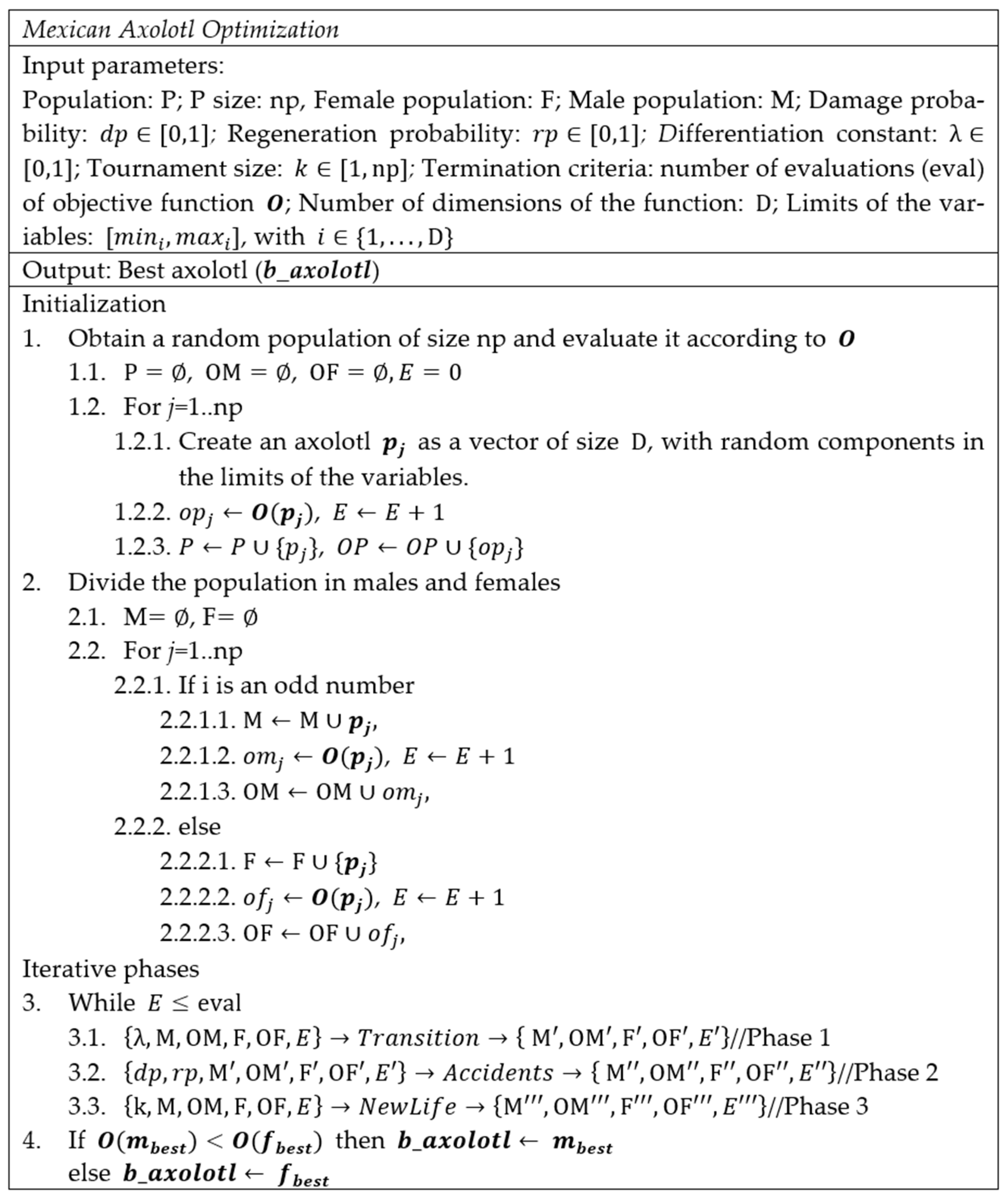
3.2. The Artificial Axolotl

The proposed Mexican Axolotl Optimization (MAO) algorithm inspired by the life of the axolotl is explained in this section. We were inspired by the birth, breeding, and restoration of the tissues of the axolotls, as well as the way they live in the aquatic environment. As axolotls are sexed creatures, our population is divided into males and females. We also consider the ability of axolotls to alter their color, and we consider they alter their body parts’ color to camouflage themselves and avoid predators.

Let us assume that we have a numeric optimization problem, defined by a function $\mathit{O}$ whose arguments are vectors of dimension D, such that each dimension $d_i$ is bounded by $\left[mi{n}_i, ma{x}_i\right]$. We also have a set of solutions (axolotls) of size $\mathrm{np}$, conforming the population $P=\left\{{\mathit{S}}_{\mathbf{1}},\dots ,{\mathit{S}}_{\mathit{n}\mathit{p}}\right\}$, and each solution (axolotl) ${\mathit{S}}_{\mathit{j}}\in P$, $1\le j\le \mathrm{np}$, is represented as a vector of form ${\mathit{S}}_{\mathit{j}}=\left[s_{j1},\dots ,s_{j\mathrm{D}}\right]$, with $mi{n}_i\le s_{ji}\le ma{x}_i$, such that $\mathit{O}\left({\mathit{S}}_{\mathit{j}}\right)\in ℝ$. In the following, we assume that we want to find the minimum value of the function $\mathit{O}$.

The proposed MAO algorithm operates in four iterative stages, defined by the TIRA acronym: Transition from larvae to adult state, Injury and restoration, Reproduction and Assortment.

First, the initial population of axolotls is initialized randomly. Then, each individual is assigned as male or female, due to axolotls developing according to their sex, and two subpopulations are obtained. Then, the Transition from larvae to adult begins. Male individuals will transition in water, from larvae to adult, by adjusting their body parts’ color towards the male who is best adapted to the environment (Figure 1).

We assume that best adapted individuals have better camouflage, and the other individuals will change their color accordingly. However, the ability of the axolotls to change color is limited, and we do not want every individual to be able to fully adapt towards the best, which is why we introduce an inverse probability of transition. According to such probability, an axolotl will be selected to camouflage towards the best.

Let $m_{best}$ be the best adapted male (the one with best value of the objective function $\mathit{O}$), and $\mathsf{\lambda }$ be a transition parameter in [0, 1] for the male axolotl ${\mathit{m}}_{\mathit{j}}$, which will change its body parts’ color as in Equation (1).

$$m_{ji}\leftarrow m_{ji}+\left(m_{best,i}-m_{ji}\right)\ast \mathsf{\lambda }$$

(1)

Similarly, female axolotls change their bodies from larvae to adults towards the female with best adaptation, using Equation (2), where $f_{best}$ is the best female and $f_{\mathrm{j}}$ is the current female axolotl.

$$f_{ji}\leftarrow f_{ji}+\left(f_{best,i}-f_{ji}\right)\ast \mathsf{\lambda }$$

(2)

However, and according to the inverse probability of transition, dummy individuals unable to camouflage themselves towards the best, and having their own colors are selected. To do so, if a random number $r\in \left[0,1\right]$ is lower than the inverse probability of transition, the corresponding individual is selected. For a minimization problem, for a male axolotl ${\mathit{m}}_{\mathit{j}}$, with optimization value $o{m}_j$ the inverse probability of transition is computed as in Equation (3); for female axolotl ${\mathit{f}}_{\mathit{j}}$, with optimization value $o{f}_j$ we use Equation (4). The worst individuals will have greater chances of random transition.

$$p{m}_j=\frac{o{m}_j}{{\sum }^{ }o{m}_j}$$

(3)

$$p{f}_j=\frac{o{f}_j}{{\sum }^{ }o{f}_j}$$

(4)

Those individuals will transition their i-th body parts randomly (considering each body part as a function dimension), as in Equations (5) and (6), where $r_i\in \left[0,1\right]$ is a random number chosen for each i-th body part. The individuals with random transition will be selected according to the value of the optimization function.

$$m_{ji}\leftarrow mi{n}_i+\left(ma{x}_i-mi{n}_i\right)\ast r_i$$

(5)

$$f_{ji}\leftarrow mi{n}_i+\left(ma{x}_i-mi{n}_i\right)\ast r_i$$

(6)

In moving across the water, axolotls can suffer accidents and be hurt. This process is considered in the Injury and restoration phase. For each axolotl $S_i$ in the population (either male or female), if a probability of damage (dp) is fulfilled, the axolotls will lose some part or parts of its body. In the process, using the regeneration probability (rp) per bit, the axolotl will lose the j-th body part (bit), and will replace it as ${p_{ji}}^{\prime }\leftarrow mi{n}_i+\left(ma{x}_i-mi{n}_i\right)\ast r_i$, where $0\le r_i\le 1$ is randomly chosen for each body part.

The pseudocode of the Injury and Restoration phase of the Mexican Axolotl optimization algorithm is provided in Figure 2. Then, the Reproduction of the population begins. The pseudocode of the Reproduction and Assorting phase is given in Figure 3. For each female axolotl in the population, a male is selected from which offspring will be obtained. To do so, we use tournament selection.

After that, the male places spermatophores and the female collects them with the cloaca to deposit them in her spermatheca. The eggs are formed using the genetic information of both parents uniformly (Figure 4). For simplicity, we assume that each pair of male and female axolotls has two eggs. The female deposits the eggs and waits until hatching. Once hatching, the Assortment process starts. The newly created individuals (larval state) will compete with their parents to be in the population. If the young are better according to the objective function, the young will replace them.

After the Assortment procedure, the TIRA process (Phase 1. Transition from larvae to adult state; Phase 2. Injury and restoration and Phase 3. Reproduction and Assortment) repeats, until the stopping condition of the algorithm is fulfilled. Figure 5 shows the pseudocode of the proposed MAO algorithm, considering a minimization problem.

The proposed Mexican Axolotl Optimization algorithm incorporates in the optimization process several aspects of the life of the axolotl, such as its aquatic development, its ability to transform its body from larvae to adult state, its sexed reproduction, and its capability of regenerating organs and body parts.

Our proposal differentiates from other evolutionary and swarm intelligence algorithms in the following:

• We divide the individuals into males and females.
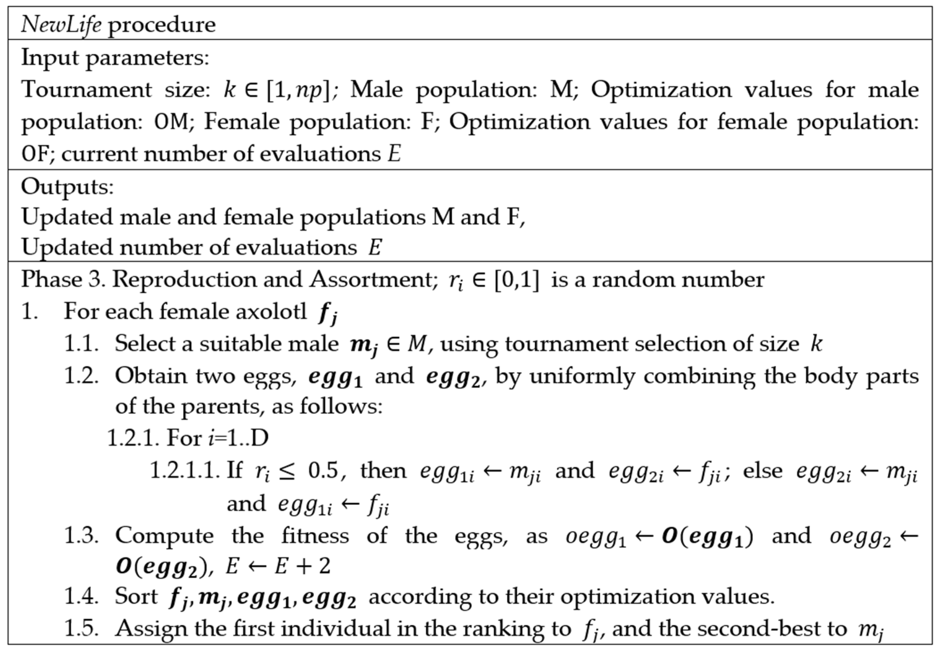
• We consider the females more important, due to the fact that for each female we find the best male according to tournament selection, to obtain the offspring.
• We have an elitist replacement procedure to include new individuals in the population. In such a procedure, the best individual is considered to be a female, and the second-best to be a male. That is, our procedure has the possibility of converting a male into a female, if the male is best.

In the following, we address the experiments made to evaluate MOA for numerical optimization.

4. Results and Discussion

In this section we tested the proposed MAO algorithm, by using several test functions available in the literature. Section 4.1 explains the considered optimization functions, Section 4.2 analyzes the optimization results obtained by MAO and other existing optimization algorithms, Section 4.3 discusses the results and covers the statistical analysis carried out, Section 4.4 discusses the convergence of the Mexican Axolotl Optimization. Finally, Section 4.5 details the main differences of MAO with respect to existing algorithms.

4.1. Optimization Functions

The performance of the MAO needs to be tested. For this, four sets of functions are used, where the first three sets are: unimodal, multimodal, and composite test functions. These sets of functions are included in [20,22], all of them have 10 dimensions. Finally, the fourth set is composed by the functions of the CEC06 2019 “The 100-Digit Challenge” competition [39]. Using several sets of functions allows us to analyze certain aspects of the optimization algorithms.

Unimodal benchmark functions (

Table 1. Definition of unimodal test functions.

Function	Range	Shift Position	Min 1
$TF1\left(x\right)=\sum _{i=1}^n{x}_i^2$	[−100, 100]	[−30, −30, …, −30]	0
$TF2\left(x\right)=\sum _{i=1}^n{x}_i | \prod _{i=1}^n\left|x_i\right|$	[−10, 10]	[−3, −3, …, −3]	0
$TF3\left(x\right)={\displaystyle \sum }_{i=1}^n\left(\sum _{j-1}^i{x}_j{}^2\right)$	[−100, 100]	[−30, −30, …, −30]	0
$TF4\left(x\right)=max\left\{\left|x\right|, 1\le i\le n\right\}$	[−100, 100]	[−30, −30, …, −30]	0
$TF5\left(x\right)=\sum _{i=1}^{n-1}\left[100{\left(x_{i+1}-x_1^2\right)}^2+{\left(x_i-1\right)}^2\right]$	[−30, 30]	[−15, −15, …, −15]	0
$TF6\left(x\right)=\sum _{i=1}^n{\left(\left[x_i+0.5\right]\right)}^2$	[−100, 100]	[−750, …, −750]	0
$TF7\left(x\right)=\sum _{i=1}^{n}i{x}_i^4+random \left[0,1\right]$	[−1.28, 1.28]	[−0.25, …, −0.25]	0

¹ Minimum value of the function.

) have a single minimum solution and are used to determine the capabilities of exploring the search space, and the algorithm’s convergence.

On the other hand, multimodal benchmark functions (

Table 2. Definition of multimodal test functions.

Function	Range	Shift Position	Min 1
$TF8\left(x\right)=\sum _{i=1}^n-x^2\sin \left(\sqrt{\left|x_i\right|}\right)$	[−500, 500]	[−300, …, −300]	−418.9829
$TF9\left(x\right)=\sum _{i=1}^n\left[x_i^2-10\cos \left(2\pi x_i\right)+10\right]$	[−5.12, 5.12]	[−2, −2, …, −2]	0
$TF10\left(x\right)=-20\exp \left(-0.2 \sqrt{\sum _{i=1}^n{x}_i^2}\right)-\exp \left(\frac{1}{n}\sum _{i=1}^n\cos \left(2\pi x_i\right)\right)+20+e$	[−32, 32]	−	0
$TF11\left(x\right)=\frac{1}{4000}\sum _{i=1}^n{x}_i^2-\prod _{i=1}^n\cos \left(\frac{x_i}{\sqrt{i}}\right)+1$	[−600, 600]	[−400, …, −400]	0
$TF12\left(x\right)=\frac{\pi }{n}\left\{10\sin \left(\pi y_1\right)+\sum _{i=1}^{n-1}{\left(y_i-1\right)}^2\left[1+10{\sin }^2\left(\pi y_{i+1}\right)\right]+{\left(y_n-1\right)}^2\right\}+\sum _{i=1}^{n}u\left(x_i,10,100,4\right)$$, \mathrm{where} y_i=1+\frac{x+1}{4}$$, \mathrm{and} u\left(x_i,a,k,m\right)=\left\{\begin{array}{c}k{\left(x_i-a\right)}^m{x}_i>a\\ 0-a<x_i<a\\ k{\left(-x_i-a\right)}^m{x}_i<-a\end{array}\right\}$	[−50, 50]	[−30, −30, …,−30]	0
$TF13\left(x\right)=0.1\left\{{\sin }^2\left(3\pi x1\right)+\sum _{i=1}^n{\left(x_i-1\right)}^2\left[1+{\sin }^2\left(3\pi x_i+1\right)\right]+{\left(x_n-1\right)}^2\left[1+{\sin }^2\left(2\pi x_n\right)\right]\right\}+\sum _{i=1}^{n}u\left(x_i,5,100,4\right)$	[−50, 50]	[−100, …, −100]	0

¹ Minimum value of the function.

) have several optimal solutions. Such functions are used to analyze the ability of the optimization algorithm to avoid local-optimum solutions, and to find one of the global best solutions.

Additionally, the composite benchmark functions (

Table 3. Definition of composite test functions.

Function	Range	Min 1
$\mathit{T}\mathit{F}\mathbf{14}\mathbf{\left(}\mathit{C}\mathit{F}\mathbf{1}\mathbf{\right)}$ $\mathrm{f}1, \mathrm{f}2, \mathrm{f}3 \dots \mathrm{f}10=\mathrm{Sphere} \mathrm{function}$; $\delta 1, \delta 2, \delta 3\dots \delta 10=\left[1,1,1\dots 1\right]$; $\lambda 1, \lambda 2, \lambda 3\dots \lambda 10=\left[\frac{5}{100},\frac{5}{100},\frac{5}{100},\dots \frac{5}{100}\right]$	[−5, 5]	0
$\mathit{T}\mathit{F}\mathbf{15}\mathbf{\left(}\mathit{C}\mathit{F}\mathbf{2}\mathbf{\right)}$ $\mathrm{f}1, \mathrm{f}2, \mathrm{f}3 \dots \mathrm{f}10={\mathrm{Griewank}}^{\prime }\mathrm{s} \mathrm{function}$; $\delta 1, \delta 2, \delta 3\dots \delta 10=\left[1,1,1\dots 1\right]$; $\lambda 1, \lambda 2, \lambda 3\dots \lambda 10=\left[\frac{5}{100},\frac{5}{100},\frac{5}{100},\dots \frac{5}{100}\right]$	[−5, 5]	0
$\mathit{T}\mathit{F}\mathbf{16}\mathbf{\left(}\mathit{C}\mathit{F}\mathbf{3}\mathbf{\right)}$ $\mathrm{f}1, \mathrm{f}2, \mathrm{f}3 \dots \mathrm{f}10={\mathrm{Griewank}}^{\prime }\mathrm{s} \mathrm{function}$; $\delta 1, \delta 2, \delta 3\dots \delta 10=\left[1,1,1\dots 1\right]$; $\lambda 1, \lambda 2, \lambda 3\dots \lambda 10=\left[1,1,1\dots 1\right]$	[−5, 5]	0
$\mathit{T}\mathit{F}\mathbf{17}\mathbf{\left(}\mathit{C}\mathit{F}\mathbf{4}\mathbf{\right)}$ $\mathrm{f}1, \mathrm{f}2={\mathrm{Ackley}}^{\prime }\mathrm{s} \mathrm{function}$$; \mathrm{f}3, \mathrm{f}4={\mathrm{Ackley}}^{\prime }\mathrm{s} \mathrm{function}$$; \mathrm{f}5, \mathrm{f}6={\mathrm{Ackley}}^{\prime }\mathrm{s} \mathrm{function}$$; \mathrm{f}7, \mathrm{f}8={\mathrm{Ackley}}^{\prime }\mathrm{s} \mathrm{function}$$; \mathrm{f}9, \mathrm{f}10={\mathrm{Ackley}}^{\prime }\mathrm{s} \mathrm{function}$$; \delta 1, \delta 2, \delta 3\dots \delta 10=\left[1,1,1\dots 1\right];$$\lambda 1, \lambda 2, \lambda 3\dots \lambda 10=\left[\frac{5}{32},\frac{5}{32},1,1,\frac{5}{0.5},\frac{5}{0.5},\frac{5}{0.5},\frac{5}{0.5},\frac{5}{0.5},\frac{5}{0.5}\right]$	[−5, 5]	0
$\mathit{T}\mathit{F}\mathbf{18}\mathbf{\left(}\mathit{C}\mathit{F}\mathbf{5}\mathbf{\right)}$ $\mathrm{f}1, \mathrm{f}2=\mathrm{Rastrigins} \mathrm{function}$$; \mathrm{f}3, \mathrm{f}4=\mathrm{Weierstrasss} \mathrm{function}$$; \mathrm{f}5, \mathrm{f}6={\mathrm{Griewank}}^{\prime }\mathrm{s} \mathrm{function}$$; \mathrm{f}7, \mathrm{f}8={\mathrm{Ackley}}^{\prime }\mathrm{s} \mathrm{function}$$; \mathrm{f}9, \mathrm{f}10=\mathrm{Sphere} \mathrm{function}$$; \delta 1, \delta 2, \delta 3\dots \delta 10=\left[1,1,1\dots 1\right]$$; \lambda 1, \lambda 2, \lambda 3\dots \lambda 10=\left[\frac{1}{5},\frac{1}{5},\frac{5}{0.5},\frac{5}{0.5},\frac{5}{100},\frac{5}{100},\frac{5}{32},\frac{5}{32},\frac{5}{100},\frac{5}{100}\right]$	[−5, 5]	0
$\mathit{T}\mathit{F}\mathbf{19}\mathbf{\left(}\mathit{C}\mathit{F}\mathbf{6}\mathbf{\right)}$ $\mathrm{f}1, \mathrm{f}2=\mathrm{Rastrigins} \mathrm{function}$$; \mathrm{f}3, \mathrm{f}4=\mathrm{Weierstrasss} \mathrm{function}$$; \mathrm{f}5, \mathrm{f}6={\mathrm{Griewank}}^{\prime }\mathrm{s} \mathrm{function}$$; \mathrm{f}7, \mathrm{f}8={\mathrm{Ackley}}^{\prime }\mathrm{s} \mathrm{function}$$; \mathrm{f}9, \mathrm{f}10=\mathrm{Sphere} \mathrm{function}$$; \delta 1, \delta 2, \delta 3\dots \delta 10=\left[0.1,0.2,0.3,0.4,0.5,0.6,0.7,0.8,0.9,1\right]$$; \lambda 1, \lambda 2, \lambda 3\dots \lambda 10=\left[0.1\ast \frac{1}{5},0.2\ast \frac{1}{5},0.3\ast \frac{5}{0.5},0.4\ast \frac{5}{0.5},0.5\ast \frac{5}{100},0.6\ast \frac{5}{100},0.7\ast \frac{5}{32},0.8\ast \frac{5}{32},0.9\ast \frac{5}{100},1\ast \frac{5}{100}\right]$	[−5, 5]	0

¹ Minimum value of the function.

) are complex functions used to simulated real-world complexity. Such functions are often shifted, rotated, and biased versions of other test functions. Usually, they also have singular shapes.

Last but not least, the functions of the CEC06 competition [39] are well-known complex functions, usually used in international competitions.

Table 4. Definition of CEC06 2019 “The 100-Digit Challenge” test functions.

Function	Dimensions	Range	Min 1
Storn’s Chebyshev polynomial fitting problem	9	[−8192, 8192]	1
Inverse Hilbert matrix problem	16	[−16,384, 16,384]	1
Lennard-Jones minimum energy cluster	18	[−4, 4]	1
Rastrigin’s function	10	[−100, 100]	1
Griewangk’s function	10	[−100, 100]	1
Weierstrasss function	10	[−100, 100]	1
Modified Schewefel’s function	10	[−100, 100]	1
Expanded Schafeer’s F6 function	10	[−100, 100]	1
Happy Cat function	10	[−100, 100]	1
Ackley function	10	[−100, 100]	1

¹ Minimum value of the function.

shows the generalities of those functions.

4.2. Optimization Results of the Compared Algorithms

We selected some of the best-performing algorithms for the abovementioned functions, according to the research of [22]. We use the MATLAB [40] source code for the compared optimization algorithms, which are available at www.mathworks.com (accessed on 31 March 2021).

The selected algorithms (in alphabetical order) are: Artificial Bee Colony (ABC) [26], Cuckoo Search (CS) [15], Differential Evolution (DE) [6], Firefly Algorithm (FA) [17,18], Fitness Dependent Optimizer (FDO) algorithm [22], Monarch Butterfly Optimization (MBO) [24], Slime Mould Algorithm (SMA) [25] and Whale Optimization Algorithm (WOA) [27].

Table 5. Averaged results of the optimization algorithms over the benchmark functions.

Set	Function	ABC	CS	DE	FA	FDO	MBO	SMA	WOA	MAO
Unimodal	F1	5447.7037	9165.9901	8587.4237	2936.3110	2855.3899	2997.0703	13.0903	234.8699	321.0370
	F2	2.8086	31.3204	35.0858	14.5341	13.8453	13.6921	0.3195	3.2792	4.1843
	F3	7228.5989	9879.7702	10,826.8313	4258.6261	5174.2327	6729.9519	5245.1086	13,758.8168	700.1304
	F4	57.9899	54.8784	59.7082	29.7369	25.2446	23.4809	0.3670	41.7093	12.3571
	F5	2.68 × 106	1.10 × 107	9.71 × 106	1.23 × 106	3.12 × 106	4.40 × 106	13.1924	3.51 × 104	1.84 × 104
	F6	5928.5177	9269.7192	7336.3097	3043.6261	2771.3385	3193.3915	3.0798	246.8890	266.5308
	F7	1.2196	2.3582	2.8935	0.6749	1.1486	2.5256	0.1911	0.2530	0.0484
Multimodal	F8	−2407.4569	−1809.7610	−1950.2114	−1531.2946	−1483.9961	−3132.3800	−3293.9270	−2635.7968	−2843.8943
	F9	70.2922	91.3020	95.3271	67.2274	55.1742	44.5630	15.3040	56.0142	25.3499
	F10	17.9524	18.7192	19.4404	15.1343	10.1403	11.3944	0.5564	7.3438	7.1662
	F11	46.1170	83.3698	71.7901	27.2379	24.3820	22.7500	0.4801	2.5929	3.7582
	F12	2.36 × 106	1.42 × 107	1.62 × 107	1.22 × 105	1.56 × 106	1.99 × 106	2.5396	5.96 × 103	5.95
	F13	7.54 × 106	5.21 × 107	5.64 × 107	2.12 × 106	9.22 × 106	1.17 × 106	1.0523	3.03 × 104	3.28 × 103
Composite	F14	342.3150	354.0967	410.7029	758.6487	968.2830	393.5150	429.0229	395.7099	473.1349
	F15	476.2411	463.9622	468.3889	821.8865	1048.0255	478.9110	513.0348	457.5810	507.2991
	F16	1072.7264	1052.7694	1056.7774	1491.2869	1393.0906	1087.9062	1062.6645	1114.6494	1147.8570
	F17	990.3510	1003.4222	1026.9885	1077.1571	1050.0625	1001.3681	904.2288	999.8535	952.0442
	F18	420.8507	424.6245	442.7791	894.0803	1136.6270	420.0096	508.7819	447.0013	524.1615
	F19	1003.9296	996.0488	978.5206	974.7888	951.7356	933.2716	874.2914	933.4341	905.2780
Competition	CEC01	6.27 × 1011	1.13 × 1012	6.26 × 1011	1.04 × 1012	3.96 × 1011	8.13 × 1011	8.17 × 1011	1.01 × 1012	4.11 × 1010
	CEC02	10,208.4315	8666.1661	4254.8599	4408.7645	4833.2511	7174.2428	41.9309	479.6424	424.2248
	CEC03	12.7058	12.7047	12.7039	12.7043	12.7037	12.7036	12.7035	12.7026	12.7026
	CEC04	8564.8124	16,171.5930	9055.5641	11,536.6751	4962.4534	7862.3602	17,307.1928	5700.3273	4460.3403
	CEC05	4.4837	5.4179	3.9627	3.8751	2.8207	3.4589	5.6967	3.1687	2.6745
	CEC06	11.8186	13.0760	13.3387	14.3070	13.5259	11.4701	13.0106	13.1277	12.5090
	CEC07	1016.2961	1318.4455	1425.1217	1635.1259	1506.3325	1057.3337	1204.1217	1275.5805	1184.9008
	CEC08	6.9177	7.2169	7.4573	7.5103	7.0885	6.9756	7.4529	7.1778	6.8954
	CEC09	2013.8642	3939.6893	2682.6881	1773.0340	1059.9142	1321.8686	4199.2309	1043.8402	431.0717
	CEC10	20.6068	20.7581	20.8089	20.8308	20.8116	20.5595	20.7914	20.7122	20.6511

shows the results for all compared functions. Each algorithm was executed 30 times, and the results were averaged.

We established 500 evaluations of the objective function as a termination criterion for all algorithms. It is important to mention that using just 500 evaluations (the usual number in competitions [41]) as a termination criterion is a very restrictive one, which gives the optimization algorithms little time to travel through the search space. The performance with such a small number estimates the ability of the algorithm to focus on promissory areas of the search space in just few iterations.

We implemented the proposed Mexican Axolotl Optimization (MAO) algorithm in MATLAB [40] it the version 9.8 (R2020a), and we executed all the experiments in a desk computer with Windows Professional operating system, with Intel^® Core™ i7-6700 CPU 3.40 GHz processor, 16 GB of RAM, and a Nvidia GeForce GTX 1070 graphics card.

We used the suggested parameters as in the original source code for the literature algorithms (

Table 6. Parameters for the literature algorithms.

Algorithm	Parameters 1
ABC	Number of food sources: 30; Maximum number of failures which lead to the elimination: Number of food sources * dimension
CS	Number of nests: 30; Discovery rate of alien eggs/solutions: 10−5
DE	Population Size: 30; Crossover probability: 0.8; Scaling factor: 0.85
FA	Number of Fireflies: 30; Alpha: 0.5; Betamin: 0.2; Gamma: 1.0
FDO	Scout bee number: 30; Weight Factor: 0.0
MAO	Total population size: 30; damage probability dp = 0.5; regeneration probability rp = 0.1; tournament size k = 3; differentiation constant $\lambda =0.5$.
MBO	Total population size: 30; The percentage of population for MBO: 5/12; Elitism parameter: 2.0; Max Step size: 1.0; 12 months in a year: 1.2
SMA	Number of search agent: 30; z: 0.03
WOA	Number of search agents

¹ As in the MATLAB code publicly available at www.mathworks.com (accessed on 31 March 2021).

). For MAO, we use similar parameters (Table 6). We made the source code of the proposed MAO available at (https://la.mathworks.com/matlabcentral/fileexchange/88451-mexican-axolotl-optimization-a-novel-bioinspired-heuristic) (accessed on 31 March 2021).

As shown in Table 5, the best algorithm for unimodal and multimodal functions was SMA. However, this algorithm includes a parameter generated randomly, which decreases linearly from one to zero [25]. This parameter is used to update the solutions if a random number in [0, 1] is lower than a value p, computed using a hyperbolic tangent. That is, the SMA algorithm biases its solutions to be close to zero.

The proposed MAO is particularly good with unimodal and multimodal optimization functions (best in two functions and second-best in four functions) as well as for competence functions (best in six of 10). However, for composite functions, it has an average performance.

In addition, we consider that our proposal is particularly good for few function evaluations, because we obtained very good results with just 500 evaluations of the objective functions.

4.3. Statistical Tests

We used the Friedman test [42], followed by the Holm’s post hoc test [43], to determine if the differences in performance of MAO with respect to the other optimization algorithms compared were significant or not. Both tests are recommended in [44]. We used the KEEL software [45] for computing both tests.

We set as null hypothesis H0 that there were no significant differences between the compared algorithm, and as H1 that there were significant differences in their performance. We set a significance level $\alpha =0.05$, for a 95% of confidence.

Table 7. Ranking obtained by the Friedman test.

Algorithm.	Ranking
MAO	2.7069
SMA	3.4483
WOA	3.8448
MBO	4.1724
ABC	5.1724
FDO	5.5517
FA	6.4828
CS	6.7931
DE	6.8276

shows the ranking obtained by the Friedman test, with MAO being the best-ranked algorithms. The test obtained a p-value of 0.00, rejecting the null hypothesis. In

Table 8. Results of the Holm’s test while comparing MAO and other optimization algorithms.

i	Algorithm	Z	p-Value	Holm
8	DE	5.729586	0.000000	0.006250
7	CS	5.68164	0.000000	0.007143
6	FA	5.250123	0.000000	0.008333
5	FDO	3.955572	0.000076	0.010000
4	ABC	3.428163	0.000608	0.012500
3	MBO	2.037719	0.041578	0.016667
2	WOA	1.582229	0.113597	0.025000
1	SMA	1.030846	0.302613	0.050000

, we show the results for the Holm’s test comparing MAO with respect to literature algorithms. The Holm procedure rejects those hypotheses that have an unadjusted p-value lower than or equal to 0.016667.

The statistical tests reject the null hypothesis for ABC, FDO, FA, CS and DE, resulting in MAO having significant differences with respect to those optimization algorithms. As MAO was the best-ranked algorithm, we can conclude that the differences favor our proposal. For the SMA, WOA and MBO algorithms, the test did not reject the null hypothesis. These tests support the usefulness of the proposed Mexican Axolotl Optimization algorithm.

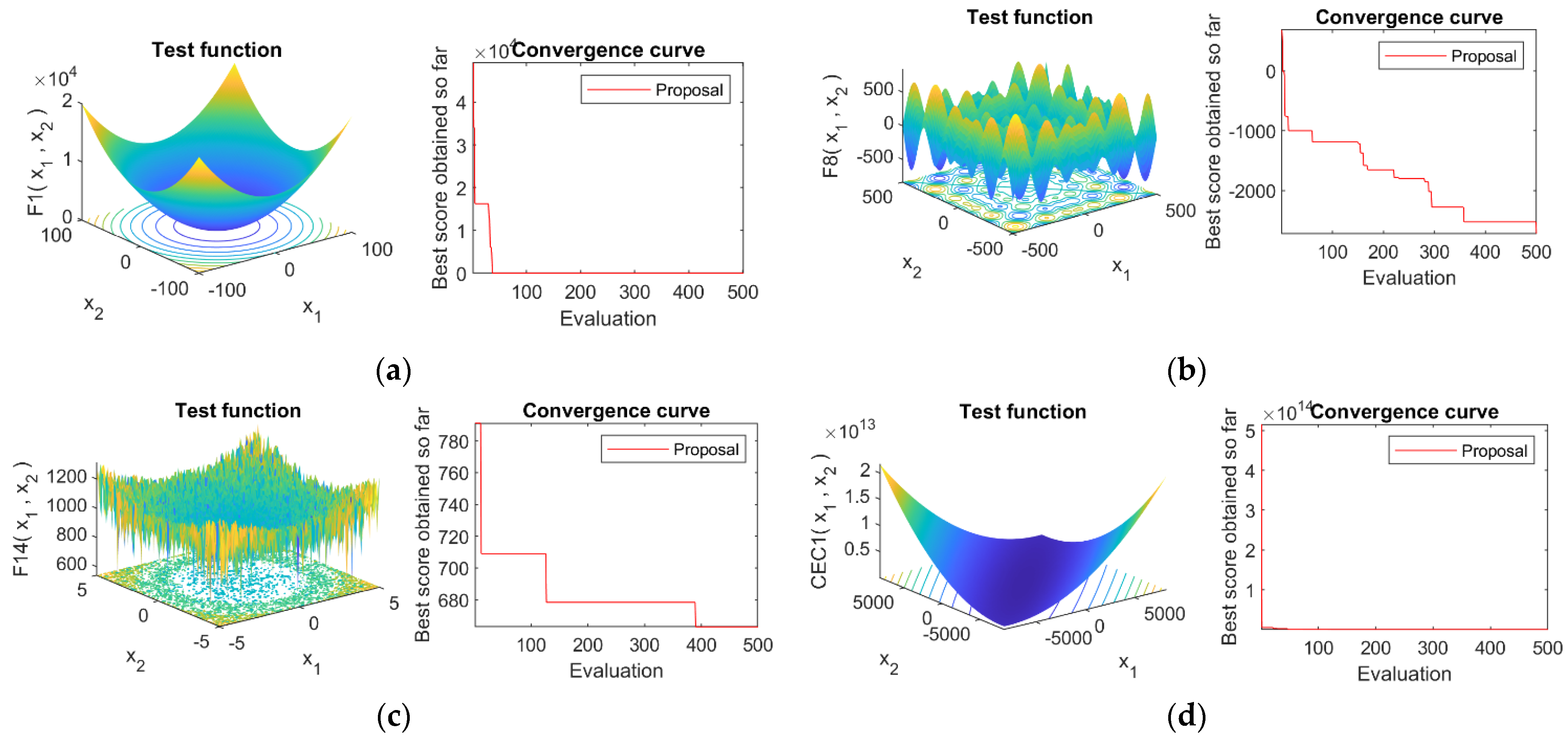
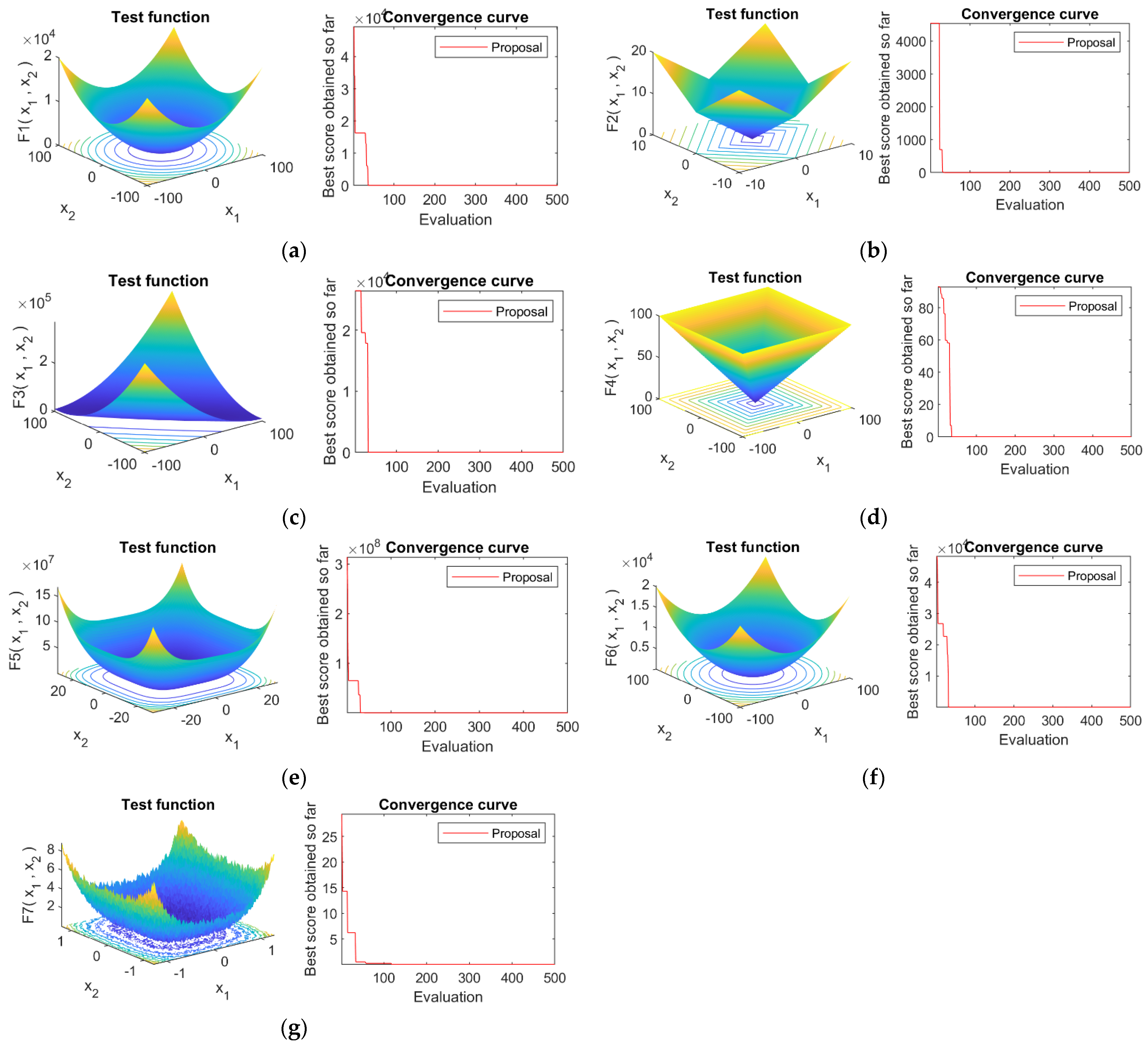
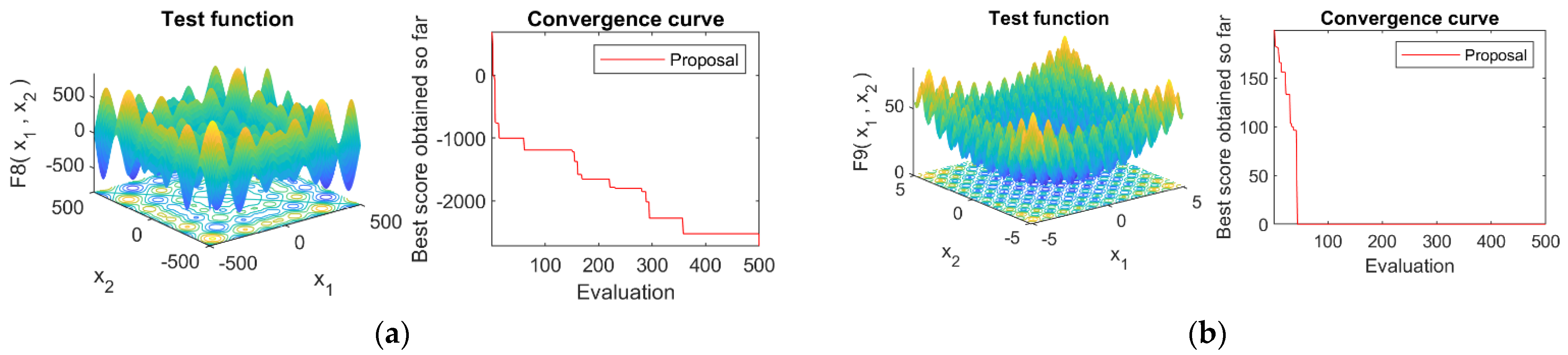
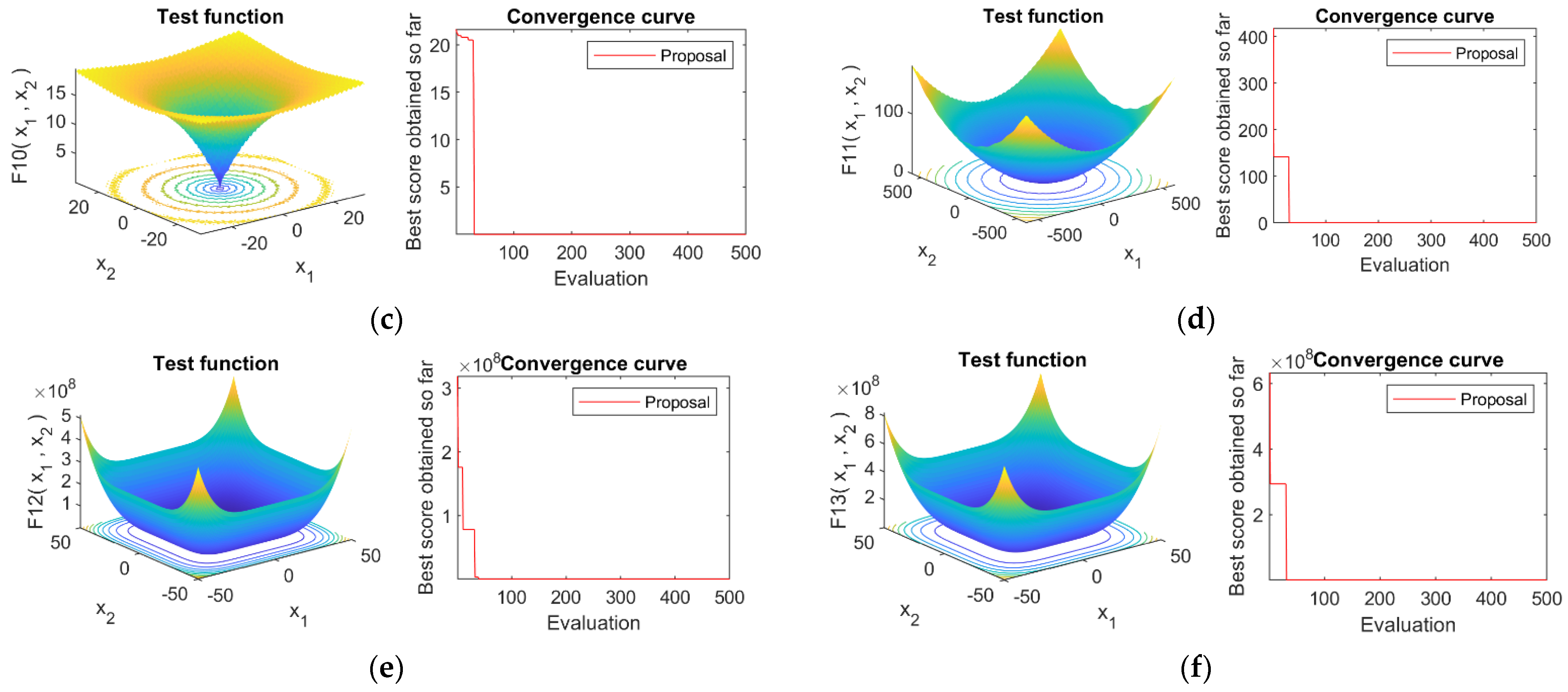
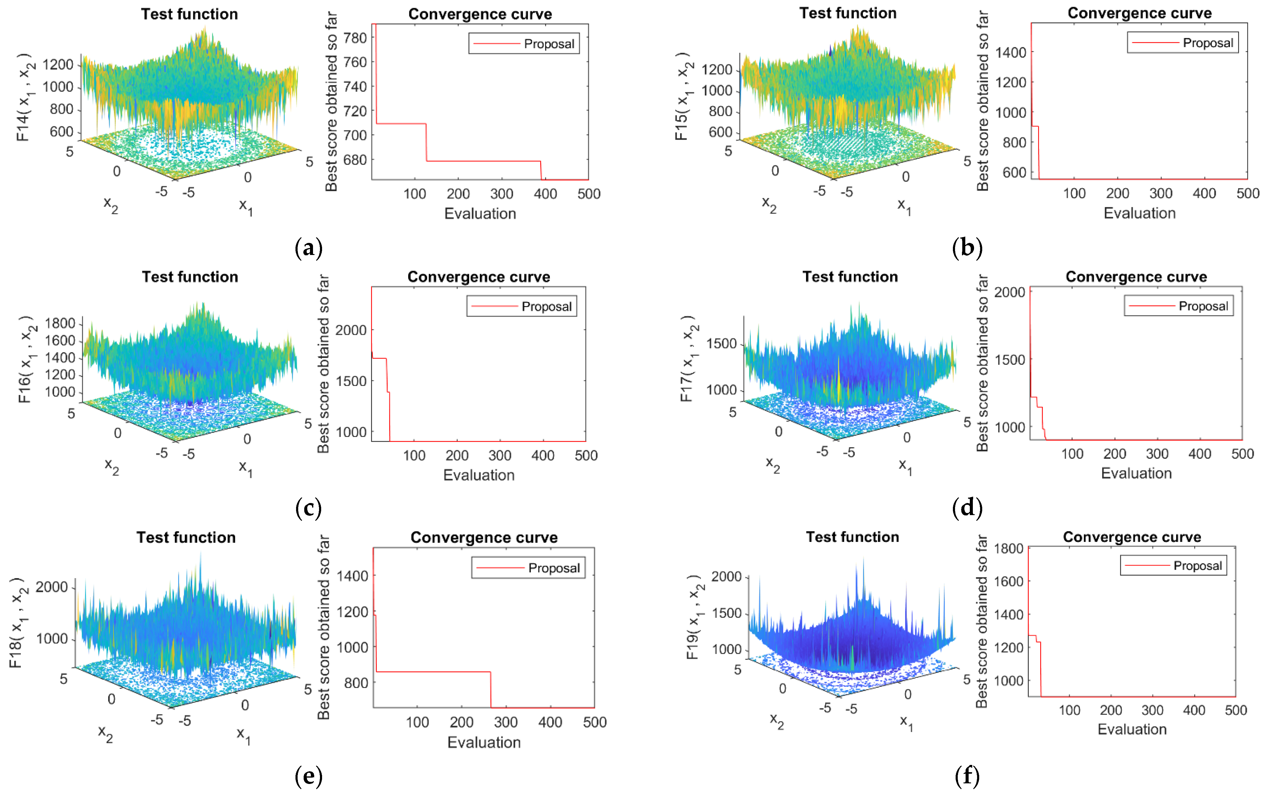
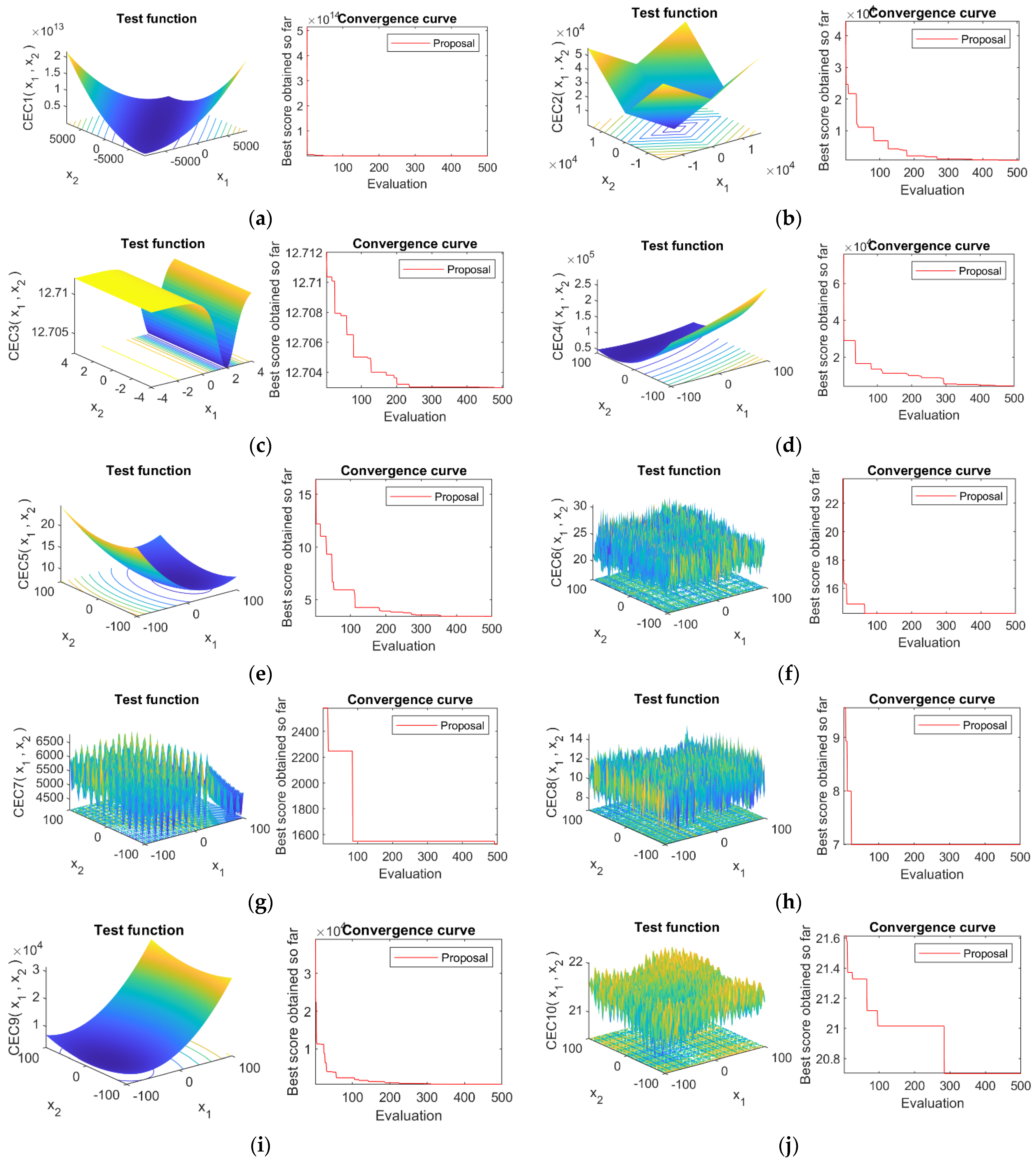
4.4. Convergence Analysis

In this section, we analyze the convergence of the proposed MAO, for the benchmark functions analyzed. We plot the optimization results obtained, with respect to the number of evaluations of the objective function. In Figure 6, we show the results for the first function of each test set, i.e., functions F1, F8, F14, and cec01. The theoretical demonstration of the MAO algorithm’s convergence is left for future work.

As shown, the proposed MAO algorithm converges quickly towards a minimum value; it supports the idea that the heuristic procedure focuses on promissory areas of the search space, which allows MAO to find good solutions to the problem. Figure 6 also shows the shape of the test functions, verifying the complexity of the corresponding search space. In Appendix A we give the convergence curves of MAO for the four sets of test functions (Figure A1, Figure A2, Figure A3 and Figure A4).

For example, we can see that MAO was trapped in a local minimum for function F14 during several evaluations. However, it was able to escape the local minimum fast enough. Again, we want to clarify that using 500 evaluations [41] is challenging for optimization algorithms.

4.5. Main differences of MAO with Respect Other Bioinspired Algorithms

From the conceptual point of view, our method has the advantage of using a population separately in two subpopulations (males and females), which evolve separately in Phase 1 (Transition from larvae to adult state) and Phase 2 (Injury and restoration). This allows MAO to search several areas of the search space, without the risk of premature convergence. In Phase 3 (Reproduction and Assortment), we obtain novel individuals, and we have the advantage of preserving the best ones, by assigning the best individual to the female subpopulation, and the second-best to the male subpopulation. Due to the parents can change population (if the parents are better than the offspring and the male parent is better than the female parent), MAO can introduce novel information into the subpopulation, which also diminishes the risk of premature convergence towards the local minimum.

In addition, our proposal IS NOT BIASED to obtain solutions with zero-valued components, nor towards any other specific values. This makes MAO suitable for a wide range set of optimization problems, in which the optimum values of the function are not near zero.

We think that these characteristics make MAO suitable for numerical optimization with low evaluation numbers, as proven in the experimental comparisons.

5. Conclusions

Our novel bioinspired heuristic is, in fact, a metaheuristic. It is not simply a rule; it is a “scenario” situated at a metalevel when compared to the optimization problem. The results obtained in the experiments carried out in this research show that the proposed MAO is very good with unimodal and multimodal optimization functions (best in five of seven and four of six, respectively) and has a good performance for competence functions (best in seven of ten). However, for composite functions, it has an average performance, being the best in just one out of six functions. Additionally, the Friedman test, followed by the Holm’s post hoc test, supports the usefulness of the proposed Mexican Axolotl Optimization algorithm in optimization problems.

It should be noted that in addition to MAO, some of the most representative computational intelligence algorithms can be used to face the problems included in this paper, like monarch butterfly optimization (MBO) [24], earthworm optimization algorithm (EWA) [46], elephant herding optimization (EHO) [47], moth search (MS) algorithm [48], Slime mould algorithm (SMA) [25], and Harris hawks optimization (HHO) [49].

As future work, we propose to perform comparative studies of MAO against the performance of some of the newest proposed methods, such as krill herd, earthworm optimization algorithm (EWA), elephant herding optimization (EHO), moth search (MS) algorithm, and Harris hawks optimization (HHO). In addition, we want to perform novel experiments to determine the contribution of each phase of the proposed MAO over the final result, as well as the adequate parameter values for MAO, to give the scientific community guidelines for their selection. Finally, as stated before, the theoretical demonstration of the MAO algorithm’s convergence is left for future work.

References

1. Dinov, I.D. Function Optimization. In Data Science and Predictive Analytics; Springer: Cham, Switzerland, 2018; pp. 735–763. [Google Scholar]
2. Flood, M.M. The traveling-salesman problem. Oper. Res. 1956, 4, 61–75. [Google Scholar] [CrossRef]
3. Beckers, R.; Deneubourg, J.; Gross, S. Trail and U-turns in the Selection of the Shortest Path by the Ants. J. Theor. Biol. 1992, 159, 397–415. [Google Scholar] [CrossRef]
4. Holland, J.H. Genetic algorithms and the optimal allocation of trials. SIAM J. Comput. 1973, 2, 88–105. [Google Scholar] [CrossRef]
5. Koza, J.R. Genetic Programming: A Paradigm for Genetically Breeding Populations of Computer Programs to Solve Problems; Stanford University, Department of Computer Science: Stanford, CA, USA, 1990; Volume 34. [Google Scholar]
6. Storn, R.; Price, K. Differential evolution—A simple and efficient heuristic for global optimization over continuous spaces. J. Glob. Optim. 1997, 11, 341–359. [Google Scholar] [CrossRef]
7. Fan, X.; Sayers, W.; Zhang, S.; Han, Z.; Ren, L.; Chizari, H. Review and classification of bio-inspired algorithms and their applications. J. Bionic Eng. 2020, 17, 611–631. [Google Scholar] [CrossRef]
8. Ullah, I.; Hussain, I.; Singh, M. Exploiting grasshopper and cuckoo search bio-inspired optimization algorithms for industrial energy management system: Smart industries. Electronics 2020, 9, 105. [Google Scholar] [CrossRef] [Green Version]
9. Abdelaziz, F.B.; Alaya, H.; Dey, P.K. A multi-objective particle swarm optimization algorithm for business sustainability analysis of small and medium sized enterprises. Ann. Oper. Res. 2020, 293, 557–586. [Google Scholar] [CrossRef] [Green Version]
10. Phan, A.V.; Le Nguyen, M.; Bui, L.T. Feature weighting and SVM parameters optimization based on genetic algorithms for classification problems. Appl. Intell. 2017, 46, 455–469. [Google Scholar] [CrossRef]
11. Santos, P.; Macedo, M.; Figueiredo, E.; Santana, C.J.; Soares, F.; Siqueira, H.; Maciel, A.; Gokhale, A.; Bastos-Filho, C.J. Application of PSO-based clustering algorithms on educational databases. In Proceedings of the 2017 IEEE Latin American Conference on Computational Intelligence (LA-CCI), Arequipa, Peru, 8–10 November 2017; pp. 1–6. [Google Scholar]
12. Pant, M.; Zaheer, H.; Garcia-Hernandez, L.; Abraham, A. Differential evolution: A review of more than two decades of research. Eng. Appl. Artif. Intell. 2020, 90, 103479. [Google Scholar]
13. Binitha, S.; Sathya, S.S. A survey of bio inspired optimization algorithms. Int. J. Soft Comput. Eng. 2012, 2, 137–151. [Google Scholar]
14. Almufti, S.; Marqas, R.; Ashqi, V. Taxonomy of bio-inspired optimization algorithms. J. Adv. Comput. Sci. Technol. 2019, 8, 23. [Google Scholar] [CrossRef] [Green Version]
15. Yang, X.-S.; Deb, S. Cuckoo search via Lévy flights. In Proceedings of the 2009 World Congress on Nature & Biologically Inspired Computing (NaBIC), Kitakyushu, Japan, 15–17 December 2010; pp. 210–214. [Google Scholar]
16. Yang, X.-S.; Deb, S. Engineering optimisation by cuckoo search. Int. J. Math. Model. Numer. Optim. 2010, 1, 330–343. [Google Scholar] [CrossRef]
17. Yang, X.-S. Firefly algorithm. Nat. Inspired Metaheuristic Algorithms 2008, 20, 79–90. [Google Scholar]
18. Yang, X.-S. Firefly algorithms for multimodal optimization. In Proceedings of the International Symposium on Stochastic Algorithms, Sapporo, Japan, 26–28 October 2009; pp. 169–178. [Google Scholar]
19. Kumar, V.; Kumar, D. A Systematic Review on Firefly Algorithm: Past, Present, and Future. Arch. Comput. Methods Eng. 2020, 1–23. [Google Scholar] [CrossRef]
20. Mirjalili, S. Dragonfly algorithm: A new meta-heuristic optimization technique for solving single-objective, discrete, and multi-objective problems. Neural Comput. Appl. 2016, 27, 1053–1073. [Google Scholar] [CrossRef]
21. Meraihi, Y.; Ramdane-Cherif, A.; Acheli, D.; Mahseur, M. Dragonfly algorithm: A comprehensive review and applications. Neural Comput. Appl. 2020, 32, 16625–16646. [Google Scholar] [CrossRef]
22. Abdullah, J.M.; Ahmed, T. Fitness dependent optimizer: Inspired by the bee swarming reproductive process. IEEE Access 2019, 7, 43473–43486. [Google Scholar] [CrossRef]
23. Eberhart, R.; Kennedy, J. Particle swarm optimization. In Proceedings of the IEEE International Conference on Neural Networks, Perth, Australia, 27 November–1 December 1995; pp. 1942–1948. [Google Scholar]
24. Wang, G.-G.; Deb, S.; Cui, Z. Monarch butterfly optimization. Neural Comput. Appl. 2019, 31, 1995–2014. [Google Scholar] [CrossRef] [Green Version]
25. Li, S.; Chen, H.; Wang, M.; Heidari, A.A.; Mirjalili, S. Slime mould algorithm: A new method for stochastic optimization. Future Gener. Comput. Syst. 2020, 111, 300–323. [Google Scholar] [CrossRef]
26. Karaboga, D.; Basturk, B. A powerful and efficient algorithm for numerical function optimization: Artificial bee colony (ABC) algorithm. J. Glob. Optim. 2007, 39, 459–471. [Google Scholar] [CrossRef]
27. Mirjalili, S.; Lewis, A. The whale optimization algorithm. Adv. Eng. Softw. 2016, 95, 51–67. [Google Scholar] [CrossRef]
28. Gresens, J. An introduction to the Mexican axolotl (Ambystoma mexicanum). Lab Anim. 2004, 33, 41–47. [Google Scholar] [CrossRef] [PubMed]
29. Voss, S.R.; Woodcock, M.R.; Zambrano, L. A tale of two axolotls. BioScience 2015, 65, 1134–1140. [Google Scholar] [CrossRef] [PubMed]
30. Cortázar, J. End of the Game; In Spanish, Final del Juego; HarperCollins: New York, NY, USA, 1956. [Google Scholar]
31. Herbert, F. Dune; Chilton Company: Boston, MA, USA, 1965. [Google Scholar]
32. Tank, P.W.; Carlson, B.M.; Connelly, T.G. A staging system for forelimb regeneration in the axolotl, Ambystoma mexicanum. J. Morphol. 1976, 150, 117–128. [Google Scholar] [CrossRef] [Green Version]
33. Demircan, T.; Hacıbektaşoğlu, H.; Sibai, M.; Fesçioğlu, E.C.; Altuntaş, E.; Öztürk, G.; Süzek, B.E. Preclinical molecular signatures of spinal cord functional restoration: Optimizing the metamorphic axolotl (Ambystoma mexicanum) model in regenerative medicine. OMICS J. Integr. Biol. 2020, 24, 370–378. [Google Scholar] [CrossRef]
34. Vieira, W.A.; Wells, K.M.; McCusker, C.D. Advancements to the axolotl model for regeneration and aging. Gerontology 2020, 66, 212–222. [Google Scholar] [CrossRef]
35. Nowoshilow, S.; Schloissnig, S.; Fei, J.-F.; Dahl, A.; Pang, A.W.; Pippel, M.; Winkler, S.; Hastie, A.R.; Young, G.; Roscito, J.G. The axolotl genome and the evolution of key tissue formation regulators. Nature 2018, 554, 50–55. [Google Scholar] [CrossRef] [Green Version]
36. Pietsch, P.; Schneider, C.W. Vision and the skin camouflage reactions of Ambystoma larvae: The effects of eye transplants and brain lesions. Brain Res. 1985, 340, 37–60. [Google Scholar] [CrossRef]
37. Griffiths, R.A.; Graue, V.; Bride, I.G. The axolotls of Lake Xochimilco: The evolution of a conservation programme. Axolotl News 2003, 30, 12–18. [Google Scholar]
38. Khattak, S.; Murawala, P.; Andreas, H.; Kappert, V.; Schuez, M.; Sandoval-Guzmán, T.; Crawford, K.; Tanaka, E.M. Optimized axolotl (Ambystoma mexicanum) husbandry, breeding, metamorphosis, transgenesis and tamoxifen-mediated recombination. Nat. Protoc. 2014, 9, 529. [Google Scholar] [CrossRef] [PubMed]
39. Price, K.; Awad, N.; Ali, M.; Suganthan, P. Problem Definitions and Evaluation Criteria for the 100-Digit Challenge Special Session and Competition on Single Objective Numerical Optimization; Technical Report; Nanyang Technological University: Singapore, 2018. [Google Scholar]
40. MATLAB. Matlab, version 9.8 (R2020a); The MathWorks Inc.: Natick, MA, USA, 2020. [Google Scholar]
41. Chen, Q.; Liu, B.; Zhang, Q.; Liang, J.; Suganthan, P.; Qu, B. Problem Definitions and Evaluation Criteria for CEC 2015 Special Session on Bound Constrained Single-Objective Computationally Expensive Numerical Optimization; Technical Report; Computational Intelligence Laboratory, Zhengzhou University: Zhengzhou, China; Nanyang Technological University: Singapore, 2014. [Google Scholar]
42. Friedman, M. A comparison of alternative tests of significance for the problem of m rankings. Ann. Math. Stat. 1940, 11, 86–92. [Google Scholar] [CrossRef]
43. Holm, S. A simple sequentially rejective multiple test procedure. Scand. J. Stat. 1979, 6, 65–70. [Google Scholar]
44. Derrac, J.; García, S.; Molina, D.; Herrera, F. A practical tutorial on the use of nonparametric statistical tests as a methodology for comparing evolutionary and swarm intelligence algorithms. Swarm Evol. Comput. 2011, 1, 3–18. [Google Scholar] [CrossRef]
45. Triguero, I.; González, S.; Moyano, J.M.; García, S.; Alcalá-Fdez, J.; Luengo, J.; Fernández, A.; del Jesús, M.J.; Sánchez, L.; Herrera, F. KEEL 3.0: An open source software for multi-stage analysis in data mining. Int. J. Comput. Intell. Syst. 2017, 10, 1238–1249. [Google Scholar] [CrossRef] [Green Version]
46. Wang, G.G.; Deb, S.; Coelho, L.D.S. Earthworm optimisation algorithm: A bio-inspired metaheuristic algorithm for global optimisation problems. Int. J. Bio Inspired Comput. 2018, 12, 1–22. [Google Scholar] [CrossRef]
47. Wang, G.G.; Deb, S.; Coelho, L.D.S. Elephant herding optimization. In Proceedings of the 2015 3rd International Symposium on Computational and Business Intelligence (ISCBI), Bali, Indonesia, 7–9 December 2015; pp. 1–5. [Google Scholar]
48. Wang, G.G. Moth search algorithm: A bio-inspired metaheuristic algorithm for global optimization problems. Memetic Comput. 2018, 10, 151–164. [Google Scholar] [CrossRef]
49. Heidari, A.A.; Mirjalili, S.; Faris, H.; Aljarah, I.; Mafarja, M.; Chen, H. Harris hawks optimization: Algorithm and applications. Future Gener. Comput. Syst. 2019, 97, 849–872. [Google Scholar] [CrossRef]
Figure 1. Pseudocode of the Transition procedure, corresponding to the Transition from larvae to adult state phase in the Mexican Axolotl Optimization (MAO) algorithm.
Mathematics 09 00781 g001
Figure 2. Pseudocode of the Accidents procedure, corresponding to the Injury and restoration state phase in the MAO algorithm.
Mathematics 09 00781 g002
Figure 3. Pseudocode of the NewLife procedure, corresponding to the Reproduction and Assortment phase in the MAO algorithm of the proposed Mexican Axolotl Optimization.
Mathematics 09 00781 g003
Figure 4. Reproduction in the MAO. (a) Male parent, (b) female parent, (c) random numbers generated to uniformly distribute the parents’ information, and (d) the resulting offspring
Mathematics 09 00781 g004
Figure 5. Pseudocode of the proposed Mexican Axolotl Optimization.
Mathematics 09 00781 g005
Figure 6. Convergence of the Mexican Axolotl Optimization for some benchmark functions (a) F1 test function (b) F8 test function (c) F14 test function, and (d) CEC01 test function.
Mathematics 09 00781 g006