Article

A Concretization of an Approximation Method for Non-Affine Fractal Interpolation Functions

by
Alexandra Băicoianu
1,
Cristina Maria Păcurar
1 and
Marius Păun
2,*
1
Department of Mathematics and Computer Science, Faculty of Mathematics and Computer Science, Transilvania University of Braşov 50, Iuliu Maniu Str., 500090 Braşov, Romania
2
Department of Forest Engineering, Forest Management Planing and Terrestrial Measurements, Faculty of Silviculture and Forest Engineering, Transilvania University of Braşov, 1 Şirul Beethoven, 500123 Braşov, Romania
*
Author to whom correspondence should be addressed.
Mathematics 2021, 9(7), 767; https://doi.org/10.3390/math9070767
Submission received: 10 March 2021 / Revised: 26 March 2021 / Accepted: 28 March 2021 / Published: 1 April 2021

Abstract

:
The present paper concretizes the models proposed by S. Ri and N. Secelean. S. Ri proposed the construction of the fractal interpolation function (FIF) considering finite systems consisting of Rakotch contractions, but produced no concretization of the model. N. Secelean considered countable systems of Banach contractions to produce the fractal interpolation function. Based on the abovementioned results, in this paper, we propose two different algorithms to produce the fractal interpolation functions both in the affine and non-affine cases. The theoretical context we were working in suppose a countable set of starting points and a countable system of Rakotch contractions. Due to the computational restrictions, the algorithms constructed in the applications have the weakness that they use a finite set of starting points and a finite system of Rakotch contractions. In this respect, the attractor obtained is a two-step approximation. The large number of points used in the computations and the graphical results lead us to the conclusion that the attractor obtained is a good approximation of the fractal interpolation function in both cases, affine and non-affine FIFs. In this way, we also provide a concretization of the scheme presented by C.M. Păcurar.

1. Introduction

The notion of fractal interpolation has been introduced by Barnesley in [1] (see also [2]) and it represents a different interpolation method, which results in functions that are continuous, but not necessarily differentiable at every point. The fractal interpolation function (FIF) is a continuous function with real values, which interpolates a given set of data
{ ( x i , y i ) [ x 0 , x N ] × R , i = { 0 , , N 1 } }
(i.e., f ( x i ) = y i for all i { 0 , , N 1 } ), where x i are sorted in an ascending order such that its graph is the attractor of an iterated function system.
The significance of FIFs is emphasized by the numerous research directions that have been broadly studied ever since they were introduced. Among these directions, we mention the hidden variable fractal interpolation, which was introduced by Barnsley et al. (see [3]) and generates functions which are not self-referential; thus, being much more less restrictive (see [4,5,6]), the extension to a countable iterated function systems (a notion introduced in [7,8,9]) to obtain the corresponding FIFs (see [10,11]) and the replacement of the fixed point result (Banach fixed point theorem), which guarantees the existence of the FIF with different fixed point results (see [12,13,14,15]).
Among the different types of FIFs existing in the literature, there were studied affine FIFs (see [1]), but also non-affine FIFs (see [16]). However, if for the affine case, there have been studies undertaken towards the computational part (see [17,18,19,20,21]), as far as we know, there have not yet been any studies related to non-affine FIFs in this respect.
The aim of the present paper is to offer a concretization of an approximation method for non-affine fractal interpolation functions. Starting from the results in [8,12], in this paper, we propose two different algorithms to produce the fractal interpolation functions in both cases affine and non-affine FIFs. The theoretical context we were working in, suppose a countable set of starting points and a countable system of Rakotch contractions. Due to the computational restrictions the built algorithms, in applications, have the weakness that they uses a finite set of starting points and a finite system of Rakotch contractions. With this respect, the attractor obtained is a two-step approximation. The big amount of points used in the computations and the graphical results lead us to the conclusion that the attractor obtained is a good approximation of the fractal interpolation function in both affine and non-affine cases. In this way, we also provide a concretization of the scheme presented by C.M. Păcurar (see [15]).
In this study, we want to solve also the problem of viewing a big set of data, generated by the iterations schemes mentioned above, in order to better understand the theoretical knowledge in the function plotting field. We study the nature of data plotting in C++ regarding its pros and cons (limitations). The scope of the application is to generate graphs for various functions and to observe the steps taken by the algorithm in order to obtain the correct plotting. Using C++ (one of the fastest and most memory efficient languages) and Qt (a C++ cross-platform framework for GUI - Graphical User Interface), we developed an application that puts into use most of the modern features offered by C++ (especially, C++11 issues).

2. Mathematical Preliminaries

Let ( X , d ) be a metric space.
Definition 1.
The map f : X X is called a Picard operator if f has a unique fixed point x * X (i.e., f ( x * ) = x * ) and
lim n f [ n ] ( x ) = x * ,
for every x X , where f [ n ] denotes the n-times composition of f with itself.
Definition 2.
 1. 
A map f : X X is called Lipschitz if there exists a real non-negative C such that
d ( f ( x ) , f ( y ) ) C d ( x , y ) ,
for every x , y X . The smallest C in the above definition is called Lipschitz constant and it is defined as
l i p ( f ) = sup x y d ( f ( x ) , f ( y ) ) d ( x , y )
 2. 
A map f : X X is called Banach contraction if there exists C ( 0 , 1 ) such that
d ( f ( x ) , f ( y ) ) C d ( x , y ) ,
for every x , y X .
 3. 
A map f : X X is called φ-contraction if there exists a function φ : [ 0 , ) [ 0 , ) such that
d ( f ( x ) , f ( y ) ) φ ( d ( x , y ) ) ,
for every x , y X .
 4. 
A map f : X X is called Matkowski contraction if it is a φ-contraction where φ : [ 0 , ) [ 0 , ) is non-decreasing and lim n φ [ n ] ( t ) = 0 for all t > 0 .
 5. 
A map f : X X is called Rakotch contraction if it is a φ-contraction where φ : [ 0 , ) [ 0 , ) is such that the function t φ ( t ) t is non-increasing for every t > 0 and φ ( t ) t < 1 for every t ( 0 , ) .
Remark 1.
 1. 
Every Banach contraction is Lipschitz where the Lipschitz constant is smaller than 1.
 2. 
Every Banach contraction is a φ-contraction, for
φ ( t ) = C · t ,
for every t > 0 .
 3. 
Every Rakotch contraction is a Matkowski contraction.
In [22], the following fixed point result was proved.
Theorem 1.
Every Matkowski contraction on a complete metric space is a Picard operator.

2.1. Iterated Function Systems

Hutchinson introduced the notion of iterated function systems in [23]. Secelean extended the notion to countable iterated function systems, composed of a countable number of constitutive functions (see [8]).
Definition 3.
Let ( X , d ) be a compact metric space and the continuous functions f n : X X . The system of all functions f n is called a countable iterated function system (CIFS), which will be denoted by S = { ( f n ) n 0 }
Let P cp ( X ) be the class of all non-empty compact subsets of X.
The fractal operator associated to S is the map F S : P cp ( X ) P cp ( X ) defined as
F S ( K ) = n 1 f n ( K ) ¯
for every K P c p ( X ) .
If the functions f n are Matkowski contractions (or Rakotch contractions, or φ -contractions, or Banach contractions), the fractal operator associated to the CIFS S is a Picard operator and its unique fixed point is called the attractor of S , which will be denoted by A S .

2.2. Countable FIFs

Let ( Y , d ) be a compact metric space and the countable system of data
{ ( x n , y n ) [ x 0 , m ] × Y , n 0 } ,
where the sequence ( x n ) n 0 is strictly increasing and bounded and m = lim n x n , and the sequence ( y n ) n 0 is convergent. We make the notation M = lim n y n .
Definition 4.
An interpolation function for the system of data (1) is a continuous function f : [ x 0 , m ] Y such that f ( m ) = M and f ( x n ) = y n for all n 0 .
Let us recall from [15], the way we can construct a family of functions associated to the system of data (1):
Let l n : [ x 0 , m ] [ x n , x n + 1 ] be a family of contractive homeomorphisms such that
(i)
there exists C n [ 0 , 1 ) such that
| l n ( x ) l n ( x ) |     C n | x x |
for every x , x [ x 0 , m ] ;
(ii)
l n ( x 0 ) = x n 1 and l n ( m ) = x n ;
(iii)
sup n 1 C n < 1 .
By d i a m ( A ) we denote the diameter of A.
Let F n : [ x 0 , m ] × Y Y be continuous functions such that
(j)
F n ( x 0 , y 0 ) = y n 1 and F n ( m , M ) = y n ;
(jj)
lim n d i a m ( I m F n ) = 0 .
We can now define the family of functions ( f n ) n 0
f n : [ x 0 , m ] × Y [ x 0 , m ] × Y
associated to the system of data (1) as
f n ( x , y ) = ( l n ( x ) , F n ( x , y ) ) ,
for every x [ x 0 , m ] and y Y .
Let
F ( [ x 0 , m ] ) = { f : [ x 0 , m ] Y | f ( x 0 ) = y 0 , f ( m ) = M , f - continuous }
endowed with the uniform metric d F ( [ x 0 , m ] ) .
Remark 2.
(see Theorems 3.2 and 3.3 from [15])
 1. 
If the functions F n are Lipschitz with respect to the first variable and Rakotch contractions with respect to the second variable, then the functions f n are Rakotch contractions with respect to d θ , where
d θ ( ( x , y ) , ( x , y ) ) : = | x x | + θ d ( y , y )
for all ( x , y ) , ( x , y ) [ x 0 , m ] × Y , where θ = 1 sup n 1 C n 2 ( C + 1 ) ( 0 , 1 ) .
 2. 
Given the same aforementioned framework, there exists an interpolation function f * corresponding to the system of data (1) such that its graph is the attractor of the CIFS S = ( ( [ x 0 , m ] × Y , d θ ) , ( f n ) n 1 ) .
In the particular case that Y is a compact real interval, Y ( 0 , ) , we can choose the non-affine functions f n as follows (see [15]):
f n ( x , y ) = x n x n 1 m x 0 x + m x n 1 x 0 x n m x 0 , y n y n 1 m x 0 1 m x 0 M 1 + n M m 1 + n m x + y 1 + n y + y n 1 x 0 y n y n 1 m x 0 + x 0 m x 0 M 1 + n M m m x 0 m 1 + n m .
For the affine case, when Y is a compact real interval, one can choose the functions f n as follows (see [10]):
f n ( x , y ) = x n x n 1 b a x + b x n 1 a x n b a , y n y n 1 b a d n M m b a x + d n y + b y n 1 a y n b a d n b m a M b a .

3. Computational Background

3.1. Applied Technologies. Motivation (Pros)

Qt is a widget toolkit for creating graphical user interfaces as well as cross-platform applications that run on various software and hardware platforms such as Linux, Windows, macOS, Android or embedded systems with little or no change in the underlying codebase, while still being a native application with native capabilities and speed. Qt Creator is a cross-platform C++, JavaScript and QML integrated development environment which simplifies Graphical User Interface (GUI) application development. It includes a visual debugger and an integrated WYSIWYG (What You See Is What You Get) GUI layout and forms the designer. The editor has features such as syntax highlighting and autocompletion.
One of the main problems encountered during development was using user-input flexible functions, that is why we prioritised adding a fairly robust mathematics parsing engine written in C++. We chose CmathParser (https://github.com/NTDLS/CMathParser, accessed on 15 February 2021) that provides a robust collection of functions and structures that give users the ability to parse and evaluate various types of expressions. Although it is fairly lightweight, CMathParser can interpret a various list of mathematical functions and operations and its performance is convenient in relation to the advantages that this engine brings. The mathematical functions used need to follow a specific syntax (for example, x is SQRT(x)), this is why we found it useful to read our functions from a file. We opted for reading from an XML (Extended Markup Language) file because we can use the tags in our advantage and clearly define every function and every parameter for that function.
Below, Listing 1, is an example for an XML file accepted by the application:
Listing 1: An example for an XML file.
1 <?xml version="1.0"?>
2
3 <function>
4    <Xn>SQRT(n)/(1+SQRT(n))</Xn>
5    <Yn>SIN(n)/SQRT(1+n)</Yn>
6    <FnX>(((XN)-(XN-1))*X+b*(XN-1)-a*(XN))/(b-a)</FnX>
7    <FnY>((YN)-(YN-1)-(DN)*((M)-m))*X/(b-a)+(DN)*Y+(b*(YN-1)-a*(YN)-(DN)*(b*m-a*(M)))/(b-a)</FnY>
8    <a>0</a>
9    <b>1</b>
10   <m>0</m>
11   <M>0</M>
12   <dn>0.4</dn>
13 </function>
QcustomPlot (https://www.qcustomplot.com/, accessed on 15 February 2021) is a Qt C++ widget for plotting and data visualization. It has no further dependencies and is well documented. This plotting library focuses on making good looking, publication-quality 2D plots, graphs and charts, as well as offering high performance for real time data visualization applications.

3.2. Technical Notes on Performance

Our target regarding the application’s performance focused around optimising the algorithm in a way that it brings up the graphs as soon as possible. To increase the performance, we used multithreading: we use all the available threads on the CPU and developed the algorithm in a way that favors concurrency. The algorithm finds out how many threads are available and uses them (for a CPU with 4 threads, the algorithm will use a maximum of 4 threads on max load) although it is possible to start any number of threads (the OS scheduler will put them in a priority queue). A program that starts 100 threads for 100 tasks on a 4 threaded CPU will be less performant than the same program that splits those 100 tasks in a way that the CPU takes 4 tasks at a time.
This, Listing 2, is a threading code snippet that spawns as many threads as available to generate points:
Listing 2: Multithreading.
 1 int numberThread;
 2
 3 if (std::thread::hardware_concurrency() > 0)
 4 numberThread = std::thread::hardware_concurrency();
 5 else
 6 numberThread = 4;
 7
 8 auto spawnThreads = [&]()
 9 {
10 std::vector<std::thread> threads;
11 for (int index = 1; index < numberThread; index++)
12 {
13 threads.push_back(std::thread(generate, 0, numberPoint / numberThread,
14 "..//.//QtExample\\Step1\\file" + std::to_string(index) + ".txt"));
15 }
16 threads.push_back(std::thread(generate, 0, numberPoint /  numberThread *
17 (numberThread - 1), "..//.//QtExample\\Step1\\file" + std::to_string(numberThread) + ".txt"));
18
19 for (auto& th : threads)
20 {
21 th.join();
22 }
23 };
The number of used threads impacts performance, and overall, the quality and time; see Figure 1. It can also be seen that as the number of points increases, the difference between the time associated with running with 8 threads versus 16 threads increases considerably.

3.3. Limitations (Constraints)

At the present time, the only known limit of the application is the time required to generate and plot the points when they are billions or even more in number. The next examples were run on a i7-7700HQ with 8 threads. RAM memory is not really relevant because the algorithm is very CPU heavy.
For the probabilistic scheme, generating and plotting 100,000 points are made in approximately 2–3 s, and for every p     100 , 000 (p is a signed integer), the time will be approximately p     x , where x [ 2 , 3 ] .
For the deterministic scheme, things become challenging. At a low level, the time for generating and plotting points will be the same as for Step 1. The difference occurs in the number of points the scheme generates for parameters k, n, p. leading to run time fluctuations and may occur due to the insertion and processing of points in the files.

4. Main Results

4.1. Countable Fractal Non-Affine Interpolation Schemes

We start the study producing an approximation for the fractal countable non-affine interpolation scheme in two different ways. Let us consider the positive, increasing, convergent sequence ( x n ) n N , the convergent sequence ( y n ) n N defined by ( x n ) n N , ( y n ) n N given by the following:
x n = 3 n + 1 n + 1 , y n = sin 180 · n π + 1 n + 1
and the sequence of non-affine functions given by the following:
f n ( x , y ) = x n x n 1 m x 0 x + m x n 1 x 0 x n m x 0 , y n y n 1 m x 0 1 m x 0 M 1 + n M m 1 + n m x + y 1 + n y + y n 1 x 0 y n y n 1 m x 0 + x 0 m x 0 M 1 + n M m m x 0 m 1 + n m .
for all ( x , y ) [ x 0 , m ] × Y . The argument of the function sinus we used when defining y n was imposed by the fact that the Mathematical Function Library demands us to work in radians.
The absolute value of sinus in the definition of y n was imposeed by the fact that every second coordinate of the points obtained in the process must be positive in order to have a Rakotch contraction. The result obtained is an approximation of the countable non-affine interpolation schemes. For the desired approximation, we take the following subsets
X P = { x n | n 100 } , Y P = { y n | n 100 } , F P = { f n | n 100 }
The two schemes we used are the probabilistic interpolation scheme and the deterministic interpolation scheme. The probabilistic scheme is described in Algorithm 1.
The deterministic scheme we are triyng to apply is given by the Algorithm 2.
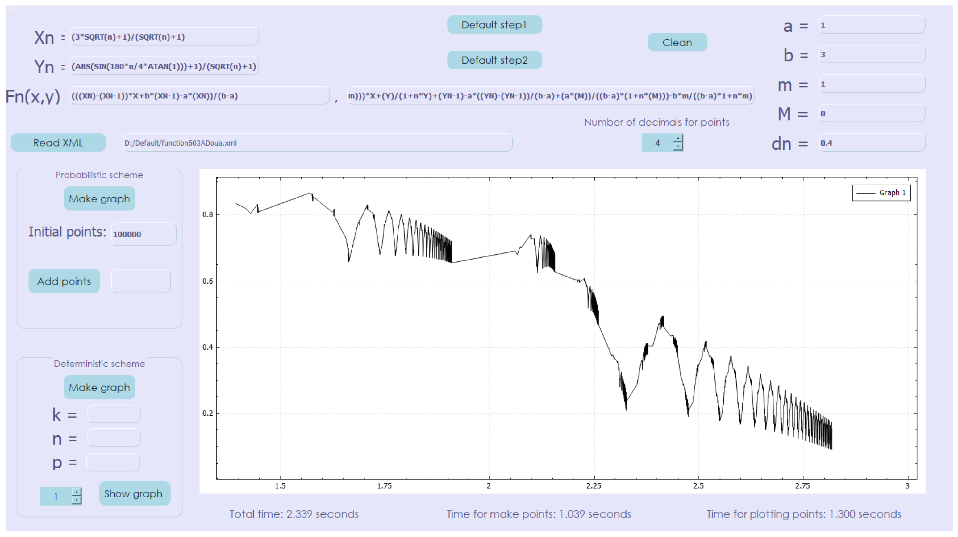
The probabilistic scheme (Algorithm 1), after 100,000 steps, leads us to the result shown in Figure 2.
Algorithm 1: The Probabilistic scheme.
  • Consider an empty set of points P R 2 and p a signifiant big signed positive integer.
  • Generate an arbitrary point ( x a , y a ) [ 0 , 1 ] × [ 0 , 1 ] .
  • Determine P { ( x a , y a ) } .
  • Generate a random signed integer 0 < k 100 .
  • Compute ( x a , y a ) = f k ( x a , y a ) .
  • Repeat steps 3, 4, 5 p times
  • Sort the elements of the set P in ascending order regarding the first component of the elements.
  • Plot the function passing through all the points of the set P .
Algorithm 2: The Deterministic Scheme
  • Consider k the number of the initial points, n the number of functions involved, p the number of steps and define an empty set of points P R 2 .
  • Generate randomly a set K 0 of k points in [ 0 , 1 ] × [ 0 , 1 ] .
  • Determine P K 0 .
  • Compute P = f 1 ( P ) f 2 ( P ) . . f n ( P )
  • Repeat step 4 for p times
  • Sort the elements of the set P in ascending order regarding the first component of the elements.
  • Plot the function passing through all the points of the set P .
The time spent to generate the points of the scheme was 1.039 s and the plotting time 1.3 s.
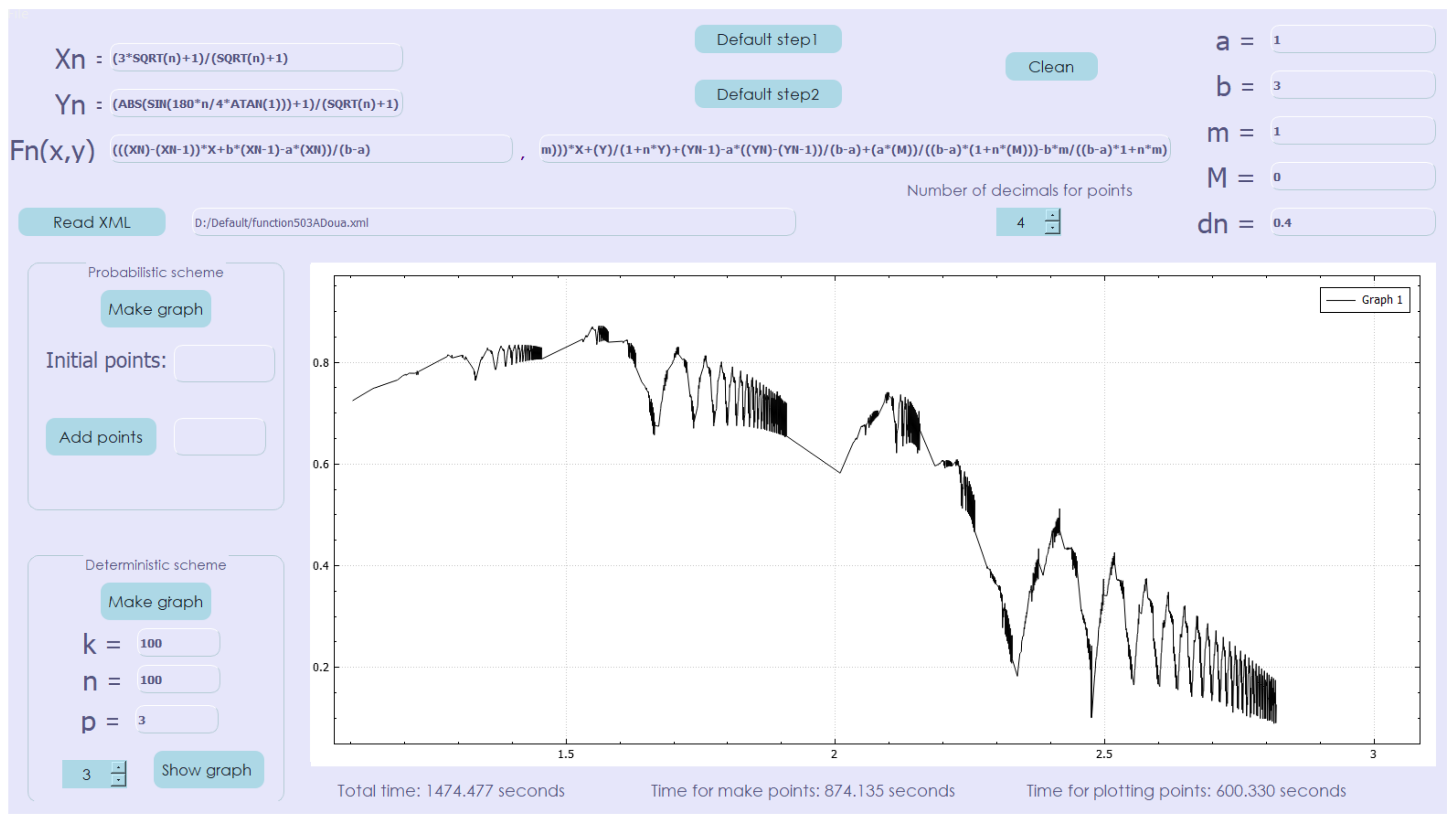
Using Algorithm 2, in the initial conditions of the probabilistic scheme, for the deterministic scheme taking k = 100 , n = 100 and p = 3 , we obtain the graph given in Figure 3. The scheme generated 100,000,000 points and the total duration of computing and plotting was 1474.477 s.
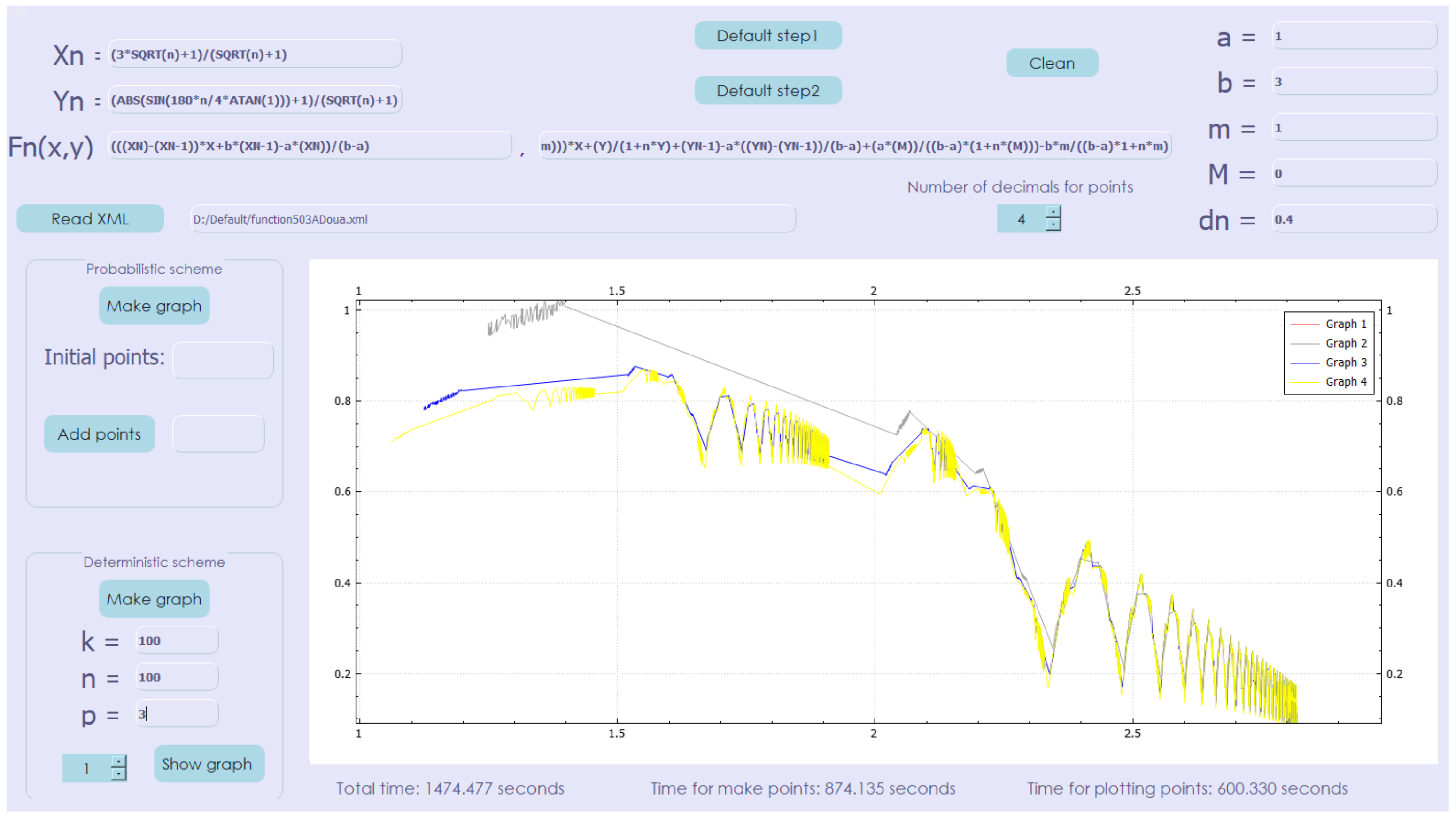
In Figure 4, a graph with the plotting of the interpolation function in every step of the algorithm is shown.

4.2. Countable Fractal Affine Interpolation Schemes

We made the study producing an approximation for the fractal countable affine interpolation scheme in the same two ways as for the non-affine case. Let us consider the positive, increasing, convergent sequence ( x n ) n N , the convergent sequence ( y n ) n N defined by
x n = 3 n + 1 n + 1 , y n = cos 180 · n π + 1 n + 1
and the affine sequence of functions ( f n ( x , y ) ) n N
f n ( x , y ) = x n x n 1 b a x + b x n 1 a x n b a , y n y n 1 b a d n M m b a x + d n y + b y n 1 a y n b a d n b m a M b a .
for all ( x , y ) [ x 0 , m ] × Y . The argument of the function cosinus we used when defining y n was imposed by the fact that the Mathematical Function Library demands us to work in radians.
For the desired approximation, we take the following subsets
X P = { x n | n 100 } , Y P = { y n | n 100 } , F P = { f n | n 100 }
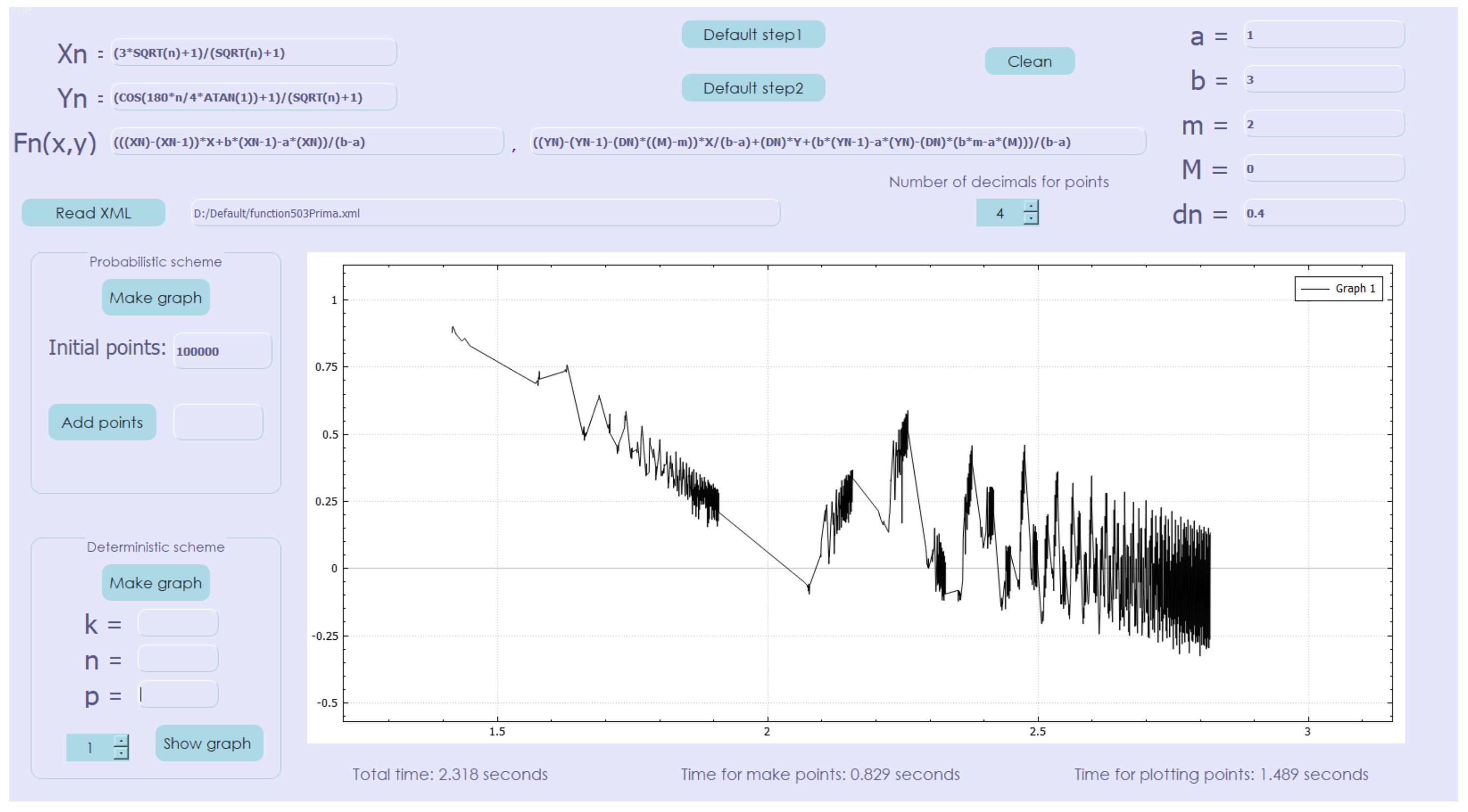
The probabilistic scheme (Algorithm 1), after 100,000 steps, leads us to the result shown in Figure 5.
The deterministic scheme produces, for k = 100 , n = 100 and p = 3 , the graph in Figure 6.
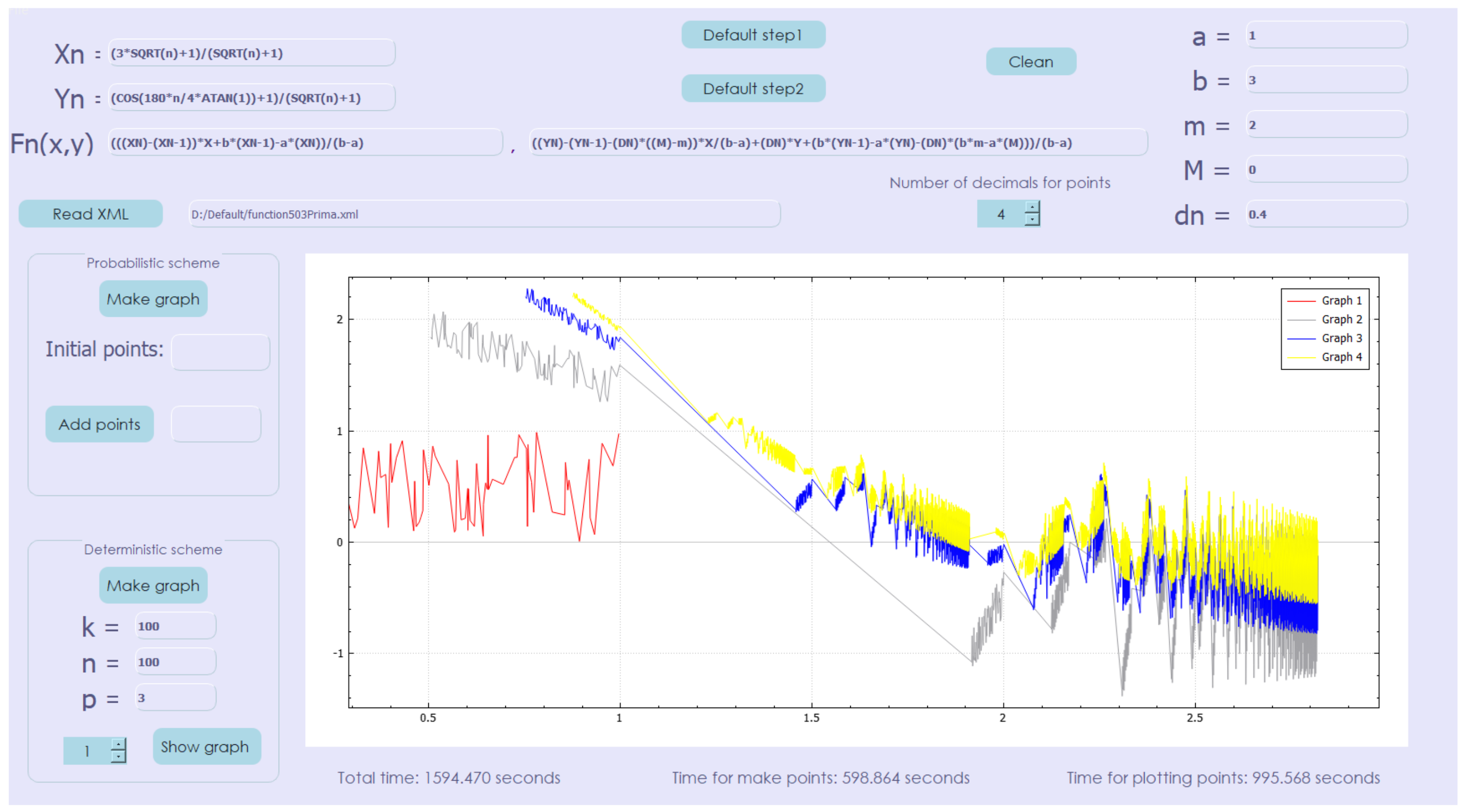
The time for obtaining the points in these conditions was 595.631 s and the time for plotting the function was 1594.470 s. The graph with the plotting of the interpolation function in every step of the algorithm is given in Figure 7.
The red graph is for the function given by the random generated 100 points. Graph 2 is the function for 10,000 thousand points (step for p = 1), graph 3 is for the function after step p = 2 (1,000,000 points) and the yellow graph is the final one—the same as in Figure 7.

5. Conclusions

The main conclusion of this study is that the algorithms presented give similar approximations of the FIFs for both schemes, affine and non-affine. For the probabilistic scheme (Algorithm 1), significant results are obtained for more than 10,000 steps and the time elapsed to plot the graph is less than two seconds. The deterministic scheme (Algorithm 2) permits the study of the variation of FIFs, step by step, but, in order to obtain significant results one must perform more than three steps. The time elapsed in this case is more than 1000 s. In the applications presented, both algorithms have an imposed number of steps.
Further studies are to be made in order to obtain a condition for stopping the algorithms if some conditions are fulfilled.
Besides the two algorithms, the computer application is a useful tool for plotting big sets of data generated by the iteration schemes described above through functions made in C++. It truly shows the capabilities of this programming language and it pushes it to the maximum using threading and modern programming techniques.

Author Contributions

Conceptualization: M.P.; introduction and preliminaries: C.M.P. and M.P.; methodology: M.P. and A.B.; visualization: A.B.; original draft preparation: M.P.; C.M.P. and A.B.; review, editing, validation, and formal analysis: M.P., C.M.P. and A.B. All authors have read and agreed to the published version of the manuscript.

Funding

This research received no external funding.

Institutional Review Board Statement

Not applicable.

Informed Consent Statement

Not applicable.

Data Availability Statement

Not applicable.

Acknowledgments

The authors want to express their gratitude for the reviewers. Their observations were very useful to improve the scientific value of the paper.

Conflicts of Interest

The authors declare no conflict of interest.

References

  1. Barnsley, M.F. Fractal functions and interpolation. Constr. Approx. 1986, 2, 303–329. [Google Scholar] [CrossRef]
  2. Barnsley, M. Fractals Everywhere; Academic Press: New York, NY, USA, 1988. [Google Scholar]
  3. Barnsley, M.F.; Elton, J.; Hardin, D.; Massopust, P. Hidden variable fractal interpolation functions. SIAM J. Math. Anal. 1989, 20, 1218–1242. [Google Scholar] [CrossRef]
  4. Mazel, D.S.; Hayes, M.H. Hidden-variable fractal interpolation of discrete sequences. In ICASSP 91: 1991 International Conference on Acoustics, Speech, and Signal Processing; IEEE Computer Society: Toronto, ON, Canada, 1991. [Google Scholar]
  5. Chand, A.K.B.; Kapoor, G.P. Hidden variable bivariate fractal interpolation surfaces. Fractals 2003, 11, 277–288. [Google Scholar] [CrossRef]
  6. Bouboulis, P.; Dalla, L. Hidden variable vector valued fractal interpolation functions. Fractals 2005, 13, 227–232. [Google Scholar] [CrossRef]
  7. Fernau, H. Infinite iterated function systems. Math. Nachrichten 1994, 170, 79–91. [Google Scholar] [CrossRef] [Green Version]
  8. Secelean, N. Countable Iterated Fuction Systems. Far East J. Dym. Syst. 2001, 3, 149–167. [Google Scholar]
  9. Secelean, N. Countable Iterated Function Systems; LAP Lambert Academic Publishing: Saarbrueken, Germany, 2013. [Google Scholar]
  10. Secelean, N. The fractal interpolation for countable systems of data. Univ. Beograd. Publ. Elektrotehn. Fak. Ser. Mat. 2003, 14, 11–19. [Google Scholar] [CrossRef]
  11. Secelean, N. Fractal countable interpolation scheme: Existence and affine invariance. Math. Rep. (Bucur.) 2011, 13, 75–87. [Google Scholar]
  12. Ri, S. A new idea to construct the fractal interpolation function. Indag. Math. 2018, 29, 962–971. [Google Scholar] [CrossRef]
  13. Kim, J.; Kim, H.; Mun, H. Nonlinear fractal interpolation curves with function vertical scaling factors. Indian J. Pure Appl. Math. 2020, 51, 483–499. [Google Scholar] [CrossRef]
  14. Ri, S.; Drakopoulos, V. How Are Fractal Interpolation Functions Related to Several Contractions? In Mathematical Theorems—Boundary Value Problems and Approximations; Alexeyeva, L., Ed.; IntechOpen: London, UK, 2020. [Google Scholar]
  15. Pacurar, C.M. A countable fractal interpolation scheme involving Rakotch contractions. arXiv 2021, arXiv:2102.09855. [Google Scholar]
  16. Dalla, L.; Drakopoulos, V.; Prodromou, M. On the box dimension for a class of non-affine fractal interpolation functions. Anal. Theory Appl. 2003, 19, 220–233. [Google Scholar] [CrossRef]
  17. De Amo, E.; Chiţescu, I.; Diaz Carrillo, M.; Secelean, N.A. A new approximation procedure for fractals. J. Comput. Appl. 2003, 151, 355–370. [Google Scholar] [CrossRef] [Green Version]
  18. Dubuc, S.; Elqortobi, A. Approximations of fractal sets. J. Comput. Appl. Math. 1990, 29, 79–89. [Google Scholar] [CrossRef] [Green Version]
  19. Chiţescu, I.; Miculescu, R. Approximation of fractals generated by Fredholm integral equations. J. Comput. Anal. Appl. 2009, 11, 286–293. [Google Scholar]
  20. Chiţescu, I.; Georgescu, H.; Miculescu, R. Approximation of infinite dimensional fractals generated by integral equations. J. Comput. Appl. Math. 2010, 234, 1417–1425. [Google Scholar] [CrossRef] [Green Version]
  21. Miculescu, R.; Mihail, A.; Urziceanu, S.-A. A new algorithm that generates the image of the attractor of a generalized iterated function system. Numer. Algorithms 2020, 83, 1399–1413. [Google Scholar] [CrossRef] [Green Version]
  22. Matkowski, J. Integrable solutions of functional equations. Dissertationes Math. 1975, 127, 68. [Google Scholar]
  23. Hutchinson, J. Fractals and self similarity. Indiana Univ. Math. J. 1981, 30, 713–747. [Google Scholar] [CrossRef]
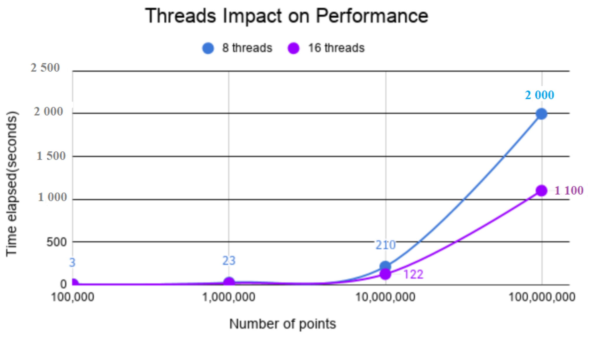
Figure 1. Threads impact on performance.
Mathematics 09 00767 g001
Figure 2. Non-affine probabilistic interpolation scheme (approximation with 100,000 points).
Mathematics 09 00767 g002
Figure 3. Non-affine deterministic interpolation scheme (approximation with 100,000,000 points).
Mathematics 09 00767 g003
Figure 4. Non-affine deterministic interpolation scheme (approximation with 100,000,000 points), plotting the graph of every step in the algorithm.
Mathematics 09 00767 g004
Figure 5. Affine probabilistic interpolation scheme (approximation with 100,000 points).
Mathematics 09 00767 g005
Figure 6. Affine deterministic interpolation scheme (approximation with 100,000,000 points).
Mathematics 09 00767 g006
Figure 7. Affine deterministic interpolation scheme (approximation with 100,000,000 points, step by step).
Mathematics 09 00767 g007
Publisher’s Note: MDPI stays neutral with regard to jurisdictional claims in published maps and institutional affiliations.