Abstract
In this work, we began to take forward kinematics of the Gough–Stewart (G-S) platform as an unconstrained optimization problem on the Lie group-structured manifold SE(3) instead of simply relaxing its intrinsic orthogonal constraint when algorithms are updated on six-dimensional local flat Euclidean space or adding extra unit norm constraint when orientation parts are parametrized by a unit quaternion. With this thought in mind, we construct two kinds of iterative problem-solving algorithms (Gauss–Newton (G-N) and Levenberg–Marquardt (L-M)) with mathematical tools from the Lie group and Lie algebra. Finally, a case study for a general G-S platform was carried out to compare these two kinds of algorithms on SE(3) with corresponding algorithms that updated on six-dimensional flat Euclidean space or seven-dimensional quaternion-based parametrization Euclidean space. Experiment results demonstrate that those algorithms on SE(3) behave better than others in convergence performance especially when the initial guess selection is near to branch solutions.
1. Introduction
The six degree-of-freedom Gough–Stewart (G-S) type motion platforms have been extensively employed to realize fully operational flight training simulation with high fidelity. This spatial G-S platform had six identical extensible active legs connected with an upper moving platform and a fixed lower platform using six upper passive joints and six lower passive joints. The forward kinematics of the G-S platform allows the platform to configure the pose (position and orientation) of end-effectors on the moving platform when the lengths of the six linear actuators are provided. However, the closed loop kinematic relations between the moving platform and the fixed base platform in 3-D space made forward kinematic problems a challenging issue among all kinematic research of parallel manipulators during the past few decades.
A significant amount of research has been focused on the forward kinematics of the G-S platform, which has lead us to understand the difficulty of this problem. Generally, there exist three main research directions to address the forward kinematics problem, which are the analytic method, numerical iterative method, and auxiliary-sensor-based method. The majority of early research focused on finding all possible closed-form direct solutions for different types of G-S platforms. Since Raghavan [1] and Ronga [2] firstly proved that there existed at most 40 distinct solutions in the complex domain for a general G-S platform, many researchers succeed in determining all 40 direct solutions using algebraic elimination, interval analysis, or numerical continuation methods, etc. Husty [3] obtained a 40-th degree univariate polynomial through complicated algebraic elimination based on a spatial kinematic mapping. For a symmetrical 6-6 G-S platform, the degree of polynomial was ultimately reduced to 14 by Huang [4]. Researcher Ji [5] focused on a special type 6-6 G-S platform in which both the fixed base platform and the moving platform are similar hexagons and only univariate quadratic equations are required to derive eight possible symmetry solutions by introducing a quaternion to represent the orientation matrix. As a general analytic form of direction solutions to forward kinematics of a general G-S platform was luxurious, some scholars resorted to the numerical root-finding method. Both Didrit [6] and Merlet [7] preferred to utilize the interval analysis method to numerically solve the forward kinematic problem for the general G-S platform. Wampler [8] implemented a polynomial continuation scheme to deal with this problem. Besides that, Dietmaier [9] proposed a numerical procedure to change the parameters of the G-S platform and ultimately obtained a particular asymmetry for the G-S platform, which possesses 40 real direct solutions.
As there exist multiple direct solutions, research attempting to solve the forward kinematic problem is further expected to determine a unique actual pose (position and orientation) of the G-S platform. Numerical iterative methods and auxiliary-sensor-based methods are two common schemes to pursue this goal. As the forward kinematic problem was easily boiled down to seeking six dimensional variables, satisfying six dimensional kinematic equations, Newton-type iterative algorithms were extensively put into use because of its simplicity and fast convergence speed [10,11]. However, it had been well known that the Newton-type algorithm usually converges to a particular solution near to initial guess value. Therefore, some variants of the Newton-type algorithm had been discussed to improve its performance in the following studies. Yang [12] modified the traditional Newton–Raphson algorithm using a monotonic descent operator to achieve global convergence regardless of the initial guess selection. Pratik [13] proposed a neural-network-based hybrid strategy that combined with the standard Newton–Raphson algorithm to yield better performance in dealing with uniqueness problem. Furthermore, Innocenti [14], Parenti-Castelli [15], and Chiu [16] suggested adding one or more redundant sensors to determine a unique real solution. Wang [17] designed a incremental iterative algorithm through a series of continuous small changes in leg length to derive a unique forward kinematic solution.
When iterative algorithms are employed to solve optimization that involves the SE(3) configure pose, the problem of which parametrization scheme is beneficial to design its updating framework must be addressed. As we all know, 3D+YPR and 3D+Quat are two common parametrization schemes, as explained in Reference [18]. In the 3D+YPR scheme, the iterative algorithm can be designed on flat Euclidean space with orthogonal constraints not taken into account. In the 3D+Quat scheme, a unit norm constraint equation is added while state vector is updated on enlarged Euclidean space . In this work, we address the forward kinematic as an unconstrained optimization problem on a Lie group-structured manifold SE(3). In algorithm construction, the updating direction and step size are computed on the associated tangent space with differential properties of the Lie group and Lie algebra. The result is then projected back on the manifold SE(3) to update the next configure pose. The advantage in the optimization on manifold SE(3) is that the exponential map that connects the Lie algebra and the Lie group naturally preserves the orthogonal constraint during each iteration. An experimental comparison is expected to show that the ways of simply updating the iteration on the local parameter space make the forward kinematic optimization algorithms more susceptible to being stuck in branch solutions.
The rest of this paper is organized as follows. In Section 2, some preliminary notations and terminology from the theory of Lie group and Lie algebra is reviewed. Section 3 is devoted to formulating the problem of forward kinematics for a general type G-S platform. Two kinds of iterative algorithms framework, the Gauss–Newton (G-N) and Levenberg–Marquardt (L-M) type algorithms are employed in algorithm construction with the mathematical tools from Lie group in Section 4. In Section 5, these two types of Lie group-based iterative algorithms are compared with traditional algorithms on Euclidean space as well as iterative algorithms using quaternion parametrization through a case study for a general G-S platform.
2. Preliminary Notations and Terminology
2.1. Lie Group and Lie Algebra
We assume that readers are familiar with basic mathematical concepts about group and manifold (see e.g., [19,20] and references therein). The configure pose of the G-S platform end-effector belongs to a special Euclidean group SE(3), which is a semi-direct product of with special orthogonal group SO(3). An element can be presented using a homogeneous transformation matrix as follows.
where is a orientation matrix, is a translational vector.
The inverse of g can be written in the following formulation,
Given a basis for matrix Lie algebra , any arbitrary element X, which is also called a “screw” matrix in the robot community, can be written in the following form,
where are listed as Equation (A1) in Appendix A.
Given a rigid body motion , its associated Lie algebra element shown as Equation (4) denotes a spatial screw matrix in an inertial frame. Meanwhile, Equation (5) denotes a screw matrix in body reference frame.
Accordingly, there exist two column vectors, spatial screw vector and body screw vector , which can be derived using following operation.
Here the vee operator is defined to extract screw coefficients from the screw matrix to form a column vector. Conversely, a wedge operator maps the screw vector back to the matrix Lie algebra , that is , .
2.2. Exponential Map
For each vector field X in tangent space at group identity e, there exists a smooth one-parameter subgroup of a Lie group G parametrized by a scalar . There also exists an exponential map defined as follows.
This is a unique homomorphism map from tangent space around group identity e to one-parameter subgroups of G. The exponential map is related with a one-parameter subgroup by at .
With these properties of the exponential map, we can define an integral curve of right invariant vector field passing through point at time zero as . Similarly, denotes an integral curve of left invariant vector field passing through at time zero.
As for special the Euclidean group SE(3), there exists an associated screw matrix as shown in Equation (3) at its tangent space . Then, motion around identity can be obtained by exponentiating these screw matrices. Here, the exponential map corresponds to matrix exponentiation, which has the closed-form Rodriguez formula as shown in Equation (A2) in the Appendix A. Examples for rotational screw vector and translational screw vector are expressed as follows,
2.3. Taylor Series Expansion of an Analytic Function on Lie Group
The Taylor series of a function on Euclidean space can be extended naturally to Lie group-structured non-Euclidean space. In the same way, there exists similar derivatives for group-valued function . Owing to the fact that there exist two invariant vector fields around , The Taylor series expansion around can be formulated in two ways. The following equation provides the right way.
As discussed in [21], the first and second-order term can be expressed in a different form. Analogously to directional derivative, the first-order term are completely equivalent to the following formulation,
Here, is called right Lie derivative of with respect to vector filed X. Since is a basis for Lie algebra , which can be shown as , then its associated differential operators will be denoted as . Thus, the right Lie derivative will be as follows,
Finally, the “right” Taylor series expansion around can be written to a second order in the following equation.
A “left” Taylor series expansion can also be derived in an analogous manner.
3. Problem Formulation of Forward Kinematics for G-S Platform
This section is devoted to formulating the forward kinematic problem of a general type G-S platform as a minimum optimization problem. The ultimate problem formulation depends on which parametrization scheme of configure pose is applied. Here, we take 3D + YPR scheme as an example, where position is in three-dimensional flat Euclidean space and orientation is parametrized by three angles in Yaw–Pitch–Roll order.
As for a general G-S platform, its geometric structure of a general G-S platform is depicted in the following Figure 1.
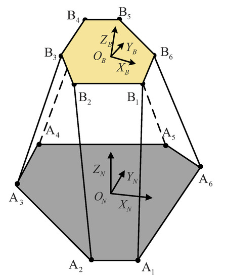
Figure 1.
Geometric structure of a general Gough–Stewart (G-S) platform.
It consists of one lower fixed platform and one upper moving platform connected through six identical extensible legs. Both two platforms are irregular hexagon structure with their six vertices located at one circumcircle.
In order to describe the relative configure pose between two platform, one coordinate frame is fixed at geometric center of lower fixed platform , another frame is fixed at geometric center of upper moving platform . Let denote the configure pose (position and orientation) of geometric center of upper moving platform represented in lower fixed frame .
where orientation matrix is defined by successive rotation in Z-Y-X order.
Let denote the position vector of the lower joint center of i-th leg in frame , and let denote the position vector of upper joint center of i-th leg in frame .
The inverse kinematic function of the G-S platform defined as a six dimensional real-valued function describes a kinematic mapping from configure pose T of upper moving platform to its six leg lengths .... If T is locally parametrized by 3D+YPR generalized coordinate variable ; thus, the ultimate inverse kinematic function is defined as follows.
The forward kinematic problem of the G-S platform is formulated as a minimum optimization problem related with kinematic mapping residual error . Each component of is defined as follows.
where are six scalars for current leg length.
Let denote the objective function in the following formulation.
As shown in Figure 2, local parametrization of objective function around configure point T is described as follows,
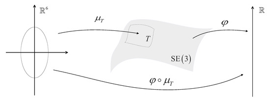
Figure 2.
is a local parametrization of function around configure pose T expressed in local parameter space .
Finally, forward kinematic problem of the G-S platform can be formulated as a minimum optimization problem as follows.
where domain denotes accessible workspace configure pose of the G-S platform.
4. Iterative Algorithms on SE(3)
As discussed in the introduction section, it will take considerable efforts before we can arrive at an analytical solution to solve the forward kinematic problem in Equation (20). In consideration of this difficulty, many numerical iteration algorithms, e.g., G-N and L-M, have been extensively applied in practical engineering projects.
In order to minimize the quadratic sum of kinematic residual error , the numerically iterative algorithm is updated iteratively by means of a small increment until convergence or the max number of iteration is reached. It should be noticed that all these numerical iteration schemes are originally designed to work on flat Euclidean space, i.e., . If the update process was designed on generalized coordinates according to Equation (16), there exists a gimbal lock problem as well as three Euler angles that may reach out of their valid ranges. In this section, we begin to build up two elegant iterative algorithms on the Lie group-structured manifold SE(3) with differential properties from theory of the Lie group and Lie algebra.
The core issue in the Newton-type algorithm construction process is to determine the small increments at each step through solving incremental normal equations related with the first-order Taylor series expansion. According to Equation (13), the six-dimensional inverse kinematic residual error function can be approximated in the neighborhood of with first-order “right” Taylor series expansion as follows.
As for computing the first order term, right Lie derivative of six-dimensional vector-valued residual function was defined as . Each Lie derivative with respect to body screw matrix can be derived using the following formulation.
where tilde on and means a extension by adding an extra element 1, that is and .
Similarly, a left Lie derivative with respect to spatial screw matrix can be used to approximate in “left” Taylor series expansion.
All these six right Lie derivatives can be formed into a Jacobian matrix, which is named right Lie derivative matrix with respect to body screw matrix as follows.
Then Equation (21) can be arranged in form of body screw vector as follows.
Thus we can obtain body screw error by assuming . This means that the updating direction in Lie algebra vector space at time step can be given as follows.
After its updating direction has been chosen, a step factor that satisfies the following monotonic descent rule is dedicated to constraint step size at time so as to avoid divergence during iterative process. If initial setting of step factor cannot meet this rule, then multiply by itself until the descent rule is met.
Once a descent step size has been determined, the next configure pose can be updated by mapping selected descent screw error in Lie algebra to Lie group using the exponential map.
In the end, a Lie group-based G-N algorithm for the forward kinematics of the G-S platform can be constructed as the Algorithm A1 in the Appendix B. Figure 3 provides an intuitive explanation of this algorithm.
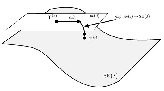
Figure 3.
Updating process of G-N type algorithm on Lie group SE(3).
However, it is well known that G-N type algorithms depend heavily on good local linearization around selected expansion points. As to this issue, L-M type algorithms behave better in adjusting to a descent direction within an appropriate dynamically tuned trust region. An L-M type iterative algorithm under the framework of the Lie group is shown in Algorithm A2 in the Appendix B.
5. Implementation of Algorithms and Discussions
In this section, we first compare the aforementioned Lie group-based G-N type iterative algorithm (GN-SE(3)) with corresponding G-N type algorithms (GN-Quat and GN-). Then, it is followed with three L-M type algorithms (LM-SE(3), LM-Quat, and LM-). A general type G-S platform is leveraged to test the performance of these algorithms. The following Table 1 provides those lower joint coordinate vectors on fixed platform and upper joint coordinate vectors on moving platform frame as referred in [22].

Table 1.
Coordinate vectors of the G-S platform’s upper and lower joints with respect to their own coordinate frame.
Take a group of current leg lengths as our destination , which corresponds to the true value of platform pose . Figure 4a provides true state of G-S platform in 3D Cartesian coordinate frame.
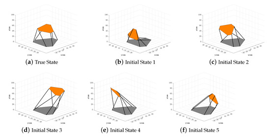
Figure 4.
True state and five initial guess states of the G-S platform.
Due to the existence of multiple solutions for the G-S platform, we can easily find out another two branch solutions and that correspond to the same lengths group . Although the two branch solutions and are represented with different Euler angles, their orientation parts actually correspond to the same orientation matrix. Therefore, both branch solutions and should be regarded as one configure pose as follows. The following Figure 5 gives its platform state in 3D Cartesian space.
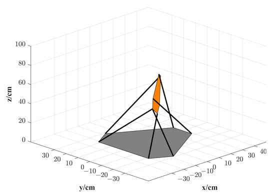
Figure 5.
Platform state corresponding to branch solutions and .
In algorithm initialization phase, five configure poses as shown in Table 2 are provided as initial guess states to testify to three kinds of G-N type forward kinematic algorithms. All these initial states are chosen to be far away from the true value . The choice of these five configure poses are based on the performance that G-N and L-M algorithms on (GN- and LM-) act at these initial guess states. State 1, state 2, and state 4 represent a group of initial guess values that GN- and LM- deteriorated quickly, while state 3 and state 5 represent the opposite type of initial guess value, these two algorithms converged to the true value normally.
Table 2.
Five initial configure poses of the G-S platform and performance comparison of G-N type algorithms.
The other algorithms that were constructed on quaternion-based Euclidean space and SE(3) are expected to improve the convergence performance when starting from state 1, state 2, and state 4 because both of them have kept the orthogonal constraint at each iteration process. Meanwhile, state 3 and state 5 are necessary moderate choices to verify the reliability of the other two algorithms. In order to evaluate the influence of the step factor on algorithm performance, the step factor is selected from 0.50 to 0.99 with an equal interval of 0.01. The reason to choose a relatively large value for the step factor is to make sure at least half of the derived updating direction could be exploited at each iteration. All tested G-N type algorithms share the same accuracy threshold (, , ), and max iteration time to end their iteration. Figure 4b–f corresponds to these five initial guess states of the G-S platform, respectively.
In this experiment, two criteria were employed to evaluate algorithm performance, one is the range of step factor that converges to true value , the other is convergence speed. The algorithm performance reflects significant difference among these five initial states. Their performance difference comparisons are shown in Figure 6 and Figure 7, which take step factor and iteration time as their coordinate axes. Let the positive direction of longitudinal axis indicate the iteration time that an algorithm reaches final true value within given accuracy threshold while negative direction indicates the iteration time that it takes to converge to other branch solutions. This comparison analyst yields the following conclusions.
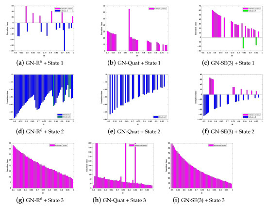
Figure 6.
G-N algorithm performance comparison for initial guess state 1, state 2, and state 3.
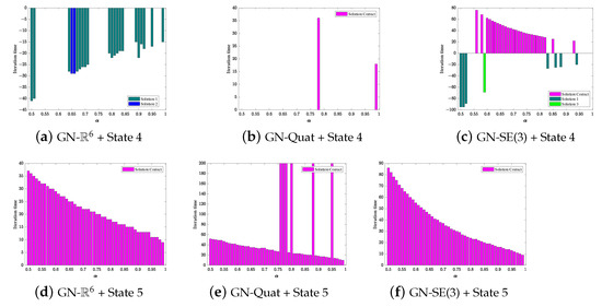
Figure 7.
G-N type algorithm performance comparison for initial guess state 4 and state 5.
- For GN-, it achieves fast convergence when it starts from state 2, state 3, and state 5. However, it is more likely to reach one branch solution when state 2 is selected. For state 4, the algorithm is inclined to another branch solution within some isolated range. As to state 1, due to its divergence under the large range of the step factor, it means that state 1 is not an appropriate choice for the GN- initial guess value.
- For GN-Quat, it ends up with the true value among some isolated range of step factor when starting from state 1. For state 2, it always converges to . For state 3 and state 5, although it achieves convergence to the true value , but it could possibly behave worse if the convergence speed is slowed down at some specific larger step factors. The state 4 is definitely no longer a suitable choice for GN-Quat algorithm initialization.
- For GN-SE(3), when it starts from state 3 and state 5, it always converges to the true value and the larger step factor would be helpful to reduce iteration time. When state 1 is provided as the initial guess state, it converges to the true value with a probability of more than fifty percent. For state 4, it converges to the true value with a consecutive range from 0.60 to 0.84.
In the second comparison experiment, these five configure poses were provided as input to L-M type algorithms (LM-, LM-Quat and LM-SE(3)). Their performance comparison with respect to the damping ratio is given in Table 3. The logarithmic of the damping ratio that was taken as horizontal coordinate is assigned to a range between −9 and −3.12 with an equal interval of 0.12. Its iteration time is taken as its longitudinal coordinate. All these tested L-M type algorithms share the same accuracy threshold (, ) and max iteration time to terminate their iteration.
Table 3.
Five initial configure poses of the G-S platform and performance comparison for L-M type algorithms.
As seen in Table 3 and Figure 8, if state 3 is employed for algorithm initialization, all three kinds of L-M type algorithms converge to the true value at an acceptable speed in the whole range of the damping ratio . However, there exists obvious performance differences between these L-M type algorithms when the four other states are used to initialize these algorithms. Their performance comparisons are arranged in Figure 8 and Figure 9. From these comparisons, we can draw the following conclusions,
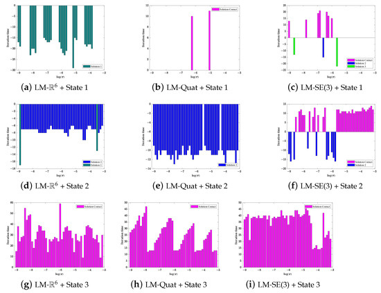
Figure 8.
L-M type algorithm performance comparison for initial guess state 1, state 2, and state 3.
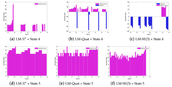
Figure 9.
L-M algorithm performance comparison for initial guess state 4 and state 5.
- For LM-, when its is initialized from state 5, it achieves fast convergence toward true value in the whole range of damping factor. However, it is more likely to converge to branch solution when state 2 is employed. If state 4 is taken into consideration, it reaches the true value within some isolated regions for damping factor selection. As to state 1, it has a higher chance to converge to the branch solution within some isolated regions.
- For LM-Quat, it would converge to the true value when it starts form state 5. From state 2, it also achieves almost total convergence towards branch solution . For state 1, it is definitely not suitable for initialization as it cannot converge to any solution within the whole selection range. Finally, when the algorithm initialized from state 4, it can achieve some convergence to the true value within some isolated regions for damping factor .
- For LM-SE(3), it can converge to the true value with almost the whole range of damping factor selection except some large values. For state 2, it behaved better in convergence to the true value when the logarithm value of the damping factor is selected from −5.5 to −3.12. For state 1 and state 4, its convergence probability towards the true value is quite small, which means that the two states cannot be appropriate for LM-SE(3) algorithm initialization.
Finally, we consider two evaluation indicators for the initial guess state selection, convergence probability toward the true value and consecutive region for influence factors’ selection. For GN type algorithms, state 1, state 4, and state 5 are totally or conditionally suitable for LM-SE(3). State 5 is the only suitable initial guess state for GN- and conditionally acceptable for GN-Quat. For LM type algorithms, state 5 is totally suitable initial guess state choice for all three algorithms. Meanwhile, state 2 is conditionally acceptable for LM-SE(3) algorithm.
In summary, we can arrive at some conclusions through the above comparative analysis. Firstly, the iterative algorithms constructed on SE(3) would leave more space for initial guess state selection in the workspace of the G-S platform. Secondly, the algorithm on SE(3) has few chances to be stuck in other branch solutions even though the initial guess value is near to the branch solution.
6. Conclusions
In this paper, we discussed how to construct G-N and L-M type iterative algorithms (GN-SE(3) and LM-SE(3)) to solve the forward kinematics problem of a G-S platform with mathematical tools from the Lie group. The key part of the Lie group-based iterative algorithm was to determine an updating direction in Lie algebra and was then projected back to the Lie group SE(3) with exponential map, which differentiates the algorithm from traditional iterative algorithms based on locally Euclidean space or quaternion-based parametrization space . Five different initial configure poses of a general G-S platform were used to compare Lie group-based algorithms (GN-SE(3) and LM-SE(3)) with two other kinds of iterative algorithms. Experiment results demonstrated that Lie group-based iterative algorithms behave better in converging to the true solution while the two other algorithms leave more chance in converging to another branch solutions. In the future, more work is needed to study how geometric parameters of the G-S platform can influence the choice of the iterative forward kinematic algorithm.
Author Contributions
Conceptualization, B.X.; investigation, B.X.; methodology, B.X.; project administration, S.D.; resources, B.X.; software, F.L.; supervision, S.D.; validation, B.X.; visualization, B.X.; writing—original draft, B.X.; writing—review and editing, S.D. and F.L. All authors have read and agreed to the published version of the manuscript.
Funding
This work is supported by the National Key Research and Development Plan of China (No. 2018AAA0102902).
Institutional Review Board Statement
Not applicable.
Informed Consent Statement
Not applicable.
Data Availability Statement
Not applicable.
Conflicts of Interest
The authors declare no conflict of interest.
Appendix A
Appendix A.1.
The following are six basis components for matrix Lie algebra .
Appendix A.2.
The Rodriguez formula for screw matrix S in is as follows,
where .
Appendix B
The G-N algorithm that constructed on Lie group-structured manifold SE(3) are shown as follows. Here, denotes the updating direction in Lie algebra vector space during each iteration.
| Algorithm A1 G-N Type Algorithm on SE(3) for solving the forward kinematics problem of a G-S platform. |
| Input: Coordinate vectors of upper and lower joints with respect to their own coordinate frames: ; ; Current leg lengths: ; Initial Configuration pose: ; Accuracy threshold: , , ; Max iteration time . |
| Output: Final configuration pose: . |
| 1: , ; |
| 2: , ; |
| 3: found |
| 4: while (not found) and do |
| 5: ; |
| 6: Solve normal equation: ; |
| 7: if then |
| 8: ; |
| 9: |
| 10: ; |
| 11: while (accept or ) do |
| 12: && ; |
| 13: ; |
| 14: end while |
| 15: if then |
| 16: ; //No appropriate descent step |
| 17: else |
| 18: ; //Update configuration pose |
| 19: , ; |
| 20: ; |
| 21: end if |
| 22: end if |
| 23: end while |
| 24: return Final configure pose . |
Likewise, the L-M type algorithm on SE(3) is constructed as follows. Here, denotes the updating direction in Lie algebra vector space during each iteration process.
| Algorithm A2 L-M Type Algorithm on SE(3) for solving the forward kinematics problem of G-S platform. |
| Input: Coordinate vectors of upper and lower joints with respect to their own coordinate frames: ; ; Current leg lengths: ; Initial Configuration pose: ; Accuracy threshold: , ; Max iteration time . |
| Output: Final configuration pose: . |
| 1: , ; |
| 2: , ; |
| 3: , ; |
| 4: while and do |
| 5: .; |
| 6: Solve: ; |
| 7: if then |
| 8: ; |
| 9: else |
| 10: ; |
| 11: ; |
| 12: if then |
| 13: ; |
| 14: , ; |
| 15: ; |
| 16: , ; |
| 17: else |
| 18: , ; |
| 19: end if |
| 20: end if |
| 21: end while |
| 22: return Final configure pose . |
References
- Raghavan, M. The Stewart platform of general geometry has 40 configurations. J. Mech. Des. 1993, 115, 277–282. [Google Scholar] [CrossRef]
- Ronga, F.; Vust, T. Stewart platforms without computer. In Proceedings of the Conference Real Analytic and Algebraic Geometry, Trento, Italy, 21–25 September 1992; De Gruyter: Berlin, Germany, 1995; pp. 197–212. [Google Scholar]
- Husty, M.L. An algorithm for solving the direct kinematics of general Stewart-Gough platforms. Mech. Mach. Theory 1996, 31, 365–379. [Google Scholar] [CrossRef]
- Huang, X.; Liao, Q.; Wei, S. Closed-form forward kinematics for a symmetrical 6-6 Stewart platform using algebraic elimination. Mech. Mach. Theory 2010, 45, 327–334. [Google Scholar] [CrossRef]
- Ji, P.; Wu, H. A closed-form forward kinematics solution for the 6-6/sup p/Stewart platform. IEEE Trans. Robot. Autom. 2001, 17, 522–526. [Google Scholar]
- Didrit, O.; Petitot, M.; Walter, E. Guaranteed solution of direct kinematic problems for general configurations of parallel manipulators. IEEE Trans. Robot. Autom. 1998, 14, 259–266. [Google Scholar] [CrossRef]
- Merlet, J.P. Solving the forward kinematics of a Gough-type parallel manipulator with interval analysis. Int. J. Robot. Res. 2004, 23, 221–235. [Google Scholar] [CrossRef]
- Wampler, C.W. Forward displacement analysis of general six-in-parallel SPS (Stewart) platform manipulators using soma coordinates. Mech. Mach. Theory 1996, 31, 331–337. [Google Scholar] [CrossRef]
- Dietmaier, P. The Stewart-Gough platform of general geometry can have 40 real postures. In Advances in Robot Kinematics: Analysis and Control; Springer: Berlin/Heidelberg, Germany, 1998; pp. 7–16. [Google Scholar]
- Dieudonne, J.E.; Parrish, R.V.; Bardusch, R.E. An Actuator Extension Transformation for a Motion Simulator and an Inverse Transformation Applying Newton-Raphson’s Method; National Aeronautics and Space Administration: Columbia, WA, USA, 1972.
- Koekebakker, S. Coordinate reconstruction in model based control of a Stewart platform. IFAC Proc. Vol. 1998, 31, 103–108. [Google Scholar] [CrossRef]
- Yang, C.; He, J.; Han, J.; Liu, X. Real-time state estimation for spatial six-degree-of-freedom linearly actuated parallel robots. Mechatronics 2009, 19, 1026–1033. [Google Scholar] [CrossRef]
- Parikh, P.J.; Lam, S.S. A hybrid strategy to solve the forward kinematics problem in parallel manipulators. IEEE Trans. Robot. 2005, 21, 18–25. [Google Scholar] [CrossRef]
- Innocenti, C. Closed-form determination of the location of a rigid body by seven in-parallel linear transducers. J. Mech. Des. 1998, 120, 293–298. [Google Scholar] [CrossRef]
- Parenti-Castelli, V.; Di Gregorio, R. A new algorithm based on two extra-sensors for real-time computation of the actual configuration of the generalized stewart-gough manipulator. J. Mech. Des. 2000, 122, 294–298. [Google Scholar] [CrossRef]
- Chiu, Y.J.; Perng, M.H. Forward kinematics of a general fully parallel manipulator with auxiliary sensors. Int. J. Robot. Res. 2001, 20, 401–414. [Google Scholar] [CrossRef]
- Wang, Y. A direct numerical solution to forward kinematics of general Stewart-Gough platforms. Robotica 2007, 25, 121. [Google Scholar] [CrossRef]
- Blanco, J.L. A tutorial on se (3) transformation parameterizations and on-manifold optimization. Univ. Malaga Tech. Rep. 2010, 3, 6. [Google Scholar]
- Kamedulski, B. Product property of equivariant degree under the action of a compact abelian Lie group. In Bulletin of the Brazilian Mathematical Society; Springer Science & Business Media: Berlin/Heidelberg, Germany, 2020; pp. 1–13. [Google Scholar]
- Fermanian-Kammerer, C.; Fischer, V. Defect measures on graded lie groups. In Annali della Scuola Normale Superiore di Pisa—Classe di Scienze 21 Special Issue; Scoula Normale Superiore: Pisa, Italy, 2020; pp. 207–291. [Google Scholar]
- Chirikjian, G.S. Stochastic Models, Information Theory, and Lie Groups, Volume 2: Analytic Methods and Modern Applications; Springer Science & Business Media: Berlin/Heidelberg, Germany, 2011; Volume 2. [Google Scholar]
- Cardona, M. Kinematics and Jacobian analysis of a 6UPS Stewart-Gough platform. In Proceedings of the 2016 IEEE 36th Central American and Panama Convention (CONCAPAN XXXVI), San Jose, Costa Rica, 9–11 November 2016; pp. 1–6. [Google Scholar]
Publisher’s Note: MDPI stays neutral with regard to jurisdictional claims in published maps and institutional affiliations. |
© 2021 by the authors. Licensee MDPI, Basel, Switzerland. This article is an open access article distributed under the terms and conditions of the Creative Commons Attribution (CC BY) license (https://creativecommons.org/licenses/by/4.0/).