Article

Unified CACSD Toolbox for Hybrid Simulation and Robust Controller Synthesis with Applications in DC-to-DC Power Converter Control

Department of Automation, Technical University of Cluj-Napoca, Str. G. Bariţiu nr. 26-28, 400027 Cluj-Napoca, Romania
*
Authors to whom correspondence should be addressed.
These authors contributed equally to this work.
Mathematics 2021, 9(7), 731; https://doi.org/10.3390/math9070731
Submission received: 28 February 2021 / Revised: 20 March 2021 / Accepted: 23 March 2021 / Published: 28 March 2021
(This article belongs to the Special Issue Applications of Mathematical Models in Engineering)

Abstract

:
The current article presents the design, implementation, validation, and use of a Computer-Aided Control System Design (CACSD) toolbox for nonlinear and hybrid system uncertainty modeling, simulation, and control using μ synthesis. Remarkable features include generalization of classical system interconnection operations to nonlinear and hybrid systems, automatic computation of equilibrium points for nonlinear systems, and optimization of least conservative uncertainty bounds, with direct applicability for μ synthesis. A unified approach is presented for the step-down (buck), step-up (boost), and single-ended primary-inductor (SEPIC) converters to showcase the use and flexibility of the toolbox. Robust controllers were computed by minimization of the H norm of the augmented performance systems, encompassing a wide range of uncertainty types, and have been designed using the well-known mixed-sensitivity closed loop shaping μ synthesis method.

1. Introduction

Robust Control represents a massive point of interest when it comes to Control Theory, which has been heavily studied over the past decades. However, albeit Robust Control brings many benefits, it is still an open field in research which gathers increasingly more approaches over time. Basically, the goal of a robust controller is to accomplish a specified set of performances for bounded model uncertainties which can occur in practice due to various reasons. In other words, closed loop stability and performance are maintained even for model parameter variations and unmodeled dynamics alike.
Over the years, multiple and various approaches for designing robust controllers have been presented, some of them being implemented into dedicated toolboxes, such as MATLAB’s Robust Control Toolbox [1]. This toolbox gathers the most efficient ones based on H 2 , H , and μ synthesis methods, and it is often considered a reference in research. However, while using these types of toolboxes leads to controllers which are optimal for their prescribed criterion, they are not necessarily best in terms of conventional performances. Additionally, of great use for defining and optimizing difficult robust control problems is the Global Optimization Toolbox from in [2], providing ready-to-use solvers using various state-of-the-art algorithms, such as Particle Swarm Optimization (PSO) and Genetic Algorithms (GA). An important work in this direction, for computing optimal weighting functions for the generalized plant model, is presented in [3].
Even though there is a large variety of CACSD toolboxes in the field, their number is still expanding due to the necessity of overcoming drawbacks that the already existing ones have. At this point, the purpose of new toolboxes is not only to determine robust controllers for a specific process class, but to use a unified approach that would make them work for more types of systems, even multiple interconnected systems, in various configurations. User experience is also more accentuated, which is why some of them incorporate graphical user interfaces (GUIs), for improved usability.
An example is Multivar, which is a MATLAB-based application used for multiple-input and multiple-output (MIMO) control design, presented in [4]. This toolbox supports two working modes. It allows the user to work both in function and GUI mode (which represents a configuration wizard for determining the controller). Multivar can be used for LTI systems with or without time delay and it allows creating a model; converting, approximating, and analyzing it; input–output pairing and decoupling; and controller design and evaluation. Besides this, the user is able to export the control design and compare it with other saved designs. Another GUI-based robust controller design tool, which was created in LabVIEW, is presented in [5], based on the H loop shaping method. However, the goal was to provide a simple, user-friendly interface to make it easier to use, especially for educational purposes. Therefore, as mentioned by the authors, it does not provide the same flexibility as other design tools on the market.
LCToolbox, as presented in [6], is another MATLAB software package which is used for robust controller design. One of the advantages of using this toolbox instead of classic MATLAB routines is the fact that it gathers all necessary steps for controller design in one place, while cutting the need of preprocessing steps such as separate construction of the plant, and postprocessing steps, such as closed loop simulation. LCToolbox can be used for both linear time-invariant (LTI) and linear parameter-varying (LPV) models, and it also incorporates system identification methods. The controller is obtained by using the H loop shaping method. Other H -based CACSD toolboxes have been presented over the past years. One example is represented in [7], which is based on linearizing or convexifying the conventional non-convex constraints on the classical robustness margins of H constraints. The controller parameters are then computed by using an optimization solver. This toolbox was created for MATLAB, and some of its main features are represented by the large variety of control problems in which it could be used, such as multi-model systems; the toolbox is designed to work with the output data of MATLAB’s System Identification Toolbox [8]. The output of the toolbox is represented by a PID controller, which can be easily implemented. Another example of a H -based CACSD toolbox is shown in [9], in which the main advantage is the reduced conservatism of almost all types of model uncertainties which are defined.
Controller order is an important factor when implementing it on real systems. Therefore, this might be an issue in some cases. However, methods that are determining a fixed structure controller are already presented, such as in [10], which is based on the H 2 controller design method, but can be cumbersome to compute. In order to deal with the high order controller problem, other toolboxes include controller simplification steps to avoid the necessity of postprocessing, as presented in [11].
Currently acknowledged problems in this domain regard closed loop simulation, where performance validation is generally treated ad hoc, from one control problem to another. Another difficulty encountered is when the test cases were done only on the linearized system for which the controller is designed, without checking if the initially proposed performance values are additionally verified for the nonlinear plant model, and, also, uncertainty modeling is a very cumbersome operation. The purpose of the paper is to provide means for treating the previously stated problems in a unified manner, such as implementing automated testing, performance validation, and report generation.
In this current iteration of the toolbox, robust controllers were designed using the well-established routines from in [1]. The interface is scalable and the control logic and validation can be replaced with other user-defined methods, or the current robust control approach can be replaced with open source alternatives for the H 2 and H optimization problems, such as presented in the thesis [12], with the possibility to refine the necessary solutions of the Algebraic Riccati Equations (AREs) using the algorithms from [13], while for the μ synthesis problem, the thesis [14] provides a flexible, open-source implementation using linear matrix inequalities (LMIs). A clear advantage over the ARE approach is that LMIs are capable of solving singular and close to singular problems. Alternatively, a mixed H 2 / H approach for stabilization and optimization using fixed-order controllers can be found in [15]. As such, the current iteration of the proposed toolbox is MATLAB-dependent for certain key functionalities, especially with regards to numerical simulation, robust control, and optimization, although the exposed ideas and mathematical framework can be directly implemented in other software environments, such as Python, Scilab, or LabVIEW.
The remainder of the paper is structured in the following manner. Section 2 describes the software structure and features of the proposed toolbox; Section 3 describes a proposed end-to-end workflow exemplified using modeling, control, validation, and simulation of several DC-to-DC converter topologies; and Section 4 illustrates comparative discussions, proposed improvements, and completions for future work and conclusions.

2. Toolbox Structure and Functionalities

The proposed toolbox has been designed with the target of end-to-end design and implementation of closed loop control systems, starting from the definition of the uncertainty set of plants to be controlled, their required operating point, along with control performance specifications and controller synthesis, and ending with the controller validation for the initial desired plant set.

2.1. Toolbox Features

Proposed features and advantages over existing toolboxes available in the literature:
  • specify finite-dimensional dynamical systems with the general framework from Equation (1) to be used with the MATLAB ode framework; ability to interconnect such systems in series, parallel, and linear-fractional transformations; this functionality is described in Section 2.2.1 and Section 2.2.2;
  • specify hybrid dynamical systems in the framework from in [16] as in Equation (4), with the ability to interconnect such systems in series, parallel, and linear-fractional transformations, upper and lower; this feature is described in Section 2.2.3;
  • automatically compute equilibrium points numerically, with the possibility to impose certain states, inputs, and/or outputs, while the remaining ones are deduced through numerical optimization; this feature is presented in Section 2.4;
  • automatically compute the uncertainty model as requested alongside a nominal plant: additive, inverse additive, input and output multiplicative, etc. using a global optimization algorithm, such as particle swarm optimization, to be directly used as necessary for robust synthesis methods; removes the burden for the control engineer to manually do this process for each plant; this feature is presented in Section 2.5;
  • flexible and scalable, all features are implemented through MATLAB code and does not need the use of Simulink, which can become cumbersome when treating families of plants and not a single, specific, plant at a time; also, to account for the operating point in the case of linearized, nonlinear, and hybrid systems, alike, the same interface for Model-in-the-Loop simulation is provided in the toolbox, as shown in Section 2.2 and Section 2.3;
  • besides the automatic validation of the frequency response for the desired operating point of the linearized plant family, the toolbox runs tests accounting for the uncertainty behavior of the desired nonlinear plant, not only on the linearization which the controller has been designed for. Every specification imposed in the designed phase will be automatically tested for the entire nonlinear system family, as illustrated in the case studies from Section 3.

2.2. Systems Specification

The scope of software classes implemented and described in this section aims to provide a flexible framework for simulation by using the ordinary-differential equation ode solver exclusively, with the low-level requirement of integrating a differential state equation. As such, exogenous signals would be reference signals and disturbances, known a priori in a simulation context. The intrinsic signals, i.e., commands and corresponding measurements, are passed to their corresponding subsystems by means of ode. Figure 1 encompasses an overview of the toolbox classes described in Section 2.2, Section 2.3 and Section 2.4. When the relationship between two classes is of type inheritance, the inherited class will not redundantly recall all previous properties and methods from the base class in the diagram, unless they overload the methods and is explicitly noted.

2.2.1. Nonlinear Systems

For the purpose of this paper, we will focus on finite-dimensional systems: deterministic and stochastic. The so-called explicit or standard system form is obtained by writing the plant model in the following canonical form, using a set of differential equations and a set of output equations:
{ (1a) x ˙ ( t ) = F x ( t ) , u ( t ) , t ; (1b) y ( t ) = h x ( t ) , u ( t ) , t ,
with the vector maps F and h being Lipschitz functions. The input signal u ( t ) has dimension m, state signal x ( t ) with dimension n, and output signal y ( t ) with dimension p, with t 0 . The initial conditions of the system are x ( 0 ) = x 0 R n .
Dynamical systems of the form (1) are implemented in class System. This will be the baseline interface for all systems the toolbox works with. Its most important methods are sim, findEqPoint, and linearize, which will be briefly described. The method sim simulates the dynamical system described by Equation (1a) from the initial condition x0, using the exogenous signal u(t), which is a predetermined anonymous function with at least the input argument time. tfin can be a scalar time value representing the final simulation time, a simulation interval, or a vector of predetermined time values. The solver options and type are based on MATLAB’s ode framework options and are sent directly to it. The solver type can be selected from any of the supported functions: ode113, ode15s, ode15i, ode23, ode23t, ode23s, ode23tb, or ode45. After integrating the state equation, the output signal y ( t ) can be directly computed using the memoryless function h from (1b). A useful particularization is also the method simInitCond, with the only difference being that it replaces the time-varying input signal u ( t ) with a constant value u 0 , thus obtaining an impulse response. The method findEqPoint deduces an equilibrium point for the system given a set of specifications on the input, state, or output vectors and is described in detail in Section 2.4. After obtaining a valid equilibrium point, a linearized system can be obtained using the method linearize, also described there.

2.2.2. Linear Systems

Of particular interest for the framework and for control systems in general are linear time-invariant systems, which inherit the software interface from the System class, are implemented in the class LTISystem and are defined by
{ (2a) x ˙ ( t ) = A x ( t ) + B u ( t ) ; (2b) y ( t ) = C x ( t ) + D u ( t ) .
Separately, a nonlinear system can be linearized in the vicinity of an operating point, which is an equilibrium point for said system. The operating point u 0 , x 0 , y 0 , t 0 can be provided by the user or can be computed using the functionality from Section 2.4. The linearized system will work with variations of the initial variables and have the following model:  
Δ x ˙ ( t ) = A · Δ x ( t ) + B · Δ u ( t ) ; Δ y ( t ) = C · Δ x ( t ) + D · Δ u ( t ) ; x ˙ ( t ) = A x ( t ) x 0 + B u ( t ) u 0 ; y ( t ) = C x ( t ) x 0 + D u ( t ) u 0 + y 0 .
This latter structure is useful for MiL simulations and is implemented in the auxiliary class LTIEqSystem, seen as an affine nonlinear system. The great advantage of having the system from Equation (3) readily available is that it is interchangeable with the initial nonlinear interface in a closed loop context without making further adaptations in the source code and can be used to study the performance degradation obtained by replacing the controller from the linearized system to the nonlinear plant.

2.2.3. Hybrid Systems

A useful extension of framework (1) for hybrid systems, to account for system discontinuities, is with structures described in [16,17]:
{ (4a) x ˙ ( t ) = F x ( t ) , u ( t ) , t , x , u , t C ; (4b) x + ( t ) = G x ( t ) , u ( t ) , t , x , u , t D ; (4c) y ( t ) = h x ( t ) , u ( t ) , t ,
with F : R n + m + 1 R n as the flow function, G : R n + m + 1 R n the jump function, and h : R n + m + 1 R p the output function, while C R n + m + 1 represents the flow set and D R n + m + 1 is the jump set. When executing an ode simulation, a jump condition trigger is permanently verified and, based on the selected configuration, it allows prioritizing the flow logic, the jump logic, or a stochastic behavior which includes randomly selecting any of them. This jump condition will also be needed for hybrid system interconnections.
We propose a separate class in the toolbox, called HybridSystem, which inherits the previously described class System, includes the ode event-based mechanism from HyEQ Toolbox [16], and is extended to support time-varying differential equation systems and exogenous input signals. Besides the base interface from System, it also provides methods for functions G, C , and D . It also provides a wrapper function to promote any System object to the type HybridSystem, by adding dummy G, C , and D methods, in order to be compatible for use in hybrid system interconnections. The flexibility added by this class in the toolbox allows model-in-the-Loop simulations using physical processes with hybrid dynamics, such as switching systems, i.e., electrical machines and power converters, or simulations of the closed loop control system, seen as hybrid system through the interconnection of a continuous-time process and a discrete-time controller, allowing the user to assess several performance analysis steps.

2.3. System Interconnections

After defining individual or atomic systems as in previous sections, the necessity for composing system interconnections readily appears. The classical interconnection operations are the series, parallel, lower, and upper linear-fractional transformations (LLFT and ULFT). Moreover, two separate approaches have been considered, i.e., to interconnect general-purpose nonlinear systems modeled by the class System and hybrid systems modeled by the class HybridSystem separately. The first case is useful for linearization near an operating point, studying its system theoretical properties, and designing control techniques, while the latter becomes useful in a model-in-the-Loop simulation context and for closed loop system property analysis. All provided system interconnections are implemented in classes which inherit the base class System.
The software classes presented in this section extend the series, parallel, feedback, and lft functions from MATLAB for nonlinear and hybrid systems, based on the interfaces from Equations (1) and (4). For hybrid system interconnections, the continuous and discrete dynamics sets C and D , respectively, are obtained using union and intersection set operations.
Moreover, the next discrete state for each subsystem is triggered by its own logic, predefined in the jump function G and only when necessary; otherwise, it remains unchanged. For specifying this next discrete state x + logic, as in the interface from Equation (4c), we will use the notation IF(CONDITION, THEN, ELSE), where CONDITION will be true when the point in the state-space is in the jump set, i.e., x , u , t D or x , u , t C ; THEN gives the next state if a jump needs to be performed; and ELSE gives the next discrete state otherwise.
The state, output, and hybrid domain equations for nonlinear and hybrid system series connection, with the notations used in Figure 2, upper row, implemented in classes SeriesConnectionSystem and HybridSeriesConnectionSystem, are as follows:
x ˙ 1 x ˙ 2 =   F 1 x 1 , u , t F 2 x 2 , h 1 x 1 , u , t , t ; y =   h 2 x 2 , h 1 x 1 , u , t , t . | x ˙ 1 x ˙ 2 =   F 1 x 1 , u , t F 2 x 2 , h 1 x 1 , u , t , t ; x 1 + x 2 + =   if jump 1 , G 1 x 1 , u , t , x 1 if jump 2 , G 2 x 2 , h 1 x 1 , u , t , t , x 2 ; C x , u , t =   C 1 x 1 , u , t C 2 x 2 , h 1 x 1 , u , t , t ; D x , u , t =   D 1 x 1 , u , t D 2 x 2 , h 1 x 1 , u , t , t ; y =   h 2 x 2 , h 1 x 1 , u , t , t .
Given two initial subsystems Sys1 and Sys2 with dimensions ( m 1 ,   n 1 ,   p 1 ) and ( m 2 ,   n 2 ,   p 2 ) , respectively, the resulting series connection system will have dimensions ( m = m 1 ,   n = n 1 + n 2 ,   p = p 2 ) .
The state, output, and hybrid domain equations for nonlinear and hybrid system parallel connection, with the notations used in Figure 2, bottom row, implemented in the classes named ParallelConnectionSystem and HybridParallelConnectionSystem, are as follows:
x ˙ 1 x ˙ 2 =   F 1 x 1 , u , t F 2 x 2 , u , t ; y =   h 1 x 1 , u , t + h 2 x 2 , u , t . | x ˙ 1 x ˙ 2 =   F 1 x 1 , u , t F 2 x 2 , u , t ; x 1 + x 2 + =   if jump 1 , G 1 x 1 , u , t , x 1 if jump 2 , G 2 x 2 , u , t , x 2 ; C x , u , t = C 1 x 1 , u , t C 2 x 2 , u , t ; D x , u , t = D 1 x 1 , u , t D 2 x 2 , u , t ; y =   h 1 x 1 , u , t + h 2 x 2 , u , t .
Given two initial subsystems Sys1 and Sys2 with dimensions ( m 1 ,   n 1 ,   p 1 ) and ( m 2 ,   n 2 ,   p 2 ) , respectively, the resulting parallel connection system will have dimensions ( m = m 1 = m 2 ,   n = n 1 + n 2 ,   p = p 1 = p 2 ) .
The state, output, and hybrid domain equations for nonlinear and hybrid system lower linear fractional trasformation (LLFT) connection, with the notations used in Figure 3, upper row, implemented in classes LLFTConnectionSystem and HybridLLFTConnectionSystem, are as follows:
x ˙ 1 x ˙ 2 =   F 1 x 1 , u 1 LLFT , t F 2 x 2 , u 2 LLFT , t ; y =   h 1 x 1 , u 1 LLFT , t h 2 x 2 , u 2 LLFT , t . | x ˙ 1 x ˙ 2 =   F 1 x 1 , u 1 LLFT , t F 2 x 2 , u 2 LLFT , t ; x 1 + x 2 + = if jump 1 , G 1 x 1 , u 1 LLFT , t , x 1 if jump 2 , G 2 x 2 , u 2 LLFT , t , x 2 ; C x , u , t =   C 1 x 1 , u 1 LLFT , t C 2 x 2 , u 2 LLFT , t ; D x , u , t =   D 1 x 1 , u 1 LLFT , t D 2 x 2 , u 2 LLFT , t ; y =   h 1 x 1 , u 1 LLFT , t h 2 x 2 , u 2 LLFT , t ,
with the predefined notations:  
u = u 1 u 2 = u 11 u 12 r e f u 21 r e f u 22 , u 1 LLFT = u 11 u 12 r e f + y 21 u 11 u 12 , u 2 LLFT = u 21 r e f + y 12 u 22 u 21 u 22 .
The common convention in the literature is to consider the last NCON values from the input vector u 1 , i.e., u 12 , as control input signals, while the last NMEAS values from the output vector y 1 , i.e., y 12 , as measurements signals. Only the vector u will be an exogenous signal, as the feedback components y 12 and y 21 are local and private feedback components computed implicitly at the previous time step, dictated by the selected ode solver. The exogenous signals u 11 and u 22 are seen as disturbance signals, while the signals u 12 r e f and u 21 r e f are seen as reference signals.
Given two initial subsystems Sys1 and Sys2 with dimensions m 1 ,   n 1 ,   p 1 and ( m 2 ,   n 2 ,   p 2 ) , respectively, the resulting LLFT connection system will have dimensions ( m = m 1 + m 2 ,   n = n 1 + n 2 ,   p = p 1 + p 2 ) . The subsystem Sys1 is usually seen as the controlled plant, while Sys2 is seen as the controller. In order to assure compatibility between the two, several assertions must be made: NMEAS = length( y 12 ) = length( u 21 ) and NCON = length( y 21 ) = length( u 12 ).
The state, output, and hybrid domain equations for nonlinear and hybrid system upper linear fractional trasformation (ULFT) connection, with the notations used in Figure 3, bottom row, implemented in classes ULFTConnectionSystem and HybridULFTConnectionSystem, are as follows:
x ˙ 1 x ˙ 2 = F 1 x 1 , u 1 ULFT , t F 2 x 2 , u 2 ULFT , t ; y = h 1 x 1 , u 1 ULFT , t h 2 x 2 , u 2 ULFT , t . | x ˙ 1 x ˙ 2 = F 1 x 1 , u 1 ULFT , t F 2 x 2 , u 2 ULFT , t ; x 1 + x 2 + = if jump 1 , G 1 x 1 , u 1 ULFT , t , x 1 if jump 2 , G 2 x 2 , u 2 ULFT , t , x 2 ; C x , u , t = C 1 x 1 , u 1 ULFT , t C 2 x 2 , u 2 ULFT , t ; D x , u , t = D 1 x 1 , u 1 ULFT , t D 2 x 2 , u 2 ULFT , t ; y = h 1 x 1 , u 1 ULFT , t h 2 x 2 , u 2 ULFT , t ,
with the predefined notations:
u = u 12 , u 1 ULFT = y 2 u 12 , u 2 ULFT = y 11 .
The common convention in the literature is to consider the first NU values from the input vector of the plant subsystem, i.e., u 11 , as input uncertainty signals, while the first NY values from the output vector of the plant, i.e., y 11 , as output uncertainty signals. Only the vector u u 12 will be an exogenous signal, as the feedback components y 11 and y 2 are local and private feedback components computed implicitly at the previous time step, dictated by the selected ode solver. The exogenous signal u 12 is seen as set of performance and control signals for the plant, without any reference signals recalled explicitly compared to the LLFT case.
Given two initial subsystems Sys1 and Sys2 with dimensions m 1 ,   n 1 ,   p 1 and ( m 2 ,   n 2 ,   p 2 ) , respectively, the resulting ULFT connection system will have dimensions ( m = m 1 + m 2 ,   n = n 1 + n 2 ,   p = p 1 + p 2 ) . The subsystem Sys1 is usually seen as the augmented controlled plant, while Sys2 is seen as the unstructured uncertainty block. In order to assure compatibility between the two, several assertions must be made: NY = length( y 11 ) = length( u 2 ) and NU = length( y 2 ) = length( u 11 ).

2.4. Automatic Equilibrium Point Computation

Given a nonlinear system as in Equation (1), which may also include interconnections of systems, an operating point is desired with some of the input, state, and output variables imposed, such as a water level in a tank y h ( t ) controlled through two pumps u f l o w ( t ) , one with variable flow and one with a fixed flow, or a mechanical transportation system having a desired velocity y ω ( t ) with respect to input forces and loads u ( t ) . As such, a mechanism to automatically compute a partially imposed equilibrium point for an entire family of uncertain plants, relative to one which is considered nominal at the design phase, is proposed in this paragraph.
Starting from the system definition with dimensions m, n, and p, consider the sets of indexes, denoted by I , and prescribed values, denoted by V , for the input, state, and output variables, respectively:
{ (11a) L u : = I u i 1 u , i 2 u , , i m ¯ u u , V u : = u ¯ i 1 u , u ¯ i 2 u , , u ¯ i m ¯ u u , 0 m ¯ u m ; (11b) L x : = I x i 1 x , i 2 x , , i n ¯ x x , V x : = x ¯ i 1 x , x ¯ i 2 x , , x ¯ i n ¯ x x , 0 n ¯ x n ; (11c) L y : = I y i 1 y , i 2 y , , i p ¯ y y , V y : = y ¯ i 1 y , y ¯ i 2 y , , y ¯ i p ¯ y y , 0 p ¯ y p ,
along with their complementary sets of values for the indexes, denoted by UI , and the values, denoted UV , to be computed through optimization by solving a system of equations:
{ (12a) UI u : = i 1 u , i 2 u , , i m ˜ u u , UV u : = u ˜ i 1 u , u ˜ i 2 u , , u ˜ i m ˜ u u , 0 m ˜ u m ; (12b) UI x : = i 1 x , i 2 x , , i n ˜ x x , UV x : = x ˜ i 1 x , x ˜ i 2 x , , x ˜ i n ˜ x x , 0 n ˜ x n ; (12c) UI y : = i 1 y , i 2 y , , i p ˜ y y , UV y : = y ˜ i 1 y , y ˜ i 2 y , , y ˜ i p ˜ y y , 0 p ˜ y p ,
with
{ (13a) m ¯ u + m ˜ u = m , I u UI u = 1 , 2 , , m , I u UI u = ; (13b) n ¯ x + n ˜ x = n , I x UI x = 1 , 2 , , n , I x UI x = ; (13c) p ¯ y + p ˜ y = p , I y UI y = 1 , 2 , , p , I y UI y = .
a set of permutation matrices P u R m × m , P x R n × n , P y R p × p are obtained after sorting the indexes such as the following system of vector-valued equations needs to be solved:
{ (14a) 0 = F P x · x ¯ x ˜ , P u · u ¯ u ˜ , t ˜ ; (14b) P y · y ¯ y ˜ = h P x · x ¯ x ˜ , P u · u ¯ u ˜ , t ˜ .
The system from Equation (14) becomes equivalent to directly solving a system of equations of the form 0 = F z in the vector-valued unknown:
z = x ˜ T u ˜ T y ˜ T t ˜ T R n ˜ x + m ˜ u + p ˜ y + 1 .
If the dynamical system is time-invariant or if the required time value is known a priori, then the time variable can be removed from the solver or it can be imposed to a certain value t ¯ in the same manner as the for the other signals. Moreover, the method is flexible and allows imposing and solving only the subsystem (14a) if the output variables coincide with the states. The unknown variables from Equation (15) can be initialized to random values or a rough estimate for the entire family of uncertain plants can be obtained with the simulation to a step response of the nominal plant at the required amplitudes. All systems in the uncertain physical plant set will be found in the same mathematical vicinity. After solving the preferred algebraic system configuration from Equation (14), the desired equilibrium point u ¯ , x ¯ , y ¯ , t ¯ can be reconstructed using the inverse permutation matrices P u 1 , P x 1 , P y 1 and the notations from Equations (11) and (12). The method findEqPoint from class System forms and solves the system (14) and computes the desired equilibrium point for its predefined dynamical system based on the specifications from Equations (11) and (12) given in the structure eqOpts.
After acquiring the desired equilibrium point, the system linearization can be easily deduced through numeric differentiation methods. The most straightforward method is to compute the first-order Jacobian matrices of the functions F and h with respect to the state and input signals x and u , respectively:
A = δ F δ x | x 0 , u 0 , t 0 ; B = δ F δ u | x 0 , u 0 , t 0 ; C = δ h δ x | x 0 , u 0 , t 0 ; D = δ h δ u | x 0 , u 0 , t 0 .
The method linearize( x 0 , u 0 , t 0 ) from class System of Section 1 computes the matrices from Equation (16) with a first-order derivative approximation and also the output equilibrium value y 0 = h x 0 , u 0 , t 0 :  
A 1 , n ¯ , i F x 0 + Δ x 0 i , u 0 , t 0 F x 0 , u 0 , t 0 Δ x ; B 1 , m ¯ , j F x 0 , u 0 + Δ u 0 j , t 0 F x 0 , u 0 , t 0 Δ u ,
following that the output matrices C and D to be computed in a similar manner by replacing F with h in the above formulas. The shorthand notations are Δ x 0 i = 0 0 Δ x 0 0 T and Δ u 0 j = 0 0 Δ u 0 0 T for the disturbance vectors corresponding to the state with the index i 1 , n ¯ or input with index j 1 , m ¯ , respectively, while the optimal [18] unit perturbations are, using double precision, Δ x = tol · 1 + | | x 0 | | and Δ u = tol · 1 + | | u 0 | | , tol = 10 5 . Obviously, when linearizing the system, the static amplification of the initial nonlinear system is not accounted in the procedure, but will not be relevant in the actual control design process and implementation due to the consideration of only Lipschitz function-based systems and, as such, it will be correctly compensated. The correct simulation of the linearized system near the operating point is done using the class LTIEqSystem.

2.5. Automatic Least Conservative Uncertainty Bound Computation

Figure 4 encompasses an overview of the toolbox classes described in Section 2.5 and Section 2.6, along with showing their relationship with the classes from the previous sections. Based on any desirable combination of the above system classes, i.e., System, LTISystem, LTIEqSystem, HybridSystem, and their interconnections, we propose a new functionality to aid in uncertain system modeling, ready for use in augmenting the plant for μ synthesis, implemented in the classes UncertainPlantFactory, seen in Figure 1, along with UncertaintyBoundOptimizationProblem, seen in Figure 4.
The common uncertainty model types considered in practice are gathered in Table 1. Besides the definition of the uncertain plant G ( s ) starting from a nominal model G n ( s ) in relation to the uncertainty block Δ ( s ) , the mathematical expression of Δ ( s ) is necessary to experimentally deduce its frequency response. Left and right coprime factor uncertainties are described by two blocks: Δ M and Δ N , and one of them can be selected as a free term, i.e., one degree of freedom (1-DOF). The class UncertainPlantFactory provides an interface to define a nominal plant and a random plant from a prespecified set. Besides the methods getNominalPlant and getRandomPlant, both returning a System object, it implements each uncertainty type Δ ( s ) from Table 1, obtained through Monte Carlo simulation using the magnitude characteristic in the frequency domain.
The frequency domain relevant for the studied plant is defined in logarithmic scale as
Ω = ω ̲ = ω 1 < ω 2 < < ω N 1 < ω N = ω ¯ ,
along with the magnitude characteristic values sampled at points from Ω . By convention, | | Δ ( j ω ) | | 1 , ω 0 ; thus, the worst-case uncertainty deduced experimentally through Monte Carlo simulation is written as Δ ( s ) W e x p ( s ) . As an example for the additive uncertainty type, the uncertain plant family will be G ( s ) = G n ( s ) + Δ ( s ) · W e x p ( s ) , with | | Δ ( j ω ) | | 1 , ω 0 and the toolbox returns the worst-case experimental magnitude characteristic of W e x p ( s ) , sampled at points from j Ω through the high-level method getUncertaintyModel-Boundary from class UncertainPlantFactory, which wraps over low-level methods such as getAdditiveUncBoundary, getInverseAdditiveUncBoundary etc.
Due to the fact that the sampled points from the previous paragraph cannot be directly accounted for in robust control synthesis and, moreover, they may not represent an actual transfer function, it appears the need to compute a least conservative low-order transfer function to model the desired uncertainty family. This problem has been solved by employing a global optimization algorithm, such as PSO, described in [19]. The PSO algorithm has been considered in favor of other global optimization algorithms, such as GA, due to its inherent structure of addressing semi-continuous functions, such as our strongly nonlinear semi-continuous function described in Equation (21) in the variable from Equation (19).
A particle x = x 1 x 2 x n 4 T of the optimization problem is defined as the transfer function  
W x ( s ) = k s p · T s + 1 s 2 ω n 2 + 2 ζ ω n s + 1 T ^ s + 1 s 2 ω ^ n 2 + 2 ζ ^ ω ^ n s + 1 = x 1 s p · 2 n 1 x k s + 1 n 1 + 1 n 2 s 2 x k 2 + 2 x k + 1 x k s + 1 n 2 + 1 n 3 x k s + 1 n 3 + 1 n 4 s 2 x k 2 + 2 x k + 1 x k s + 1 ,
with optimization variables
k > 0 ; T i 1 ω ¯ , 1 ω ̲ , i 2 : n 1 ¯ ; T ^ i 1 ω ¯ , 1 ω ̲ , i n 2 + 1 : n 3 ¯ ;
ζ i 0 , 1 , ω n , i + 1 ω ̲ , ω ¯ , i n 1 + 1 : 2 : n 2 ¯ ;
ζ ^ i 0 , 1 , ω ^ n , i + 1 ω ̲ , ω ¯ , i n 3 + 1 : 2 : n 4 ¯ .
The cost functional found to provide good results for most initial particle swarms is
J Ω , W e x p ( W x ) = k = 1 N | W e x p ( j ω k ) | d B | W x ( j ω k ) | d B · φ N ( k ) + | W x ( j ω k ) | < | W e x p ( j ω k ) | λ ,
where φ N : 1 , 2 , , N R + from the first sum is a windowing function, based on the Gaussian window function, meant to amplify the penalization for low- and high-frequency components, while the second sum adds a high-cost term λ = 10 9 for each frequency point j ω k for which the candidate function W x is below the experimental reference uncertainty weight W e x p . The windowing function considered is defined by
φ N ( k ) = 3 2 · w N k N + 1 2 2 ,
with the Gaussian function w N : R R + and value α = 2.5 :
w N ( x ) = e 1 2 α x ( N 1 ) / 2 2 = e x 2 2 σ 2 log w N ( x ) = 1 2 α x ( N 1 ) / 2 2 = x 2 2 σ 2 .
The cost functional J ( W x ) is configurable, such that a different windowing function may be provided, or that the difference between W e x p and W x in the integral may be considered in absolute magnitude values instead of decibels. An alternative formulation of this minimization problem would be to use a GA, where the optimization variable x = W x ( s ) could mutate in order to obtain different transfer function structures: add or remove real poles and zeros or, also, complex conjugate pole and zero pairs.
This functionality is implemented in the class UncertaintyBoundOptimizationProblem, using the methods getTransferFunctionCandidate for Equation (19), computeCandidate-Fitness and fitnessIntegral for Equation (21) based on the magnitudes of | W e x p ( j ω ) | and | W x ( j ω ) | for ω Ω from Equation (18) and optimize to use the PSO algorithm to compute the best candidate transfer function W x , o p t i m ( s ) . The plot function has been overloaded to facilitate seeing the fitness function values in real-time and, moreover, the Bode plot for the best candidate W x ( s ) compared to the experimental data W e x p ( s ) .

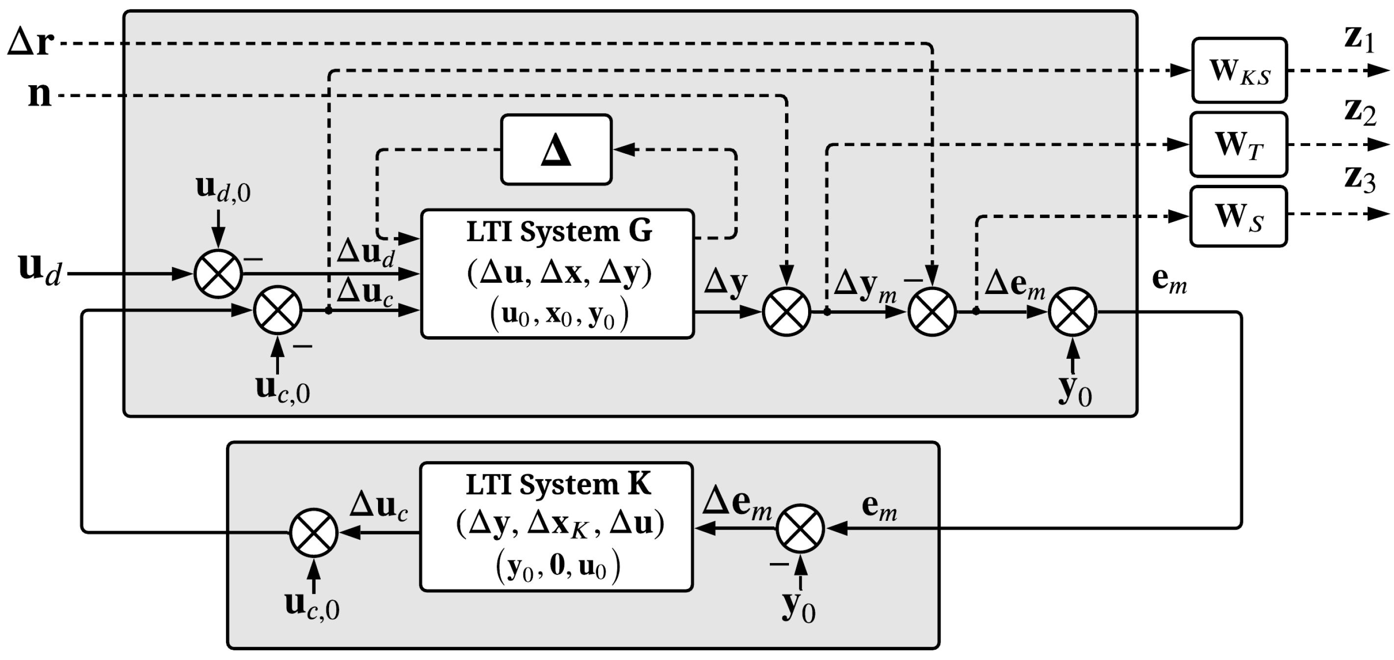
2.6. Robust Synthesis and Closed Loop Validation

Classical solutions to the H 2 / H problems are presented in [20,21,22,23,24] and others. The control problem is typically formulated for the nominal plant using the generalized framework depicted in Figure 5a.
This generalized plant is obtained by augmenting the physical process model with a set of mathematical signals which aid the optimization procedure and has the following structure:
z ( t ) y ( t ) = P 11 P 12 P 21 P 22 w ( t ) u ( t ) , with P 11 P 12 P 21 P 22 = A B 1 B 2 C 1 D 11 D 12 C 2 D 21 D 22 ,
where w R n w is the exogenous input vector, u R n u is the control input vector, z R n z is the error (output, performance) vector, and y R n y is the measurement vector. The closed loop system is given by the LLFT interconnection of P and K:
P z w = LLFT ( P , K ) = P 11 + P 12 K I P 22 K 1 P 21 .
For the nominal plant, the target of the robust control problem is to minimize the H norm using a stabilizing controller K, which can be written as
min K stab . P z w = min K stab . sup ω R + σ ¯ P z w ( j ω ) ,
obtaining a (sub)optimal value γ by iteration, which minimizes the effects of the input vector w ( t ) as seen through the performance output vector z ( t ) .
However, this problem ensures only nominal stability and nominal performance. However, the plant is a model of a physical process, having uncertainties. There are two types of uncertainties: unstructured, which illustrates neglected and unmodelled dynamics and which are represented by a full block Δ R m × m , and parametric, which are represented by δ I , where δ is the maximum bound of the variable parameter. In a mixed-scenario, the following set is considered:  
Δ = Δ = diag δ 1 I n 1 , , δ s I n s , Δ 1 , , Δ f | δ k R , Δ j R m j × m j , k = 1 , s ¯ , j = 1 , f ¯ .
In Figure 5b, the closed loop system containing a LLFT connection between plant P and controller K and an ULFT connection between plant P and uncertainty block Δ is presented. In this case, the generalized plant contains one extra input vector, i.e., disturbance inputs d R n d , and one extra output vector, i.e., disturbance outputs v R n v , giving the following structure:  
P Δ ( s ) = P v d ( s ) P v w ( s ) P v u ( s ) P z d ( s ) P z w ( s ) P z u ( s ) P y d ( s ) P y w ( s ) P y u ( s ) P Δ : x ˙ ( t ) v ( t ) z ( t ) y ( t ) = A B d B w B u C v D v d D v w D v u C z D z d D z w D z u C y D y d D y w D y u x ( t ) d ( t ) w ( t ) u ( t ) .
A mathematical tool used for studying the robustness is the structured singular value, defined for a square matrix M C N × N with respect to the set Δ as
μ Δ ( M ) = 1 min Δ Δ { σ ¯ ( Δ ) | det ( I M Δ ) = 0 } ,
if there exists Δ Δ such that the matrix I M Δ is rank deficient; otherwise, it is 0. For the system presented in Figure 5b, the structured singular value of LLFT ( P , K ) , according to Δ , can be defined as
μ Δ ( LLFT ( P , K ) ( s ) ) = sup ω R + μ Δ ( LLFT ( P , K ) ( j ω ) ) .
Besides the classical H 2 / H techniques, the μ synthesis framework manages to design a controller that meets the robust stability and robust performance specifications. The robust stability implies that a certain controller manages to stabilize all processes described by the upper linear fractional transformation between plant and uncertainty block, while the robust performance means that the controller is able to impose the desired closed loop performance in the worst-case scenario. Based on the main loop theorem, a controller K meets the robust stability and robust performance if and only if the structural singular value of the lower linear fractional transformation with respect to Δ is smaller than 1. Therefore, the minimization problem can be written as
inf K stab . sup ω R + μ Δ ( LLFT ( P , K ) ( j ω ) ) ,
which is not a convex problem. Additionally, the structural singular values are difficult to be explicitly computed. In order to solve this problem, the following upper bound is used [25]:
μ Δ ( LLFT ( P , K ) ( j ω ) ) inf D D σ ¯ ( D · LLFT ( P , K ) ( j ω ) · D 1 ) ,
where the set D is defined in relation to the uncertainty set Δ as  
D = diag D 1 , , D s , d 1 I m 1 , , d f I m f | D k = D k R n k × n k , d j > 0 , k = 1 , s ¯ , j = 1 , f ¯ .
Now, using this bound, the solution of the initial non-convex problem can be practically approximated by solving the following quasi-convex problem:
inf K stab . sup ω R + inf D D σ ¯ D ( j ω ) · LLFT ( P , K ) ( j ω ) · ( D ( j ω ) ) 1 .
Finally, if the system D is fixed, the problem (34) is nothing but a H control problem, in this case called the K step. Furthermore, for a fixed controller K, the D scale step can be obtained by solving a Parrot problem for a desired set of frequencies Ω = { ω 1 , , ω N } using a LMI and then obtain a minimum phase system after performing an identification step. Using these, an iterative algorithm, based on alternative D-K iterations, manages to solve the μ synthesis problem. This procedure starts with D = I and successively applies a K step and a D scaling step until a stopping criterion is reached.
Of great use in the controller design phase are the sensitivity, complementary sensitivity, and control effort functions, respectively, defined by
S : = I + G K 1 ;
T : = G K I + G K 1 ;
R : = K I + G K 1 = K S ,
where G is the open loop model. The great advantage of considering this approach is that it allows sculpting the relevant loop functions to impose steady-state and transitory regime performances, which are specified for different frequency ranges, using adequately selected weighting functions. Besides the minimization from Equation (34), different constraints can be added to the optimization problem to obtain a compromise between S, K S , and T at various frequencies:
inf K stab . sup ω R + inf D D σ ¯ D ( j ω ) · LLFT ( P , K ) ( j ω ) · ( D ( j ω ) ) 1 ,
such that W S S W T T W K S K S T < 1 ,
also known as the mixed-sensitivity closed loop shaping μ synthesis method. The approach considered in this first iteration of the toolbox uses closed loop shaping with μ synthesis for the controller. Using the work in [26] as a starting point, different frequency response specifications, directly correlated with desired time-response performances, can be imposed in the weighting functions. The sensitivity weighting function W S depends on four parameters as in
W S ( s ) = 1 M 1 / n s + ω B s + ω B A 1 / n n ,
where ω B represents the imposed bandwidth of the system; M imposes the H norm of the sensitivity function, in order to limit the overshoot of the system; n imposes the slope of the sensitivity function for low frequencies; and A imposes the maximum allowed steady-state error.
On the other hand, the complementary sensitivity weighting function W T can be generally defined by the following structure, in a symmetrical manner compared to W S :
W T ( s ) = s + ω B T A T 1 / n s + ω B T M T 1 / n n ,
with ω B T being the imposed bandwidth of the system; M T imposes the H norm of T ( s ) ; n imposes the roll-off slope of the closed loop system, which should be directly coupled with sensor noise characteristics; and A T imposes the least required attenuation for high frequencies. In practice, the complementary sensitivity bandwidth ω B T can be adapted to the characteristics of the sensor in order to account for high-frequency noise.
Finally, the control effort weighting function with desired specifications M 0 : = | W K S ( 0 ) | , M : = | W K S ( ) | and | W K S ( j · ω d ) | = M d , M 0 < M d < M can be synthesized by the following formula:
W K S ( s ) = M s + M 0 ω d M 2 M d 2 M d 2 M 0 2 s + ω d M 2 M d 2 M d 2 M 0 2 .
A higher-order counterpart can be generalized as for the previous cases, but was not found necessary for the proposed case studies and other tested benchmark plants.
Class RobustControlSynthesisProblem uses the nominal linearized plant around a required operating point using the system (14) and options (11)–(13), with a specified uncertainty type from Table 1, modeled through class UncertaintyBoundOptimization-Problem, allows imposing closed loop performance specifications with frequency weights (37)–(39), and synthesizes controller solutions for the problem (36) which cover the robust stability and robust performance problems. Additionally, the class also allows controller postprocessing, using order-reduction methods to compute easily implementable controllers. The aforementioned controller synthesis problem is illustrated in Figure 6, while the resulting LTI controller can be used in a MiL simulation context using the interface from class LTIEqSystem, encompassing system (3).
Class ClosedLoopControlProblem gathers all data, options, computations, and results from the previously presented individual blocks. It is used to define the end-to-end control problem by aggregating the uncertain plant family with its corresponding least conservative bound optimization; the robust control synthesis procedure and metadata; and allows Model-in-the-Loop simulations with the nonlinear, linearized, and hybrid system models, with automatic validation of imposed performances for the nonlinear plant in the frequency and time-domain alike.

3. Results

To showcase the ease of use and functionalities of the proposed toolbox, a set of case studies will be illustrated for DC-to-DC power converter circuits in a unified manner to encompass modeling, control synthesis and performance validation, considering the topologies buck, boost, and single-ended primary-inductor converter (SEPIC). DC-to-DC converters have been considered as a case study due to their ubiquity in various practical domains and applications, as presented in [27], ranging from renewable energy, hybrid and electric vehicles, controlled power sources, and many more. They can be seen as a good benchmark for control systems, due to their switching behavior, nonlinear dynamics, and different tried and tested control methods, such robust techniques in [28], Lyapunov methods in [29], passivity theory in [30], or sliding mode control as in [31].
This section will be split in a subsection which presents the converter mathematical models, a subsection with a suggested workflow for a general purpose control problem, followed by a subsection with numerical results and simulations for each of the studied converter topologies. For the SEPIC converter, having the most highly nonlinear behavior, thus being more difficult to control, we will illustrate and detail all plots generated by the toolbox, while for the buck and boost circuits, for brevity, we will show only the relevant figures and maintain the mathematical results and discussions.

3.1. Mathematical Modeling

The nonideal step-down (buck), step-up (boost), and single-ended primary-inductor converter (SEPIC) circuits are presented in Figure 7, where each component is described as follows.
  • S 1 : switching device, usually a transistor, and S 2 : switching device, usually a diode or transistor;
  • L, L 1 , L 2 : converter inductors;
  • C, C i n , C 1 , C 2 : converter capacitors;
  • R: (variable) output load resistance;
  • E: external source voltage;
  • r L , r L 1 , r L 2 : resistances associated with the inductors;
  • r C , r C i n , r C 1 , r C 2 : capacitors parasitic resistances;
  • r D S 1 , r D S 2 : resistances associated with the ON state of the switching devices (usually drain source);
  • V F 1 , V F 2 : constant voltage drops associated with the conducting phase of S 1 and S 2 ;
  • μ 0 , 1 : normalized duty cycle applied to S 1 ; complementary to the PWM signal applied to S 2 .
Each converter has one control switching device S 1 , while the other one, S 2 , will be complementary to the former. Although, typically S 2 is a diode, it is preferable to use two encapsulated transistors for S 1 and S 2 . When working in continuous conduction mode (CCM), all converters will have an ON state, corresponding to S 1 being on and S 2 off, along with an OFF state, for its complementary behavior. The corresponding LTI models, for a constant load resistance R, for the ON and OFF states will be presented using the following structure with the external voltage seen as disturbance input u ( t ) = E ( t ) , the voltage drops V F 1 and V F 2 as constant DC inputs, states from the inductor currents and capacitor voltages, and the load resistor voltage as measured output:
A B ¯ C D ¯ = A B B V C D D V ,
where:  
x ˙ = A O N x + B O N E + B V , O N V F 1 V F 2 ; y = C O N x + D O N E + D V , O N V F 1 V F 2 , x ˙ = A O F F x + B O F F E + B V , O F F V F 1 V F 2 ; y = C O F F x + D O F F E + D V , O F F V F 1 V F 2 .
The control variable is the duty cycle of the switching devices μ t     0 , 1 . Using a convex combination of the ON and OFF equation systems from Equation (41), an averaged state-space nonlinear model of the process is obtained close to the hybrid model’s behavior given a sufficiently high PWM frequency:
x ˙ ( t ) = μ ( t ) · x O N ( t ) + ( 1 μ ( t ) ) · x O F F ( t ) F x ( t ) , E ( t ) , R ( t ) , μ ( t ) T , t .
As such, an affine nonlinear system, with respect to μ , with the state function F as above can be implemented by inheriting the class System from the toolbox. The disturbances which affect the system are the voltage source E and variable output load R, which are stochastic in nature, along with uncertainties of its components due to manufacturing tolerances, relevant on inductors and capacitors. As the toolbox easily allows using the output capacitor voltage or output load voltage with minor modifications, we used the resistor voltage as measurement variable due to its corresponding practical control use cases. By inheriting the class UncertainPlantFactory, a set of tolerances can be imposed on all relevant circuit parameters and, also, an LTI uncertain set can be automatically computed with the provided mechanisms. The equilibrium point will have only the steady-state values of E ¯ , R ¯ , and u ¯ R imposed, with the following structure:
u ¯ , x ¯ , y ¯ = E ¯ , R ¯ , μ ¯ , i ¯ L 1 , u ¯ C 1 , , u ¯ R .
After synthesizing a robust controller, model-in-the-loop simulations would be desired for the averaged state-space models and, also, for a hybrid model description of the converters. For the hybrid approach, the class UncertainPlantFactory is inherited again, this time with individual plants of type HybridSystem. For the general approach for CCM, based on the structure from Equation (4), the input vector is comprised of u = E , R , μ T , the state vector is extended to x = z T , q , τ T , with z = i L 1 , u C 1 , T being the physical continuous states; q 0 , 1 the discrete state number, i.e., ON and OFF; and τ 0 , T P W M the time values for a single PWM period. After each PWM period completion, the auxiliary time state τ is reinitialized to 0. The model description becomes, for the state-space description
{ (44a) z ˙ ( t ) q ˙ ( t ) τ ˙ ( t ) = ( 1 q ) · A O N z ( t ) + B ¯ O N u ( t ) + q · A O F F z ( t ) + B ¯ O F F u ( t ) 0 1 , x , u , t C ; (44b) z + ( t ) q + ( t ) τ + ( t ) = z ( t ) 1 , if q = = 0 0 , if q = = 1 τ , if q = = 0 0 , if q = = 1 , x , u , t D ,
while the flow, jump, and output functions are
{ (45a) C x , u , t = q = = 0 τ μ ( t ) · T P W M q = = 1 τ > μ ( t ) · T P W M ; (45b) D x , u , t = q = = 0 τ > μ ( t ) · T P W M q = = 1 τ > T P W M ; (45c) y ( t ) = h x ( t ) , u ( t ) , t .
In order to encompass DCM regimes, the number of discrete states must be extended with new LTI blocks obtained by adding the mathematical constraint of canceling the diode S 2 voltage and, as such, the corresponding current signal for that branch, along with more sophisticated jump functions, flow and jump sets. For brevity, we will not insist on these extensions, although an example described for the boost converter can be found in [32].

3.2. Toolbox Workflow

A suggested end-to-end workflow for the toolbox can be summarized in the following steps, all of which should be run from intermediary methods of an instance of class ClosedLoopControlProblem:
  • inherit class System to define the nonlinear model of the process as in Equation (1) and Figure 1;
  • define equilibrium point specifications as in (11)–(13);
  • inherit class UncertainPlantFactory and overload method getRandomPlant;
  • using the desired operating point, linearize a set of systems using (16) and experimentally determine an uncertainty model W e x p based on Table 1;
  • define uncertainty options, including transfer function structure for all particles, and execute the methods from class UncertaintyBoundOptimizationProblem in order to minimize the functional J Ω , W e x p ( W x ) from Equation (21), obtaining W x , o p t ;
  • run optimization to compute the uncertainty weight W u n c ( s ) as in Table 1;
  • define robust control specifications W S , W T , and W K S as in Equations (37)–(39);
  • synthesize robust μ controller based on Figure 6;
  • apply order-reducing methods on the resulting controller;
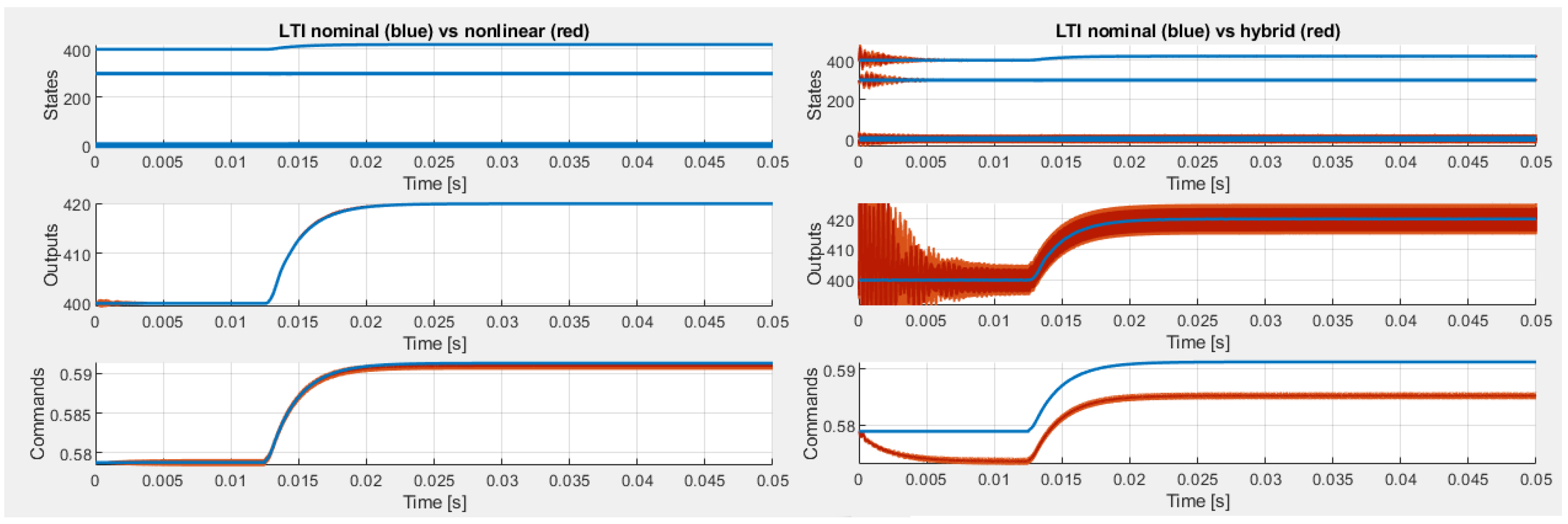
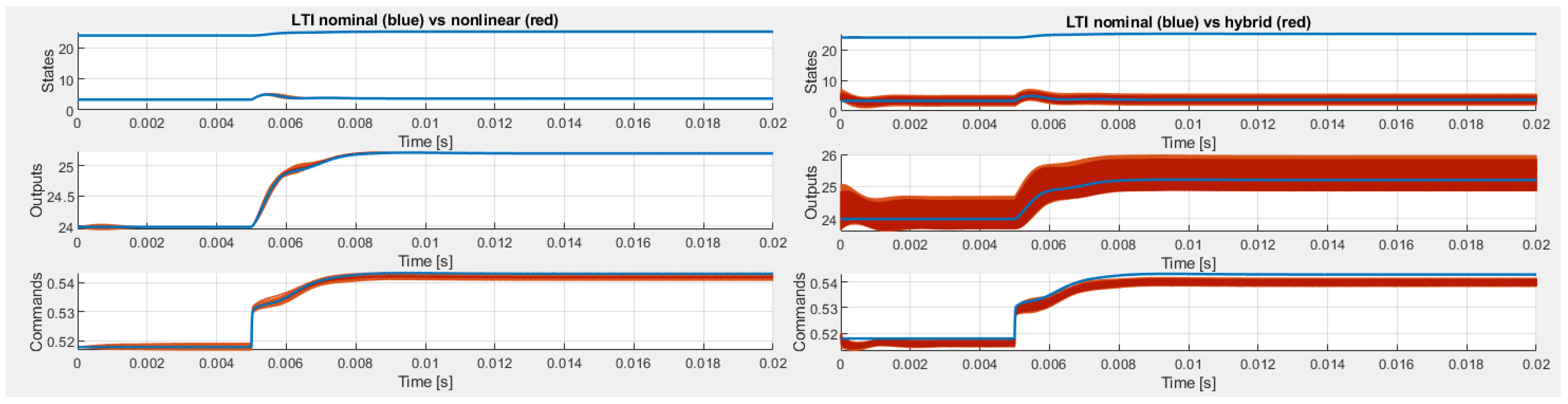
  • validate frequency and time-response performance specifications using the nonlinear system at operating point through Model-in-the-Loop simulations;
  • optionally, inherit the classes HybridSystem and UncertainPlantFactory, respectively, to validate time-response performance specifications using the corresponding hybrid plant model at operating point; for DC-to-DC converter control, the last step should be adapted for CCM or DCM operation.

3.3. Numerical Results

We will briefly present the obtained results for the three converters using the approaches established in Section 3.1 and Section 3.2.

3.3.1. SEPIC Converter

The SEPIC converter state-space model for the ON state of switch S 1 , as structured in Equation (41), is
1 r C i n C i n 0 0 0 0 1 r C i n C i n 0 0 1 L 1 r C i n + r L 1 + r D S 1 L 1 0 r D S 2 L 1 0 0 1 L 1 0 0 0 0 1 C 1 0 0 0 0 0 r D S 1 L 2 1 L 2 r D S 1 + r C 1 + r L 2 L 2 0 0 1 L 2 0 0 0 0 0 1 ( R + r C 2 ) C 2 0 0 0 0 0 0 0 R R + r C 2 0 0 0 ,
while for the OFF state of the switch S 1 is  
1 r C i n C i n 0 0 0 0 1 r C i n C i n 0 0 1 L 1 r a u x L 1 1 L 1 r D S 2 + r C 2 L 1 1 L 1 0 0 1 L 1 0 1 C 1 0 0 0 0 0 0 0 r D S 2 + r C 2 L 2 0 r D S 2 + r C 2 + r L 2 L 2 1 L 2 0 0 1 L 2 0 R ( R + r C 2 ) C 2 0 R ( R + r C 2 ) C 2 1 ( R + r C 2 ) C 2 0 0 0 0 r C R R + r C 0 r C R R + r C R R + r C 2 0 0 0 ,
with the auxiliary notation r a u x = r L 1 + r C 1 + r D S 1 + r C 2 + r C i n .
The nominal SEPIC converter parameters and their tolerances are presented in Table 2.
The desired operating point specifications are output signal y ( t ) u R ( t ) is at 400 [V], with nominal voltage source and load inputs u 1 ( t ) = E = 300 [V], u 2 ( t ) = R = 80 [ Ω ] . The initial guesses for the state equilibrium values where x ˜ = [ 30 , 0.5 , 30 , 0.5 , 30 ] and u 3 ( t ) = μ = 0.57 for the duty cycle control input. After computation, the actual equilibrium point is u , x , y   =   300 , 80 , 0.5788 , 300 , 6.8711 , 297.722 , 5 , 400 , 400 .
An input multiplicative uncertainty model, i.e., G ( s ) = G n ( s ) 1 + Δ ( s ) W u n c ( s ) , | | Δ | | 1 , as in Table 1 has been automatically computed from input u 3 ( t ) to output y 1 ( t ) , with tolerances ± 10 [V] and ± 5 [ Ω ] for inputs u 1 ( t ) = E and u 2 ( t ) = R , based on 1000 Monte Carlo simulations. The relevant frequencies vary in the interval ω ̲ = 10 2 , ω ¯ = 10 8 , with 300 equally distributed samples in log domain. A successful set of hyperparameters for the particle swarm optimization algorithm is comprised of a swarm size of 1000, initial swarm span of 10 4 , minimum neighbors fraction of 0.9 , and inertia range of 0.1 , 1.1 , for a transfer function structure as in Equation (19), with a complex pole pair and a complex zero pair, resulting in
W u n c ( s ) = 0.67275 s 2 + 941.1 s + 2.222 × 10 5 s 2 + 147.3 s + 5.422 × 10 7 .
The linearized SEPIC plant family is comprised of fourth-order stable systems, in minimal form, with four zeros, three of which are of nonminimum phase. The nominal model is
G n ( s ) = 4.1368 ( s + 8.003 e + 5 ) ( s + 2.304 e + 4 ) ( s 2 717.4 s + 5.145 e + 7 ) ( s 2 + 2673 s + 3.749 e + 7 ) ( s 2 + 1339 s + 6.493 e + 7 ) .
The entire uncertainty family has the same structure with poles, zeros, and equilibrium points in the vicinity of the nominal counterparts. The uncertain SEPIC plant family structure and behavior, along with the PSO conservative bound computation are illustrated in Figure 8. Figure 8-1 illustrates the pole-zero plot for the linearized uncertain SEPIC converter family, Figure 8-2 shows the best particle frequency-response fit W x ( s ) as in Equation (19) on the right y axis, and, also, the best functional fit on the left y axis, Figure 8-3 and Figure 8-4 show the frequency response of the plant G ( s ) family and uncertainty family Δ ( s ) W u n c ( s ) , respectively, while Figure 8-5 illustrates the system states and outputs for a 2 % step disturbance relative to the equilibrium input value μ 0 = 0.5788 .
For controller synthesis, the preferred loop shaping specifications were selected to highly penalize the control effort near the system resonance, as the obtained controllers would be difficult to implement in practice, needing high sampling frequencies, i.e., f e > 20 [kHz]. As such, for the sensitivity function: ω B = 200 [rad/s], A = 10 2 , M = 2 , n = 1 ; for the complementary sensitivity function: ω B T = 2000 [rad/s], A T = 10 4 , M T = 2 , n = 2 ; and for the control effort M 0 = 100 , M = 10 5 , | W K S ( j · 200 ) | = 250 , resulting in  
W S ( s ) = 0.5 s + 200 s + 2 , W T ( s ) = s 2 + 4000 s + 4 × 10 6 1 × 10 4 s 2 + 56.57 s + 8 × 10 6 , W K S ( s ) = 10 5 s + 8.729 × 10 6 s + 8.729 × 10 4 .
From the μ synthesis procedure, a controller of order 21 is obtained. After order reduction, the smallest controller which manages to assure all imposed specifications for the plant family, with a peak value μ Δ ( LLFT ( P , K ) ) 0.8361 < 1 , is given by the third-order system
K r e d S E P I C = 1.997 3.056 3.227 0.5018 3.057 2197 6118 0.3838 3.225 6118 1.016 × 10 4 0.4055 0.5018 0.3838 0.4055 0 .
The controller design phase, order reduction, and frequency response closed loop performance of the reduced-order one for the uncertain plant family are illustrated in Figure 9 and Figure 10. In this case, the control system has very large stability margins, with a phase margin of 82.1 [ ] and gain margin in the interval 19.4 , 20.3 [dB]. Additionally, as specified by the n = 2 and A T = 10 4 parameters of the complementary sensitivity weighting function, W T , the closed loop control system mitigates sensor noise signals with a considered spectrum starting from ω B T > 2000 [rad/s], using an initial roll-off of 40 [dB/dec], followed by an attenuation of at least four orders of magnitude. In the actual MiL simulations, the attenuation does not stop at the prescribed value, as the system manages to maintain at least a 20 [dB/dec] roll-off.
From Figure 11, the closed loop bandwidth can be observed as ω B > 200 [rad/s], equivalent to a rise time less than ≈5 [ms], a negligible steady-state error of ≈10 2 × ( y s s y 0 ) = 0.2 [V], where y s s represents the steady state value of the system, relative to the desired equilibrium value y 0 . Moreover, the system has no overshoot, and it behaves like a first-order low-pass filter by design. The nonlinear MiL simulation options are N = 50 random plants from the uncertainty set, solver is ode15i, due to the difficulty of simulating the closed loop plant otherwise (it is numerically unstable), with a step on the reference signal of 5 % from its initial equilibrium value of approximately 400 [V] and a simulation time of 0.05 [s]. Almost the same conditions apply to the hybrid MiL simulation, with the solver switched to ode113, as ode15i is not supported here, and a PWM period selected randomly for each experiment from a nominal value T P W M = 17.5 [s] with a ± 20 % fluctuation from one simulation to another. A comparison of the nonlinear and hybrid cases is presented also in Figure 11, where it can be seen that the transitory regime is practically identical, but for the hybrid case, a slightly lower command signal is necessary in steady state. Due to working with u R ( t ) instead of u C ( t ) only for the output signal, the current ripple is propagated into the measured voltage.

3.3.2. Buck Converter

The buck converter state-space models for the ON and OFF states of switch S 1 , respectively, as in Equation (41), are  
r p + r D S 1 L R ( R + r C ) L 1 L 1 L 0 R ( R + r C ) C 1 ( R + r C ) C 0 0 0 r C R R + r C R R + r C 0 0 0 ; r p r D S 2 L R ( R + r C ) L 0 0 1 L R ( R + r C ) C 1 ( R + r C ) C 0 0 0 r C R R + r C R R + r C 0 0 0 ,
with the auxiliary notation r p = r L + r C R R + r C = r L + r C | | R .
The nominal buck converter parameters and their tolerances are presented in Table 3.
The desired operating point specifications are as follows: the output signal y ( t ) u R ( t ) is at 5 [V], with nominal voltage source and load inputs u 1 ( t ) = E = 12 [V], u 2 ( t ) = R = 15 [ Ω ] . The initial guesses for the state equilibrium values where x ˜ = [ 1.25 , 5 ] and u 3 ( t ) = μ = 0.5 for the duty cycle control input. After computation, the actual equilibrium point is u , x , y = 12 , 15 , 0.4335 , 0.333 , 4.999 , 5 .
An input multiplicative uncertainty model, i.e., G ( s ) = G n ( s ) 1 + Δ ( s ) W u n c ( s ) , | | Δ | | 1 , as in Table 1, has been automatically computed from input u 3 ( t ) to output y 1 ( t ) , with tolerances ± 1 [V] and ± 1 [ Ω ] for inputs u 1 ( t ) = E and u 2 ( t ) = R , respectively, based on 1000 Monte Carlo simulations. The relevant frequencies vary in the interval ω ̲ = 10 1 , ω ¯ = 10 7 , with 200 equally distributed samples in log domain. A successful set of hyperparameters for the particle swarm optimization algorithm is comprised of a swarm size of 1000, initial swarm span of 10 4 , minimum neighbors fraction of 0.9 , and inertia range of 0.1 , 1.1 for a transfer function structure as in Equation (19), with a real pole and a real zero, resulting in
W u n c ( s ) = 0.51758 s + 510.5 s + 2906 .
The linearized buck plant family is comprised of second-order stable systems, in minimal form, with one zero. The nominal model is
G n ( s ) = 59178 ( s + 8333 ) s 2 + 5261 s + 4.114 × 10 7 .
The entire uncertainty family has the same structure with poles, zeros, and equilibrium points in the vicinity of the nominal counterparts. The uncertain buck plant family structure and behavior, along with the PSO conservative bound computation are illustrated in Figure 12.
For controller synthesis, the weighting function specifications were for the sensitivity function ω B = 1200 [rad/s], A = 10 4 , M = 2 , n = 1 ; for the complementary sensitivity function ω B T = 12 × 10 3 [rad/s], A T = 10 4 , M T = 2 , n = 2 ; and for the control effort M 0 = 0.1 , M = 100 , | W K S ( j · 1200 ) | = 2 , resulting in  
W S ( s ) = 0.5 s + 1200 s + 0.12 , W T ( s ) = s 2 + 24000 s + 1.44 × 10 8 1 × 10 4 s 2 + 339.4 s + 2.88 × 10 8 , W K S ( s ) = 100 s + 6006 s + 6.006 × 10 4 .
As specified by the n = 2 and A T = 10 4 parameters of the complementary sensitivity weighting function, W T , the closed loop control system mitigates sensor noise signals with a considered spectrum starting from ω B T > 12,000 [rad/s], using an initial roll-off of 40 [dB/dec], followed by an attenuation of at least four orders of magnitude. From the μ synthesis, a controller of order 17 is obtained. After order reduction, the smallest controller which manages to assure all imposed specifications for the plant family, with a peak μ Δ ( LLFT ( P , K ) ) 0.97 < 1 , is
K r e d B u c k = 0.12 0.003479 0.4751 12.68 0.0001768 2.304 1.241 × 10 4 0.1827 0.4611 1.241 × 10 4 4.522 × 10 4 25.09 12.68 0.1838 25.09 0 .
The nonlinear MiL simulation options are N = 50 random plants from the uncertainty set, with the ode23t solver, with a step on the reference signal of 5 % from its initial equilibrium value of approximately 5 [V] and a simulation time of 0.02 [s]. The simulation conditions for the hybrid MiL case are identical, with an additional PWM period selected randomly for each experiment from a nominal value T P W M = 17.5 [s] with a ± 20 % fluctuation from one simulation to another. A comparison of the nonlinear and hybrid cases is presented in Figure 13, where it can be seen that the transitory regime is practically identical. Due to working with u R ( t ) instead of u C ( t ) only for the output signal, the current ripple is propagated into the measured voltage.

3.3.3. Boost Converter

The boost converter state-space models for the ON and OFF states of switch S 1 , respectively, as in Equation (41), are  
r L + r D S 1 L 0 1 L 1 L 0 0 1 ( R + r C ) C 0 0 0 0 R R + r C 0 0 0 ; r a u x L R ( R + r C ) L 1 L 0 1 L R ( R + r C ) C 1 ( R + r C ) C 0 0 0 r C R R + r C R R + r C 0 0 0 ,
with the auxiliary notation r a u x = r L + r D S 2 + r C R R + r C = r L + r D S 2 + r C | | R . The nominal boost converter parameters and their tolerances are presented in Table 3, as they correspond with the buck converter parameters.
The desired operating point specifications are as follows: the output signal y ( t ) u R ( t ) is at 24 [V], with nominal voltage source and load inputs u 1 ( t ) = E = 12 [V], u 2 ( t ) = R = 15 [ Ω ] . The initial guesses for the state equilibrium values where x ˜ = [ 3 , 24 ] and u 3 ( t ) = μ = 0.5 for the duty cycle control input. After computation, the actual equilibrium point is u , x , y = 12 , 15 , 0.5179 , 0.3189 , 23.999 , 24 .
An input multiplicative uncertainty model, i.e., G ( s ) = G n ( s ) 1 + Δ ( s ) W u n c ( s ) , | | Δ | | 1 , as in Table 1, has been automatically computed from input u 3 ( t ) to output y 1 ( t ) , with tolerances ± 1 [V] and ± 1 [ Ω ] for inputs u 1 ( t ) = E and u 2 ( t ) = R , respectively, based on 1000 Monte Carlo simulations. The relevant frequencies vary in the interval ω ̲ = 10 1 , ω ¯ = 10 7 , with 200 equally distributed samples in log domain. A successful set of hyperparameters for the particle swarm optimization algorithm is comprised of a swarm size of 1500, initial swarm span of 10 4 , minimum neighbors fraction of 0.9 , and inertia range of 0.1 , 1.1 for a transfer function structure as in Equation (19), with two real poles and two real zeros, resulting in
W u n c ( s ) = 0.26592 s + 512.5 s + 3.535 × 10 4 s + 4016 s + 1.389 × 10 4 .
The linearized boost plant family is comprised of second-order stable systems, in minimal form, with two zeros, one being of nonminimum phase. The nominal model is
G n ( s ) = 0.65505 ( s + 8.551 × 10 4 ) ( s + 8333 ) s 2 + 2988 s + 9.746 × 10 6 .
The entire uncertainty family has the same structure with poles, zeros, and equilibrium points in the vicinity of the nominal counterparts. The uncertain boost plant family structure and behavior, along with the PSO least conservative second-order bound computation are illustrated in Figure 14.
For controller synthesis, the weighting function specifications were for the sensitivity function ω B = 650 [rad/s], A = 10 4 , M = 2 , n = 1 ; for the complementary sensitivity function ω B T = 3250 [rad/s], A T = 10 4 , M T = 2 , n = 1 ; and for the control effort M 0 = 0.1 , M = 100 , | W K S ( j · 650 ) | = 2 , resulting in
W S ( s ) = 0.5 s + 650 s + 0.065 , W T ( s ) = s + 3250 0.0001 s + 6500 , W K S ( s ) = 100 s + 3253 s + 3.252 × 10 4 .
An intrinsic limitation for the boost converter is that the bandwidth must not be imposed more than half of the value of the right-half plane non-minimum phase zero of the process, i.e., ω B z 2 43,000 [rad/s]. For this problem, this is a sufficiently high margin, as we also imposed a limitation for the command signal through W K S . As specified by the n = 2 and A T = 10 4 parameters of the complementary sensitivity weighting function, W T , the closed loop control system mitigates sensor noise signals with a considered spectrum starting from ω B T > 3250 [rad/s], using an initial roll-off of 40 [dB/dec], followed by an attenuation of at least four orders of magnitude. From the μ synthesis, a controller of order 17 is obtained. After order reduction, the smallest controller which retains all imposed specifications for the plant family, with a peak value μ Δ ( LLFT ( P , K ) ) 0.9547 < 1 , is
K r e d B o o s t = 0.065 0.8025 0.002966 5.007 0.7116 9.715 × 10 4 1.066 × 10 4 30.91 0.002575 1.065 × 10 4 1.422 0.113 5.007 30.91 0.1142 0 .
With this regulator, the boost converter control system with parameters from Table 3 has very large stability margins, with phase margins between 81 , 101 [ ] and gain margins in the interval 40 , 46 [dB]. The obtained sensitivity bandwidths vary between 828 , 2510 [rad/s], all of them better than the prespecified value of 800.
Nonlinear MiL simulation options are N = 50 random plants from the uncertainty set, with the ode15i solver, with a step on the reference signal of 5 % from its initial equilibrium value of approximately 5 [V] and a simulation time of 0.02 [s]. The simulation conditions for the hybrid MiL case are almost identical, with the use of the ode113 solver instead, set to a relative tolerance of 10 8 , and with an additional PWM period selected randomly for each experiment from a nominal value T P W M = 17.5 [s] with a ± 20 % fluctuation from one simulation to another. A comparison of the nonlinear and hybrid cases is presented in Figure 15, where it can be seen that the transitory regime is practically identical. Due to working with u R ( t ) instead of u C ( t ) only for the output signal, the current ripple is propagated into the measured voltage.

4. Conclusions and Future Work

There are several aspects to be discussed with regards to the presented toolbox and, additionally, including future work to be implemented in upcoming iterations.
The main reason for which the hybrid system framework is considered for the proposed toolbox is that the continuous-time plant needs to be regulated with a numerical controller. The hybrid system context may include LTI or nonlinear systems, switching systems (which are hybrid by nature), and singular systems, represented using differential-algebraic equations (DAEs). As such, for a continuous-time plant, a continuous-time controller is designed using the robust control framework. The controller is required to be numerically implementable, therefore two interfaces are necessary, which lead to a hybrid system. The numerical implementation must be easily obtained and automatically validated using rapid control prototyping (RCP) techniques. However, the properties of the closed loop system need to be reanalyzed after the discretization of the controller. Differential-algebraic equations represent a useful framework for modeling dynamical systems in engineering with a network-based structure of components. They are used in various industry fields such as mechanics (e.g., multiple-link mobile manipulator model), chemical engineering (modeling of chemical reactions), electrical engineering, cyber-physical systems, etc. All categories of processes taken into consideration in the hybrid framework are described using an approximate model that incorporates their relevant behavior. However, these types of systems have model and structure uncertainties. Moreover, the nonlinear systems that are linearized around an equilibrium point introduce such uncertainties as well. Therefore, to consider these uncertainties for the controller design, the robust control framework is mandatory. The first main applicability of RCP was to derive the necessary C/C++ source code with drivers for a given target microprocessor, and to simulate in reproducible conditions the behavior of a complex system. For the latter case, the most relevant simulation types, given in increasing order of complexity and closeness to reality, are Model-in-the-Loop (MiL), Software-in-the-Loop (SiL), and Hardware-in-the-Loop (HiL).
Many modeling software programs return circuits or mechanical systems already in DAE form, and it would be difficult, or sometimes impossible, to reformulate them in an ODE form without changing variables and losing their intended physical significance. In the context of the robust control framework used for DAEs, a significant work is the monograph in [33]. Although the robust control theory was well formulated in the previous years, this is still an open domain for research and publication, as surveyed and described in [34]. The difficulty of using methods which work correctly for multiple operating points is mitigated by using adaptive methods, such as gain scheduling for tracking problems. Furthermore, other relevant problems are automatic C/C++ code generation for controller implementation and the commutation between the prescribed operating points. Considering use cases for modeling, simulation, computer-aided design, and RCP, a relevant set of examples in the domain of power electronics, hybrid vehicles, and renewable energy systems is given in [35,36], where, although the main limitation is that analysis, control, and implementation aspects must be performed individually for the presented applications, they can be generally included under the same software framework, with the important exception of the robust control design and verification, along with the quantization sensitivity analysis in a unitary manner.
The main hindrance is that the majority of applications involve DAE systems of index greater than 1, meaning they necessitate more than one derivation step in order to formulate the problem, so there is a great need of tools that can also deal with high order DAEs, i.e., index 2 or 3 [37,38,39]. Another reason for the proposal of considering DAEs model is that they are also explicitly related to control issues, regarding both physical and operational constraints. Two illustrative examples are the case of improper systems, such as an ideal PID controller, and the elements that realize the decoupling in the MIMO systems case and when the plant has impulsive dynamics. The robust control techniques’ drawback is that the closed loop H 2 / H norm must be minimized using the prescribed weighting functions that penalize the exogenous outputs and these weighting functions need to be found ad hoc, which sometimes lead to some intermediary bad controllers and work overhead. Furthermore, after numerical implementation, the discrete controller loses a part of the imposed performances due to an inadequate sampling period or badly selected quantization levels. Although there are solutions in the literature, there is no unified approach to solve all these mentioned problems. As an extension to the framework and mindset given by the two previously mentioned RCP use cases, the current project proposed a highly automated toolbox for robust control design, which, in the current state-of-the-art is a highly iterative design process, when taking into consideration plant uncertainties, although the mathematical background for solving the optimization problems is well established. It proposes to eliminate design overhead when considering and modifying a specification set, manually redesigning the weighting functions, the optimization procedure, discretization of the regulators, quantization analysis, and closed loop analysis for the linearized and initial hybrid plant. Furthermore, in unison with high-performance numerical toolboxes, a justified report should automatically result after its use and explicitly state when unrealistic design specifications were considered.

Author Contributions

Conceptualization, M.Ş. and V.M.; methodology, M.Ş.; software, M.Ş.; validation, V.M. and P.D.; formal analysis, M.Ş. and P.D.; investigation, M.Ş. and M.S.; resources, M.Ş.; data curation, D.M.; writing—original draft preparation, M.Ş., M.S., and V.M.; writing—review and editing, V.M., D.M., and M.S.; visualization, M.Ş. and D.M.; supervision, P.D.; project administration, M.Ş.; funding acquisition, D.M. All authors have read and agreed to the published version of the manuscript.

Funding

This paper was supported by the Project “Entrepreneurial competences and excellence research in doctoral and postdoctoral programs—ANTREDOC”, project co-funded by the European Social Fund.

Conflicts of Interest

The authors declare no conflict of interest.

Sample Availability

Relevant source code implementation, including classes, objects, scripts, and data to reproduce the results presented in this paper are available from the GitHub repository: roconsys-toolbox-public.

Abbreviations

The following abbreviations are used in this manuscript:
CACSDComputer-Aided Control System Design
CCMContinuous Conduction Mode
DAEDifferential-Algebraic Equation
DCDirect Current
DCMDiscontinuous Conduction Mode
DOFDegree of Freedom
HyEQHybrid Equations Toolbox
LLFTLower Linear Fractional Transformation
LMILinear Matrix Inequality
LTILinear Time-Invariant
MiLModel-in-the-Loop
ODEOrdinary Differential Equation
PSOParticle Swarm Optimization
RCPRapid Control Prototyping
SEPICSingle-ended primary-inductor converter
ULFTUpper Linear Fractional Transformation

References

  1. Balas, G.; Chiang, R.; Packard, A.; Safonov, M. Robust Control Toolbox, Reference for MATLAB; The MathWorks, Inc.: Natick, MA, USA, 2020. [Google Scholar]
  2. Global Optimization Toolbox, User’s Guide for MATLAB; The MathWorks, Inc.: Natick, MA, USA, 2020.
  3. Feyel, P.; Duc, G.; Sandou, G. Optimal tuning of fixed-structure robust controller against multiple high-level requirements using evolutionary computation. Int. J. Robust Nonlinear Control 2019, 29, 949–972. [Google Scholar] [CrossRef]
  4. Blackwell, C.; Sastry, M.K.S. Multivar - A MATLAB based MIMO Control System Design Application. In Proceedings of the 8th International Conference on Computational Intelligence and Communication Networks, Tehri, India, 23–25 December 2016. [Google Scholar]
  5. Keller, P. Robust and optimal control in LabVIEW. IEEE Conf. Control. Technol. Appl. (CCTA) 2017. [Google Scholar] [CrossRef]
  6. Jacobs, L.; Verbandt, M.; De Preter, A.; Anthonis, J.; Swevers, J.; Pipeleers, G. A Toolbox for Robust Control Design: An Illustrative Case Study; IEEE: Tokyo, Japan, 2018. [Google Scholar]
  7. Sadeghpour, M.; de Oliveira, V.; Karimi, A. A Toolbox for Robust PID Controller Tuning Using Convex Optimization. IFAC Proc. Vol. 2012, 45, 158–163. [Google Scholar] [CrossRef] [Green Version]
  8. Ljung, L. System Identification Toolbox, Reference for MATLAB; The MathWorks, Inc.: Natick, MA, USA, 2020. [Google Scholar]
  9. Karimi, A.S. Frequency-Domain Robust Control Toolbox. In Proceedings of the 52nd IEEE Conference on Decision and Control, Firenze, Italy, 10–13 December 2013. [Google Scholar] [CrossRef] [Green Version]
  10. Sadeghzadeh, A.; Karimi, A.S. Fixed-structure 2 controller design for polytopic systems via LMIs. Optim. Control Appl. Meth. 2014. [Google Scholar] [CrossRef] [Green Version]
  11. Verbandt, M.; Swevers, J.; Pipeleers, G. An LTI control toolbox—Simplifying optimal feedback controller design. In Proceedings of the 2016 European Control Conference (ECC), Aalborg, Denmark, 29 June–1 July 2016. [Google Scholar] [CrossRef]
  12. Şuşcă, M. Solving Algebraic Riccati Equations Using Proper Deflating Subspaces for 2/ Synthesis. Master’s Thesis, Technical University of Cluj-Napoca, Cluj-Napoca, Romania, 2019. [Google Scholar] [CrossRef]
  13. Şuşcă, M.; Mihaly, V.; Stănese, M.; Dobra, P. Iterative Refinement Procedure for Solutions to Algebraic Riccati Equations. In Proceedings of the 2020 IEEE International Conference on Automation, Quality and Testing, Robotics (AQTR), Cluj-Napoca, Romania, 21–23 May 2020. [Google Scholar] [CrossRef]
  14. Mihaly, V. General Purpose Linear Matrix Inequality Solver With Applications in Robust and Nonlinear Control. Master’s Thesis, Technical University of Cluj-Napoca, Cluj-Napoca, Romania, 2020. [Google Scholar]
  15. Gumussoy, S.; Henrion, D.; Millstone, M.; Overton, M.L. Multiobjective Robust Control with HIFOO 2.0. In Proceedings of the 6th IFAC Symposium on Robust Control Design, Haifa, Israel, 16–18 June 2009. [Google Scholar]
  16. Sanfelice, R.G.; Copp, D.A.; Nanez, P. Hybrid Equations (HyEQ) Toolbox v2.04—A Toolbox for Simulating Hybrid Systems in MATLAB/Simulink®; MathWorks®: Natick, MA, USA, 2017. [Google Scholar]
  17. Goebel, R.; Sanfelice, R.G.; Teel, A.R. Hybrid Dynamical Systems: Modeling, Stability, and Robustness; Princeton University Press: Princeton, NJ, USA, 2012. [Google Scholar]
  18. Griewank, A.; Walther, A. Evaluating Derivatives: Principles and Techniques of Algorithmic Differentiation, 2nd ed.; SIAM: Philadelphia, PA, USA, 2008. [Google Scholar]
  19. Kennedy, J.; Eberhart, R. Particle swarm optimization. In Proceedings of the ICNN’95—International Conference on Neural Networks, Perth, WA, Australia, 27 November–1 December 1995; Volume 4, pp. 1942–1948. [Google Scholar] [CrossRef]
  20. Doyle, J.C.; Glover, K.; Khargonekar, P.P.; Francis, B.A. State-Space Solutions to Standard 2 and Control Problems. IEEE Trans. Autom. Control. 1989, 34, 831–847. [Google Scholar] [CrossRef]
  21. Fortuna, L.; Frasca, M. Optimal and Robust Control—Advanced Topics with MATLAB; CRC Press: Boca Raton, FL, USA, 2012. [Google Scholar]
  22. Gahinet, P.; Apkarian, P. A Linear Matrix Inequality Approach to Control. Int. J. Robust Nonlinear Control. 1994, 4, 421–448. [Google Scholar] [CrossRef]
  23. Ionescu, V.; Oară, C.; Weiss, M. Generalized Riccati Theory and Robust Control: A Popov Function Approach; John Wiley & Sons Ltd.: Chichester, UK, 1999. [Google Scholar]
  24. Zhou, K.; Doyle, J.C.; Glover, K. Robust and Optimal Control; Prentice Hall: Englewood Cliffs, NJ, USA, 1996. [Google Scholar]
  25. Packard, A.; Doyle, J.; Balas, G. Linear, Multivariable Robust Control With a μ Perspective. J. Dyn. Syst. Meas. Control. 1993, 115, 426–438. [Google Scholar] [CrossRef]
  26. Skogestad, S.; Postlethwaite, I. Multivariable Feedback Control: Analysis and Design, 2nd ed.; John Wiley & Sons Ltd.: Chichester, UK, 2005. [Google Scholar]
  27. Raghavendra, K.V.G.; Zeb, K.; Muthusamy, A.; Krishna, T.N.V.; Kumar, S.V.S.; Kim, D.-H.; Kim, M.-S.; Cho, H.-G.; Kim, H.-J. A Comprehensive Review of DC–DC Converter Topologies and Modulation Strategies with Recent Advances in Solar Photovoltaic Systems. Electronics 2020, 9, 31. [Google Scholar] [CrossRef] [Green Version]
  28. Chang, E.-C.; Cheng, C.-A.; Wu, R.-C. Robust Optimal Tracking Control of a Full-Bridge DC-AC. Converter. Appl. Sci. 2021, 11, 1211. [Google Scholar] [CrossRef]
  29. Garcia, G.; Lopez Santos, O. A Unified Approach for the Control of Power Electronics Converters. Part I—Stabilization and Regulation. Appl. Sci. 2021, 11, 631. [Google Scholar] [CrossRef]
  30. Mihaly, V.; Şuşcă, M.; Dobra, P. Passivity-Based Controller for Nonideal DC-to-DC Boost Converter. In Proceedings of the 2019 22nd International Conference on Control Systems and Computer Science (CSCS), Bucharest, Romania, 28–30 May 2019; pp. 30–35. [Google Scholar] [CrossRef]
  31. Repecho, V.; Biel, D.; Olm, J.M.; Fossas, E. Robust sliding mode control of a DC/DC Boost converter with switching frequency regulation. J. Frankl. Inst. 2018, 355, 5367–5383. [Google Scholar] [CrossRef]
  32. Lunze, I.; Lagarrigue, F.L. Handbook of Hybrid Systems Control: Theory, Tools, Applications; Cambridge University Press: Cambridge, UK, 2009. [Google Scholar]
  33. Feng, Y.; Yagoubi, M. Robust Control of Linear Descriptor Systems; Studies in Systems, Decision and Control 102; Springer: Singapore, 2017. [Google Scholar]
  34. Liu, K.-Z.; Yao, Y. ROBUST CONTROL—Theory and Applications; John Wiley & Sons (Asia) Pte Ltd.: Singapore, 2016. [Google Scholar]
  35. Zamboni, W.; Petrone, G. (Eds.) ELECTRIMACS 2019, Selected Papers—Volume 1; Springer International Publishing: Cham, Switzerland, 2020. [Google Scholar]
  36. Zamboni, W.; Petrone, G. (Eds.) ELECTRIMACS 2019, Selected Papers–Volume 2; Springer International Publishing: Cham, Switzerland, 2020. [Google Scholar]
  37. Ascher, U.M.; Petzold, L.R. Computer Methods for Ordinary Differential Equations and Differential-Algebraic Equations; SIAM: Philadelphia, PA, USA, 1998. [Google Scholar]
  38. Brenan, K.E.; Campbell, S.L.; Petzold, L.R. Numerical Solution of Initial-Value Problems in Differential-Algebraic Equations; SIAM Classics in Applied Mathematics: Philadelphia, PA, USA, 1996. [Google Scholar]
  39. Milano, F.; Dassios, I.; Liu, M.; Tzounas, G. Eigenvalue Problems in Power Systems; CRC Press: Boca Raton, FL, USA, 2021. [Google Scholar]
Figure 1. Class diagram for general-purpose nonlinear, LTI, linearized, and hybrid system implementations, along with the uncertain plant factory class, interconnections, and main functionalities.
Mathematics 09 00731 g001
Figure 2. Series and parallel interconnections for general-purpose and hybrid systems.
Mathematics 09 00731 g002
Figure 3. Upper (ULFT) and lower (LLFT) linear fractional transformation interconnections for general-purpose nonlinear and hybrid systems, with the ability to impose external reference signals.
Mathematics 09 00731 g003
Figure 4. Closed loop control problem class which encompasses an uncertain plant set with operating point specification, options for automatically modeling the plant uncertainty, specifying robust control performances, synthesizing controller, and validating obtained results.
Mathematics 09 00731 g004
Figure 5. (a) Generalized plant framework; (b) generalized plant framework with uncertainties.
Mathematics 09 00731 g005
Figure 6. Robust controller synthesis diagram for the plant G, with the uncertainty set Δ determined a priori using the functionality from Section 2.5, linearized at the operating point u 0 , x 0 , y 0 ; by convention, control inputs Δ u c of the linearized plant G are indexed after disturbance inputs Δ u d .
Mathematics 09 00731 g006
Figure 7. DC-to-DC power converter circuit topologies considered in the case studies: step-down (buck), step-up (boost), and single-ended primary-inductor (SEPIC).
Mathematics 09 00731 g007
Figure 8. SEPIC multiplicative uncertainty set computation and open loop responses for the operating point with E = 300 [ V ] , R = 80 [ Ω ] , U R = 400 [ V ] : step and frequency response, pole-zero placement; the step response is simulated for nonlinear plants sampled using UncertainPlantFactory.
Mathematics 09 00731 g008
Figure 9. SEPIC-synthesized (order 21) vs. reduced (order 3) controllers; the peak μ value does not monotonically decrease with respect to controller order due to the influence of the ≈3750 [rad/s] notch over the converter resonance, which was not taken into account by the order reduction mechanism.
Mathematics 09 00731 g009
Figure 10. SEPIC open loop plant family with S, T, and K S functions using the reduced-order controller, which retains all imposed performance specifications for all test cases, provides high phase and gain margins, and guarantees closed loop response practically similar to that of a first-order low-pass filter; a relatively low bandwidth was imposed to compensate the SEPIC converter resonance and presence of multiple nonminimum phase zeros.
Mathematics 09 00731 g010
Figure 11. SEPIC-averaged state-space and hybrid model Monte Carlo closed loop simulations; due to a relatively low bandwidth imposed in order to obtain good stability margins and easily implementable controllers, all plants respond almost identically, although component tolerances reach values of ± 20 % ; the initial transients exist due to starting the simulations from the nominal equilibrium point only.
Mathematics 09 00731 g011
Figure 12. Buck multiplicative uncertainty set computation and open loop responses for the operating point with E = 12 [ V ] , R = 15 [ Ω ] , U R = 5 [ V ] : step and frequency response, pole-zero placement; the step response is simulated for nonlinear plants sampled using UncertainPlantFactory.
Mathematics 09 00731 g012
Figure 13. Buck averaged state-space and hybrid model Monte Carlo closed loop simulations with a closed loop bandwidth ω B > 1200 [rad/s], equivalent to a rise time of ≈0.83 [ms], negligible steady-state error, and no overshoot.
Mathematics 09 00731 g013
Figure 14. Boost multiplicative uncertainty set computation and open loop responses for the operating point with E = 12 [ V ] , R = 15 [ Ω ] , U R = 24 [ V ] : step and frequency response, pole-zero placement; the step response is simulated for nonlinear plants sampled using UncertainPlantFactory.
Mathematics 09 00731 g014
Figure 15. Boost averaged state-space and hybrid model Monte Carlo closed loop simulations with a closed loop bandwidth ω B > 650 [rad/s], equivalent to a rise time less than ≈1.53 [ms], negligible steady-state error and no overshoot.
Mathematics 09 00731 g015
Table 1. Commonly used classes of perturbation and uncertainty models for multiple-input and multiple-output (MIMO) systems, implemented in class UncertainPlantFactory.
Uncertainty TypeDefinitionImplementation
Additive G ( s ) = G n ( s ) + Δ ( s ) Δ ( s ) = G ( s ) G n ( s )
Inverse additive ( G ( s ) ) 1 = ( G n ( s ) ) 1 + Δ ( s ) Δ ( s ) = ( G ( s ) ) 1 ( G n ( s ) ) 1
Input multiplicative G ( s ) = G n ( s ) I + Δ ( s ) Δ ( s ) = ( G n ( s ) ) 1 G ( s ) G n ( s )
Output multiplicative G ( s ) =   I + Δ ( s ) G n ( s ) Δ ( s ) =   G ( s ) G n ( s ) ( G n ( s ) ) 1
Inverse input multiplicative ( G ( s ) ) 1 =   I + Δ ( s ) ( G n ( s ) ) 1 Δ ( s ) = ( G ( s ) ) 1 ( G n ( s ) ) I
Inverse output multiplicative ( G ( s ) ) 1 =   G n ( s ) 1 I + Δ ( s ) Δ ( s ) =   G n ( s ) G ( s ) 1 I
Left coprime factor G ( s ) =   M ˜ + Δ M ˜ 1 N ˜ + Δ N ˜ Δ M ˜ =   N ˜ + Δ N ˜ ( G ( s ) ) 1 M ˜ , 1 - DOF
Right coprime factor G ( s ) =   N + Δ N M + Δ M 1 Δ M =   G ( s ) 1 N + Δ N M , 1 - DOF
Table 2. Single-ended primary-inductor converter (SEPIC) converter parameters, values, and corresponding tolerances.
Param.Val.Tol.Param.Val.Tol.
L 1 2.57 [mH] ± 20 % L 2 1.71[mH] ± 20 %
r L 1 130 [m Ω ] ± 10 % r L 2 110 [m Ω ] ± 10 %
r D S 1 0.01 [ Ω ] ± 10 % r D S 2 80 [m Ω ] ± 10 %
C 1 4.7 [μF] ± 20 % C 2 3.57 [μF] ± 20 %
r C 1 270 [m Ω ] ± 10 % r C 2 350 [m Ω ] ± 10 %
C i n 3.57 [μF] ± 20 % r C i n 270 [m Ω ] ± 10 %
V F 1 0.2 [V] ± 10 % V F 2 0.62 [V] ± 10 %
Table 3. Buck and boost converter parameters, values, and corresponding tolerances.
Param.Val.Tol.Param.Val.Tol.
L40 [μH] ± 20 % r L 10 [m Ω ] ± 10 %
C600 [μF] ± 20 % r C 0.2 [ Ω ] ± 10 %
r D S 1 0.01 [ Ω ] ± 10 % r D S 2 0.01 [ Ω ] ± 10 %
V F 1 0.2 [V] ± 10 % V F 2 0.2 [V] ± 10 %
Publisher’s Note: MDPI stays neutral with regard to jurisdictional claims in published maps and institutional affiliations.

