Article

A Family of Functionally-Fitted Third Derivative Block Falkner Methods for Solving Second-Order Initial-Value Problems with Oscillating Solutions

1
Department of Applied Mathematics, Universidad de Salamanca, 37008 Salamanca, Spain
2
Distance Learning Institute, University of Lagos, Lagos Mainland 101017, Nigeria
3
Department of Mathematics, University of Lagos, Lagos Mainland 101017, Nigeria
4
Department of Mathematics and Statistics, Austin Peay State University, Clarksville, TN 37044, USA
*
Author to whom correspondence should be addressed.
These authors contributed equally to this work.
Mathematics 2021, 9(7), 713; https://doi.org/10.3390/math9070713
Submission received: 25 February 2021 / Revised: 22 March 2021 / Accepted: 23 March 2021 / Published: 25 March 2021
(This article belongs to the Special Issue Numerical Methods for Solving Differential Problems)

Abstract

:
One of the well-known schemes for the direct numerical integration of second-order initial-value problems is due to Falkner. This paper focuses on the construction of a family of adapted block Falkner methods which are frequency dependent for the direct numerical solution of second-order initial value problems with oscillatory solutions. The techniques of collocation and interpolation are adopted here to derive the new methods. The study of the properties of the proposed adapted block Falkner methods reveals that they are consistent and zero-stable, and thus, convergent. Furthermore, the stability analysis and the algebraic order conditions of the proposed methods are established. As may be seen from the numerical results, the resulting family is efficient and competitive compared to some recent methods in the literature.

1. Introduction

The numerical integration of initial value problems (IVPs) of second order ordinary differential equations (ODEs) has attracted the attention of researchers in the field for decades. The importance of such problems is their use in the applied sciences to model different phenomena such as the mass movement under the action of a force, problems of orbital dynamics, molecular dynamics, circuit theory, control theory, or quantum mechanics among others. It turns out that most of these problems do not have closed-form solutions, and consequently it is important to develop numerical methods that can solve them directly. Accordingly, several numerical methods for solving second-order IVPs that do not contain the first derivative have been investigated by Lambert and Watson [1], Ananthakrishnaiah [2], Simos [3], Hairer et al. [4], Tsitouras et al. ([5,6]), Wang et al. ([7,8]), Franco ([9,10]), Ramos and Patricio [11], Chen et al. [12], Shi and Wu [13], Fang et al. [14], Senu et al. [15] among others.
Recently, some researchers have considered the direct integration of the general second order IVPs containing the first derivative. This can be found in the works by Guo and Yan [16], Vigo-Aguiar and Ramos [17], Jator et al. ([18,19]), Mahmoud and Osman [20], Awoyemi [21], Liu and Wu [22], You et al. [23], Li et al. [24], Chen et al. [25], Li et al. [26], and You et al. [27]. The implementation of some of these methods is based on a step-by-step fashion, while others are implemented in predictor-corrector modes. In either case, the cost of execution increases, especially, for higher-order methods. It turns out that some of these methods do not take advantage of the oscillatory or even periodic behavior of the solutions. If the period is known or can be estimated in advance this could be considered in the development of the method in order to improve its performance.
One of the numerical integrators for the general second order IVP in which the first derivative appears explicitly is an explicit method due to Falkner [28], while the implicit form is due to Collatz [29]. Some modifications of the Falkner methods have appeared in the literature (see [30,31,32,33]). The adapted Falkner methods take advantage of the special periodic feature of the solution of the IVP, and can be found in the works by Li and Wu [34], Li [35], and Ehigie and Okunuga [36]. The use of adapted methods started with the elegant work by Gautchi [37] and later by Lyche [38]. Many extensions of these have been investigated by Franco ([39,40]), Ixaru et al. [41], Vanden Berghe and Van Daele [42], Jator et al. [43], Jator ([18,44]), Ramos and Vigo-Aguiar [45], Vigo-Aguiar and Ramos ([46,47]), Coleman and Duxbury [48], Coleman and Ixaru [49], Nguyen et al. [50], Ozawa [51], Fang et al. [14], Franco and Gomez [52], Wua and Tian [53]. Nonetheless, most of these methods have been implemented in a step-by-step procedure. Also, in all these extensions, the basis function considered is either the set { 1 , x , x 2 , , x n , exp ( ω x ) , exp ( ω x ) } or { 1 , x , x 2 , , x n , sin ( ω x ) , cos ( ω x ) } .
In the current article, we propose a class of Functionally-Fitted third derivative Block Falkner Methods (BFFM) for the direct integration of the general second order initial value problem whose solution is oscillatory or periodic, in the latter case with the frequency known, or that can be estimated in advance. This class, which is an adapted formulation of the methods in Ramos and Rufai [33], uses a basis function different from what can be seen in the reviewed literature. We emphasize that this method is different from the methods by Jator ([18,44]); whereas our methods are implicit Falkner methods whose coefficients are trigonometric and hyperbolic functions depending on the fitting frequency, ω , and the step size, h, the methods by Jator ([18,44]) present trigonometric coefficients. It is important to note here that the accuracy in estimating this frequency is crucial in adapted numerical methods, as shown in [45].
The rest of this paper is organized as follows: the derivation of BFFM is presented in Section 2. The analysis of the characteristics of the BFFM is discussed in Section 3 while some numerical experiments are presented in Section 4. Finally, we give some concluding remarks in Section 5.

2. Development of the BFFM

Consider the general second order IVP of the form
y = f ( x , y , y ) , y ( x 0 ) = y 0 , y ( x 0 ) = y 0 , x [ x 0 , x N ] R ,
whose solution is oscillatory or periodic with the frequency approximately known in advance and f : [ x 0 , x N ] × R 2 s R s is a smooth function that satisfies a Lipschitz condition and s is the dimension of the system. For the development of the method, y ( x ) is taken as a scalar function although as we will see in the numerical experiments, the method may be applied in a component wise mode to solve differential systems. We now set-out some useful definitions related with the methods in Ramos and Rufai [33], that will aid the derivation of the BFFM.
Definition 1.
The continuous formulation of the adapted k—step third derivative Falkner method for approximating the solution of Equation (1) is defined by
y ¯ ( x ) = α k 0 ( x , u ) y n + 1 + h α k 1 ( x , u ) y n + 1 + h 2 j = 0 k β k j ( x , u ) f n + j + h 3 γ k ( x , u ) g n + k ,
where the coefficients α k 0 ( x , u ) , α k 1 ( x , u ) , β k j ( x , u ) and γ k ( x , u ) are functions of x and u = ω h , being ω the frequency of the method (see [45]), and g ( x , y , y ) = y ( x ) = f x ( x , y , y ) + f y ( x , y , y ) y ( x ) + f y ( x , y , y ) f ( x , y , y ) .
Definition 2.
The primary formulas of the adapted k—step third derivative block Falkner method for the numerical solution of Equation (1) are given by
{ y n + k = y n + 1 + ( k 1 ) h y n + 1 + h 2 j = 0 k β k j ( u ) f n + j + h 3 γ k ( u ) g n + k h y n + k = h y n + 1 + h 2 j = 0 k β ¯ k j ( u ) f n + j + h 3 γ ¯ k i ( u ) g n + k .
In these formulas, y n + j , y n + j , f n + j and g n + k are numerical approximations to the exact values y ( x n + j ) , y ( x n + j ) , f ( x n + j , y ( x n + j ) , y ( x n + j ) ) and g ( x n + j , y ( x n + j ) , y ( x n + j ) ) , respectively, with x n + j = x n + j h discrete points on [ x 0 , x N ] being h a fixed stepsize. The coefficients β k j , γ k and β ¯ k j , γ ¯ k depend on the parameter u and are obtained after evaluating the fitting function I ( x ) in Theorem 1 and its derivative, respectively, at x n + k .
Definition 3.
The ( 2 k 2 ) secondary formulas of the adapted k—step third derivative block Falkner method for the numerical solution of Equation (1) are given by
{ y n + μ = y n + 1 + ( μ 1 ) h y n + 1 + h 2 j = 0 k β k j μ ( u ) f n + j + h 3 γ k μ ( u ) g n + k h y n + μ = h y n + 1 + h 2 j = 0 k β ¯ k j μ ( u ) f n + j + h 3 γ ¯ k μ ( u ) g n + k ,
where μ = 0 , 2 , 3 , , ( k 1 ) .
Again, the coefficients β k j μ , γ k μ and β ¯ k j μ , γ ¯ k μ depend on u, and are obtained after evaluating the fitting function I ( x ) and its derivative at x n + μ , μ = 0 , 2 , 3 , , ( k 1 ) .
Definition 4.
The adapted k—step third derivative block Falkner method consists of the primary formulas in (3) and the secondary formulas in (4), which form the BFFM.

2.1. Derivation of the BFFM

Let Ω = { π 0 ( x ) , π 1 ( x ) , π 2 ( x ) , , π k + 3 ( x ) } be a set of k + 4 linearly independent functions. We seek an approximate solution I ( x ) s p a n ( Ω ) , called a fitted function associated to the adapted Falkner method, which satisfies the IVP in Equation (1) at some specified points.
The coefficients of the adapted Falkner method depend on the nature of the fitting function I ( x ) accordingly on how the set Ω is chosen, which can be any of the types listed in Nguyen et al. [50], where for any of the choices we have to take a total of k + 4 elements to determine the adapted block Falkner method on the basis that the approximations are of the form in (2). In order to develop the adapted Falkner methods in this paper we choose Ω as
Ω = { 1 , x , , x k 1 } { sin ( ω x ) , cos ( ω x ) } { sinh ( ω x ) , cosh ( ω x ) } .
To get the coefficients of the fitting function associated to the set Ω in (5), I ( x ) is interpolated at the point x = x n + 1 , and the following collocating conditions are considered: I ( x ) at x = x n + 1 , I ( x ) at the points x = x n + j , j = 0 , 1 , , k , and I ( x ) at x = x n + k . This leads to the following system of k + 4 equations
{ I ( x n + 1 ) = y n + 1 , I ( x n + 1 ) = y n + 1 , I ( x n + j ) = f n + j , j = 0 , 1 , , k , I ( x n + k ) = g n + k .
Theorem 1.
Let I ( x ) be the fitting function associated to the set Ω in (5),
{ P i ( x ) } i = 0 k + 3 = { 1 , x , , x k 1 , sin ( ω x ) , cos ( ω x ) , sinh ( ω x ) , cosh ( ω x ) } ,
and the vector Λ = ( y n + 1 , y n + 1 , f n , f n + 1 , , f n + k , g n + k ) T , where T denotes the transpose. Consider the following square matrix of dimension k + 4 which is the matrix of coefficients of the system in (6),
Π = [ P 0 ( x n + 1 ) P 1 ( x n + 1 ) P k + 3 ( x n + 1 ) P 0 ( x n + 1 ) P 1 ( x n + 1 ) P k + 3 ( x n + 1 ) P 0 ( x n ) P 1 ( x n ) P k + 3 ( x n ) P 0 ( x n + k ) P 1 ( x n + k ) P k + 3 ( x n + k ) P 0 ( x n + k ) P 1 ( x n + k ) P k + 3 ( x n + k ) ] ,
and Π i obtained by replacing the i-th column of Π by the vector Λ. If we impose that I ( x ) satisfies the system of k + 4 equations in (6), then it can be written as
I ( x ) = i = 0 k + 3 d e t ( Π i ) d e t ( Π ) P i ( x ) .
Proof. 
The proof can be readily obtained, similarly to the one given in Jator [18] with slight modifications in notations. □
Remark 1.
As an illustration of the theoretical result in the above theorem, the explicit form of the matrix Π and d e t ( Π i ) are provided in the Appendix A for k = 2 .

2.2. Specification of the BFFM

We emphasize that for each k, there are two primary formulas of the form in Equation (3) and 2 k 2 secondary formulas as those in Equation (4) (which are obtained by evaluating the fitting function in (7) at the corresponding points) that combined together form the proposed BFFM. Hence the BFFM has 2 k formulas.
As an illustration, we specified how to obtain the BFFM for k = 2 and k = 3 , repectively.
For k = 2 , we evaluate the fitting function in (7) and its first derivative at x = { x n + 2 , x n } to obtain the two primary formulas and the two secondary formulas as
{ y n + 2 = y n + 1 + h y n + 1 + h 2 j = 0 2 β 2 j ( u ) f n + j + h 3 γ 2 ( u ) g n + 2 h y n + 2 = h y n + 1 + h 2 j = 0 2 β ¯ 2 j f n + j ( u ) + h 3 γ ¯ 2 ( u ) g n + 2 y n = y n + 1 h y n + 1 + h 2 j = 0 2 β 2 j 0 ( u ) f n + j + h 3 γ 2 0 ( u ) g n + 2 h y n = h y n + 1 + h 2 j = 0 2 β ¯ 2 j 0 ( u ) f n + j + h 3 γ ¯ 2 0 ( u ) g n + 2 .
Whereas for k = 3 , we evaluate the fitting function in (7) and its first derivative at x = x n + 3 and then at x = { x n + 2 , x n } to obtain the two primary formulas and the four secondary formulas, which result in the following
{ y n + 3 = y n + 1 + 2 h y n + 1 + h 2 j = 0 3 β 3 j ( u ) f n + j + h 3 γ 3 ( u ) g n + 3 h y n + 3 = h y n + 1 + h 2 j = 0 3 β ¯ 3 j f n + j ( u ) + h 3 γ ¯ 3 ( u ) g n + 3 y n + 2 = y n + 1 + h y n + 1 + h 2 j = 0 3 β 3 j 2 ( u ) f n + j + h 3 γ 3 2 ( u ) g n + 3 h y n + 2 = h y n + 1 + h 2 j = 0 3 β ¯ 3 j 2 ( u ) f n + j + h 3 γ ¯ 3 2 ( u ) g n + 3 y n = y n + 1 h y n + 1 + h 2 j = 0 3 β 3 j 0 ( u ) f n + j + h 3 γ 3 0 ( u ) g n + 3 h y n = h y n + 1 + h 2 j = 0 3 β ¯ 3 j 0 ( u ) f n + j + h 3 γ ¯ 3 0 ( u ) g n + 3 .
Remark 2.
For small values of u, the coefficients of the BFFM may be subject to heavy cancellations. In that case the Taylor series expansion of the coefficients is preferable (see Lambert, [54]). Specific coefficients of the two primary formulas and their corresponding series expansion up to O ( u 16 ) for k = 2 are provided in Appendix B.
Remark 3.
When u 0 , the formulas in Equations (8) and (9) reduce to the conventional third derivative Falkner formulas for k = 2 and k = 3 , respectively, in Ramos and Rufai [33].

3. Analysis of the BFFM

We discuss the basic analysis of the proposed BFFM in this section. The analysis includes the Algebraic Order, Local Truncation Error, Consistency, Zero-Stability, Convergence and Linear Stability of the BFFM.

3.1. Algebraic Order, Local Truncation Errors and Consistency of the BFFM

The purpose of this subsection is to establish the uniform algebraic order for each of the formulas that form the BFFM and their corresponding local truncation errors with the aid of the theory of linear operators (Lambert [54]).

3.1.1. Local Truncation Error of BFFM

Proposition 1.
The local truncation error of each formula of the k—step BFFM is of the form C k + 4 h k + 4 ( ω 4 y k ( x n ) y ( k + 4 ) ( x n ) ) + O ( h k + 5 ) , where C k + 4 is the error constant.
Proof. 
Since the block Falkner formulas in Equations (3) and (4) are made up of generalized linear multistep formulas, we associate the Falkner formulas with linear difference operators L [ y ( x n ) ; h ] , L [ y ( x n ) ; h ] for the primary formulas and L μ [ y ( x n ) ; h ] , L μ [ y ( x n ) ; h ] , μ = { 0 , 2 , 3 , , k 1 } , for the secondary formulas, defined respectively by
L [ y ( x n ) ; h ] = y ( x n + k h ) y ( x n + h ) ( k 1 ) h y ( x n + h ) h 2 j = 0 k β k j ( u ) y ( x n + j h ) h 3 γ k ( u ) y ( x n + k h ) , L [ y ( x n ) ; h ] = h y ( x n + k h ) h y ( x n + h ) h 2 j = 0 k β ¯ k j ( u ) y ( x n + j h ) h 3 γ ¯ k ( u ) y ( x n + k h ) , L μ [ y ( x n ) ; h ] = y ( x n + μ h ) y ( x n + h ) ( μ 1 ) h y ( x n + h ) h 2 j = 0 k β k j μ ( u ) y ( x n + j h ) h 3 γ k μ ( u ) y ( x n + k h ) , L μ [ y ( x n ) ; h ] = h y ( x n + μ h ) h y ( x n + h ) h 2 j = 0 k β ¯ k j μ ( u ) y ( x n + j h ) h 3 γ ¯ k μ ( u ) y ( x n + k h ) .
Consider the Taylor series expansions of the right hand sides of the above formulas in powers of h. It can be shown that the first non zero term is of the form C k + 4 h k + 4 ( y ( k + 4 ) ( x n ) ω 4 y ( k ) ( x n ) ) + O ( h k + 5 ) which is the local truncation error of each formula in the k-step BFFM. □
Corollary 1.
The Local Truncation Errors of the BFFM for k = 2 are given by
L T E = { h 6 360 ( y ( 6 ) ( x n ) ω 4 y ( 2 ) ( x n ) ) + O ( h 7 ) 23 h 6 1440 ( y ( 6 ) ( x n ) ω 4 y ( 2 ) ( x n ) ) + O ( h 7 ) h 6 144 ( y ( 6 ) ( x n ) ω 4 y ( 2 ) ( x n ) ) + O ( h 7 ) 7 h 6 1440 ( y ( 6 ) ( x n ) ω 4 y ( 2 ) ( x n ) ) + O ( h 7 ) .
Corollary 2.
The Local Truncation Errors of the BFFM for k = 3 are given by
L T E = { h 7 175 ( y ( 7 ) ( x n ) ω 4 y ( 3 ) ( x n ) ) + O ( h 8 ) h 7 450 ( y ( 7 ) ( x n ) ω 4 y ( 3 ) ( x n ) ) + O ( h 8 ) 41 h 7 16800 ( y ( 7 ) ( x n ) ω 4 y ( 3 ) ( x n ) ) + O ( h 8 ) 11 h 7 2400 ( y ( 7 ) ( x n ) ω 4 y ( 3 ) ( x n ) ) + O ( h 8 ) 97 h 7 16800 ( y ( 7 ) ( x n ) ω 4 y ( 3 ) ( x n ) ) + O ( h 8 ) 97 h 7 7200 ( y ( 7 ) ( x n ) ω 4 y ( 3 ) ( x n ) ) + O ( h 8 ) .
Corollary 3.
The order p of the k—step BFFM is p = k + 2 . Hence the order of BFFM for k = 2 and k = 3 are respectively p = 4 and p = 5 .
Theorem 2.
When the solution of the problem in Equation (1) is a linear combination of the basis functions { P i ( x ) } i = 0 k + 3 , then the local truncation errors vanish.
Proof. 
Solving the differential equation y ( k + 4 ) ( x ) ω 4 y ( k ) ( x ) = 0 provides the fundamental set of solutions
{ 1 , x , , x k 1 , sin ( ω x ) , cos ( ω x ) , sinh ( ω x ) , cosh ( ω x ) } ,
which contains the basis function of the BFFM, from which the statement follows immediately. □

3.1.2. Consistency of the BFFM

Remark 4.
Since the order of the k—step BFFM is p = k + 2 , we therefore conclude that it is consistent (Lambert, [54] and Fatunla, [55]).

3.2. Stability of the BFFM

The BFFM specified by Equations (3) and (4) may be written as a difference system given by
A 1 Y n + 1 = A 0 Y n + h 2 B 0 F n + h 2 B 1 F n + 1 ,
where
Y n + 1 = ( y n + 1 , y n + 2 , , y n + k , h y n + 1 , h y n + 2 , , h y n + k ) T ,
Y n = ( y n k + 1 , , y n 1 , y n , h y n k + 1 , , h y n ) T ,
F n + 1 = ( f n + 1 , f n + 2 , , f n + k , h g n + 1 , , h g n + k ) T ,
F n = ( f n k + 1 , , f n 1 , f n , h g n k + 1 , , h g n ) T ,
and A 0 , A 1 , B 0 , B 1 are 2 k × 2 k matrices containing the coefficients of the formulas. For k = 2 and k = 3 those matrices are given as follows
k = 2 :
A 0 = [ 0 1 0 0 0 0 0 0 0 0 0 1 0 0 0 0 ] , A 1 = [ 0 1 0 1 1 1 0 1 0 0 0 1 0 0 1 1 ] ,
B 0 = [ 0 β 20 0 0 0 0 β 20 0 0 0 β ¯ 20 0 0 0 0 β ¯ 20 0 0 ] , B 1 = [ β 21 0 β 22 0 0 γ 2 0 β 21 β 22 0 γ 2 β ¯ 21 0 β ¯ 22 0 0 γ ¯ 2 0 β ¯ 21 β ¯ 22 0 γ ¯ 2 ] .
k = 3 :
A 0 = [ 0 0 1 0 0 0 0 0 0 0 0 0 0 0 0 0 0 0 0 0 0 0 0 1 0 0 0 0 0 0 0 0 0 0 0 0 ] , A 1 = [ 1 0 0 1 0 0 1 1 0 1 0 0 1 0 1 2 0 0 0 0 0 1 0 0 0 0 0 1 1 0 0 0 0 1 0 1 ] ,
B 0 = [ 0 0 β 30 0 0 0 0 0 0 β 30 2 0 0 0 0 0 β 30 0 0 0 0 0 β ¯ 30 0 0 0 0 0 0 β ¯ 30 2 0 0 0 0 0 β ¯ 30 0 0 0 ] , B 1 = [ β 31 0 β 32 0 β 31 0 0 0 γ 3 0 β 31 2 β 32 2 β 33 2 0 0 γ 3 2 β 31 β 32 β 33 0 0 γ 3 β ¯ 31 0 β ¯ 32 0 β ¯ 33 0 0 0 γ ¯ 3 0 β ¯ 31 2 β ¯ 32 2 β ¯ 33 2 0 0 γ ¯ 3 2 β ¯ 31 β ¯ 32 β ¯ 33 0 0 γ ¯ 3 ] .

3.2.1. Zero Stability of BFFM

Definition 5.
Zero stability is concerned with the stability of the difference system in the limit as h tends to 0. Thus as h 0 , the difference system in Equation (13) becomes
A 1 Y n + 1 A 0 Y n = 0 ,
where A 1 and A 0 are 2 k × 2 k constant matrices.
Definition 6.
(Fatunla [56]) A block method is zero-stable if the roots of the first characteristic polynomial have modulus less than or equal to one and those of modulus one do not have multiplicity greater than 2, i.e. the roots of ρ ( R ) = det [ R A 1 A 0 ] = 0 satisfy | R i | 1 and for those roots with | R i | = 1 , the multiplicity does not exceed 2.
Proposition 2.
The BFFM is zero-stable.
Proof. 
We normalize Equation (14) to obtain the first characteristic equation of BFFM given by ρ k ( R ) = det [ R A 1 A 0 ] = 0 . From our calculations, the roots R i , i = 1 , 2 , , k of ρ k ( R ) satisfy | R i | = 1 , the roots are simple. Hence for each k = 2 and k = 3 , the BFFM is zero-stable. □
Remark 5.
We note that the explicit form of the matrix R A 1 A 0 for k = 2 and k = 3 , respectively, are provided in Appendix C.

3.2.2. Convergence of BFFM

The necessary and sufficient condition for a method to be convergent is that it must be zero-stable and consistent (Lambert, [54] and Fatunla, [55]). Since BFFM (for each k) is both zero-stable and consistent, we therefore conclude that it is convergent.

3.2.3. Linear Stability and Region of Stability of BFFM

To analyze the linear stability of BFFM, the block method in Equation (13) is applied to the Lambert-Watson test equation y = λ 2 y . After simple algebraic calculations and letting z = λ h , we obtain Y n + 1 = M ( z , u ) Y n , where
M ( z , u ) = ( A 1 B 1 z 2 ) 1 ( A 0 + B 0 z 2 ) .
The rational function M ( z , u ) is called the amplification matrix and determines the stability of the method.
Definition 7.
(Coleman and Ixaru, [49]): A region of stability is a region in the zu—plane throughout which | ρ ( z , u ) | 1 , where ρ ( z , u ) is the spectral radius of M ( z , u ) .
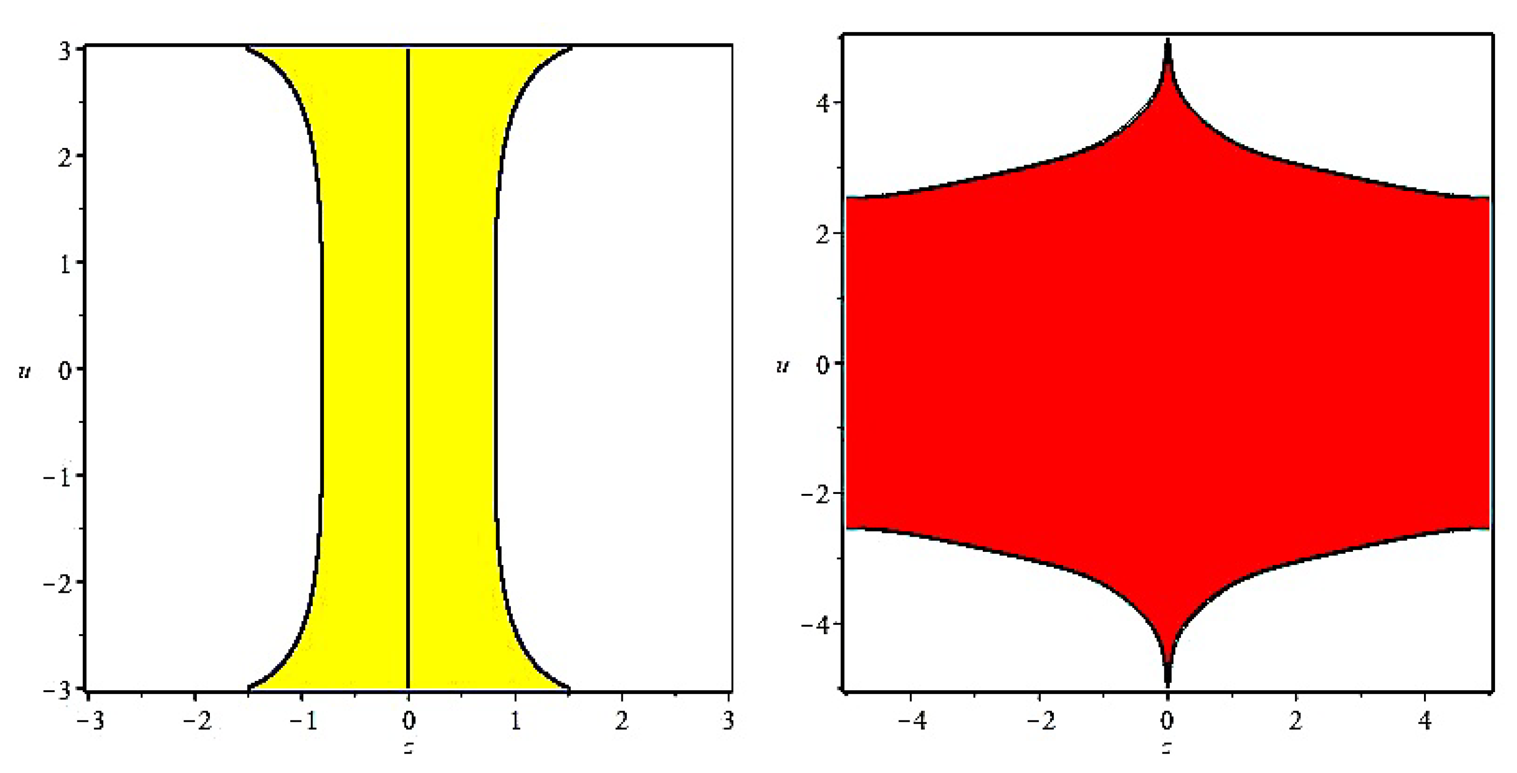
Since the stability matrix depends on two parameters z and u, we plot the stability regions in the (z, u)—plane for both k = 2 and k = 3 respectively, in Figure 1, where the colored regions (blue and green) are the stability regions corresponding to the test problem y = λ 2 y .
Since the Lambert-Watson test does not contain the first derivative, another usual test equation to analyze linear stability is the one given by
y = 2 λ y λ 2 y ,
which has bounded solutions for λ 0 that tend to zero when x . We have plotted in Figure 2 the corresponding stability region for the BFFM for k = 2 and k = 3 .

4. Implementation and Numerical Experiments

4.1. Implementation of BFFM

The BFFM is implemented using a written code in Maple 2016.1 enhanced by the feature f s o l v e for both linear nonlinear problems respectively. All numerical experiments are conducted on a Laptop with the following features
  • 64 bit Windows 10 Pro Operating System,
  • Intel (R) Celeron CPU N3060 @ 1.60 GHz processor, and
  • 4.00GB RAM memory.
The summary of how BFFM is applied to solve initial value problems (IVPs) with oscillatory solutions in a block by-block fashion is as follows:
Step 1: Choose N, h = ( x N x 0 ) / N to form the grid Γ N = { x 0 , x 1 , , x N } with x i = x 0 + i h . Note that N must be a multiple of k , N = m k .
Step 2: Using the difference Equation (13), n = 0 , solve for the values of ( y 1 , y 2 , , y k ) T and ( y 1 , y 2 , , y k ) T simultaneously on the block sub-interval [ x 0 , x k ] , as y 0 and y 0 are known from the IVP (1). As an illustration, we outline the procedure with k = 2 for the two first block intervals, when n = 0 and n = 2 , in Appendix D.
Step 3: Next, for n = k , the values of ( y k + 1 , y k + 2 , , y 2 k ) T and ( y k + 1 , y k + 2 , , y 2 k ) T are simultaneously obtained over the block sub-interval [ x k , x 2 k ] , as y k and y k are known from the previous block.
Step 4: The process is continued for 2 k , 3 k , , ( N 1 ) k to obtain the numerical solution to (1) on the sub-intervals [ x 0 , x k ] , [ x k , x 2 k ] , …, [ x N k , x N ] .

4.2. Numerical Examples

In order to examine the effectiveness of the BFFM derived in Section 2, we apply specifically BFFM for k = 2 on some well known oscillatory problems that were solved in the recent literature. The criteria used in the numerical investigations are two-fold, the accuracy and the efficiency. A measure of the accuracy is investigated using the maximum error of the approximate solution defined as E r r o r = max 1 n N y ( x ) y n , where y ( x ) is the exact solution and y n is the numerical solution obtained using BFFM while the computational efficiency can be observed through the plots of the maximum errors versus the number of function evaluations, NFE, required by each integrator. We emphasize that the fitting frequencies used in the numerical experiments have been obtained from the problems referenced from the literature.

4.3. Problems Where the First Derivative Appears Explicitly

4.3.1. Example 1

As our first test, we consider the following general second order IVP
y + ω 2 y = δ y ,
with initial conditions y ( 0 ) = 1 and y ( 0 ) = δ 2 , whose analytical solution is y ( x ) = e ( δ 2 ) x cos ( x ω 2 δ 2 4 ) .
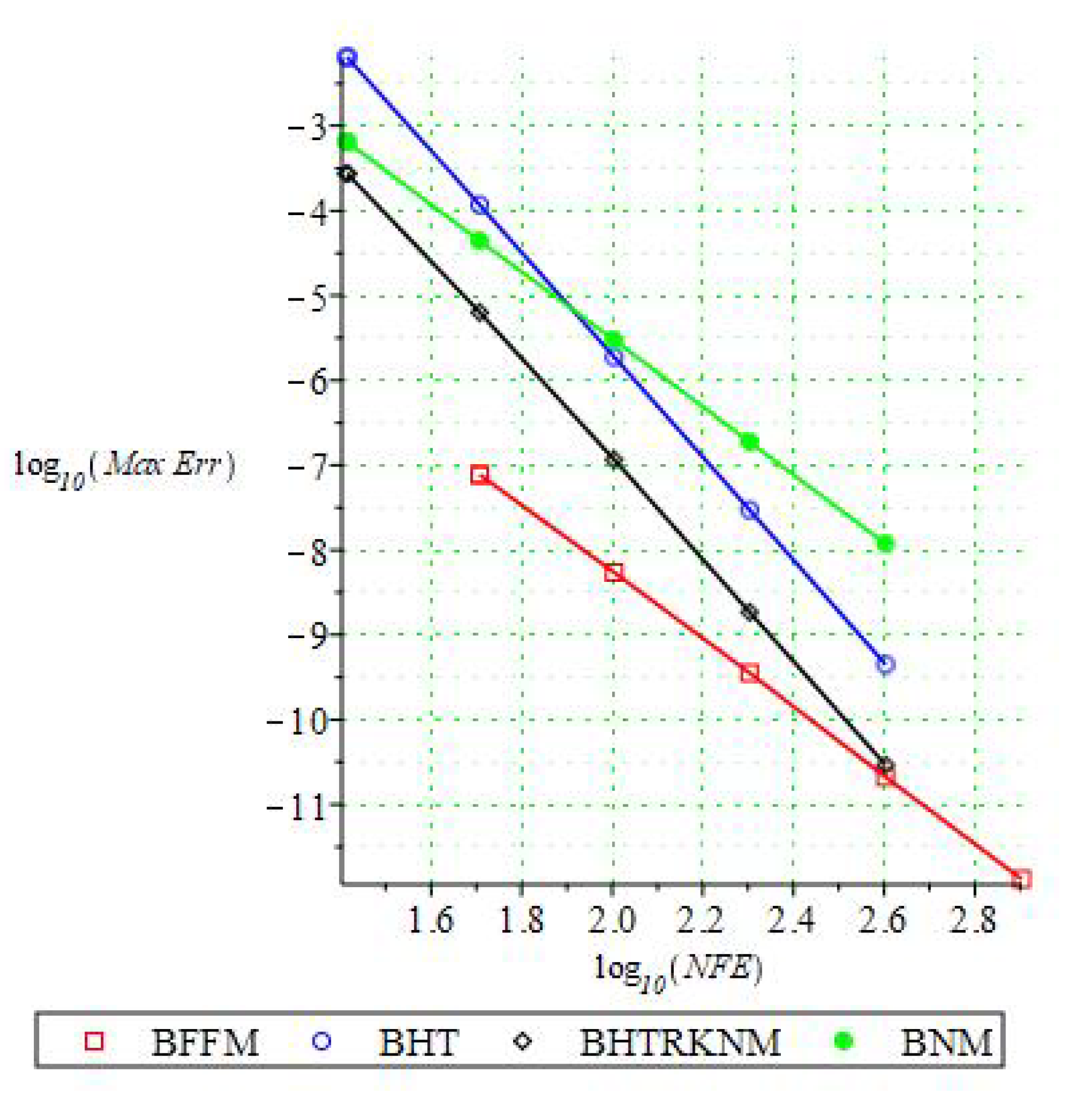
We solve this problem in the interval [0,100] with ω = 1 , δ = 10 3 and compare the result of BFFM with the BNM of order 5 in Jator and Oladejo [57], BHT of order 5 and BHTRKNM of order 3 in Ngwane and Jator [19,58]. Table 1 shows the Maximum errors and the NFE, while the efficiency curves are presented in Figure 3.

4.3.2. Example 2

Let us consider the following oscillatory system
[ y 1 y 2 ] + [ 13 12 12 13 ] [ y 1 ( x ) y 2 ( x ) ] = 12 ε 5 [ 3 2 2 3 ] [ y 1 y 2 ] + ε 2 [ f 1 ( x ) f 2 ( x ) ] ,
( y 1 ( 0 ) , y 2 ( 0 ) ) T = ( ε , ε ) T , ( y 1 ( 0 ) , y 2 ( 0 ) ) T = ( 4 , 6 ) T ,
with
[ f 1 ( x ) f 2 ( x ) ] = [ 36 5 sin ( x ) + 24 sin ( 5 x ) 24 5 sin ( x ) 36 sin ( 5 x ) ] ,
and whose solution in closed form is given as
[ y 1 ( x ) y 2 ( x ) ] = [ sin ( x ) sin ( 5 x ) + ε cos ( x ) sin ( x ) + sin ( 5 x ) + ε cos ( 5 x ) ] .
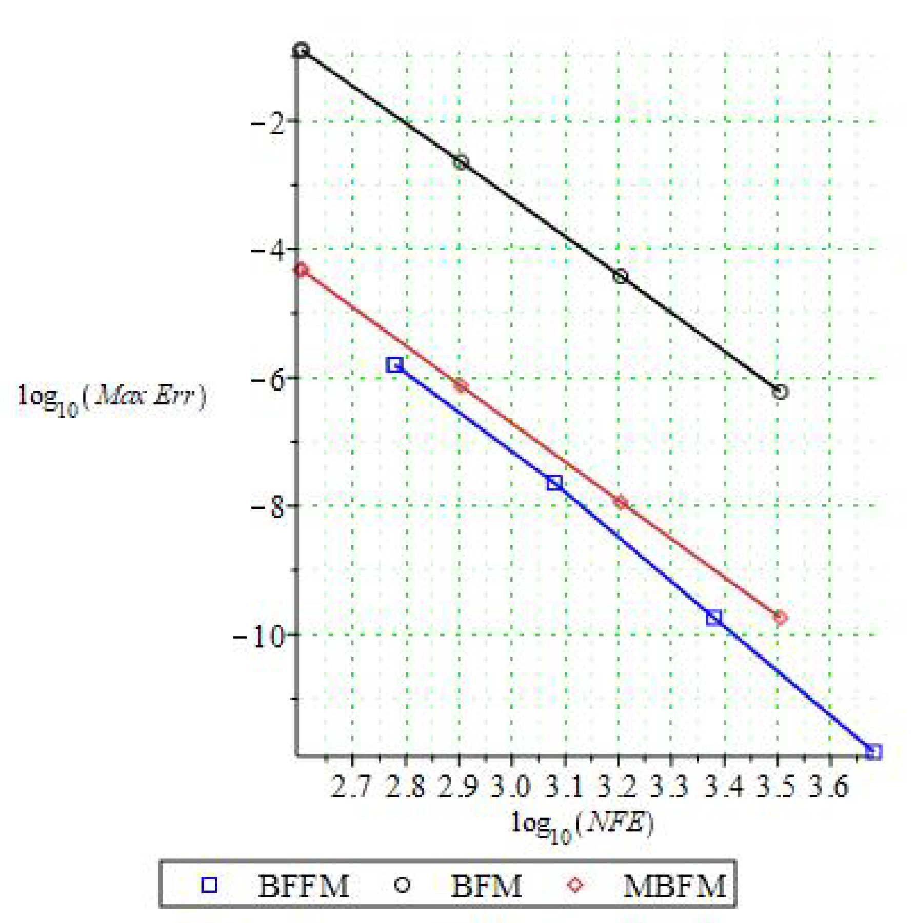
In our experiment, we choose the parameter value ε = 10 3 and the fitting frequency as ω = 5 . The problem is solved in the interval [0, 100]. The step sizes for the numerical experiment are taken as h = 1 2 i , i = 3 , 4 , 5 , 6 . The numerical results of BFFM in comparison with the Block Falkner methods (BFM) of order 5 in Ramos et al. [32] and Modified Block Falkner methods (MBFM) of order 5 in Ehigie and Okunuga [36] are displayed in Table 2 while the efficiency curves are displayed in Figure 4 respectively.

4.3.3. Example 3

Consider the popular Van der Pol equation given by
y + y = δ ( 1 y 2 ) y
with initial values
y ( 0 ) = 2 + 1 96 δ 2 + 1033 552960 δ 4 + 1019689 55738368000 δ 2 , y ( 0 ) = 0 .
This is a nonlinear scalar equation. In our numerical experiment, the parameter δ is selected as δ = 10 3 and the principal frequency is chosen as ω = 1 . We integrate this problem in the interval [0, 100]. In order to compare error of different methods, we use step lengths h = 1 2 i , i = 1 , 2 , 3 , 4 . We emphasize that the analytic solution of this problem does not exists, thus, we used a reference numerical solution which is obtained via special perturbation approach (Anderson and Geer [59] and Verhulst [60]). The BFFM results in comparison with the Block Falkner methods (BFM) of order 5 in Ramos et al. [32], Modified Block Falkner methods (MBFM) of order 5 in Ehigie and Okunuga [36] and The two-stage and three-stage Two-derivative Runge-Kutta-Nystrom Methods (TDRKN2 and TDRKN3) of orders 4 and 5 respectively in Chen et al. [25] are displayed in Table 3 while the efficiency curves are displayed in Figure 4 respectively. It is evident from the results in Table 3 and Figure 5 that BFFM performs better than some of the existing methods in the literature.

4.4. Problems Where the First Derivative Does Not Appear Explicitly

4.4.1. Example 4

As our fourth experiment, we consider the periodically forced nonlinear IVP
{ y + y 3 + y = ( cos ( x ) + ϵ sin ( 10 x ) ) 3 99 ϵ sin ( 10 x ) , y ( 0 ) = 1 , y ( 0 ) = 10 ϵ , 0 x 1000 ,
whose analytic solution is y ( x ) = cos ( x ) + ϵ sin ( 10 x ) . For this problem, ω = 1 is selected as principal frequency with parameter ϵ = 10 10 . Table 4 shows the performnce of BFFM in comparison with the TFARKN by Fang et al. [14], the EFRK by Franco [39] and the EFRKN by Franco [10] respectively. The efficiency curves of the BFFM and the other methods used for comparisons are displayed in Figure 6.

4.4.2. Example 5

As our fifth numerical experiment, we consider the following nonlinear system
[ y 1 y 2 ] + [ 13 12 12 13 ] [ y 1 ( x ) y 2 ( x ) ] = V y , y ( 0 ) = [ 1 1 ] , y ( 0 ) = [ 5 5 ] ,
with V ( y ) = y 1 y 2 ( y 1 + y 2 ) 3 , whose solution in closed form is given as
[ y 1 ( x ) y 2 ( x ) ] = [ sin ( 5 x ) cos ( 5 x ) sin ( 5 x ) + cos ( 5 x ) ] .
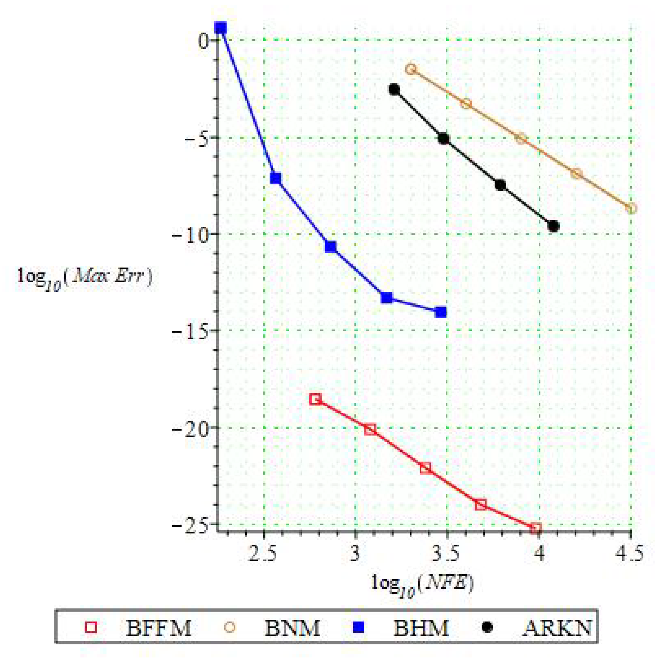
Table 5 and Figure 7 show the superiority of the BFFM in the interval [0, 100] over the BNM of order 5 in Jator and oladejo [57], the BHM of order 11 in Jator and King [61] and the fourth order ARKN in Franco [9].

4.4.3. Example 6

We consider the following well known two body problem
y 1 ( x ) = y 1 r 3 , y 1 ( 0 ) = 1 , y 1 ( 0 ) = 0
y 2 ( x ) = y 2 r 3 , y 2 ( 0 ) = 0 , y 2 ( 0 ) = 1 ,
where r = y 1 2 + y 2 2 , and the solution in closed form is given by y 1 ( x ) = cos ( x ) , y 2 ( x ) = sin ( x ) .
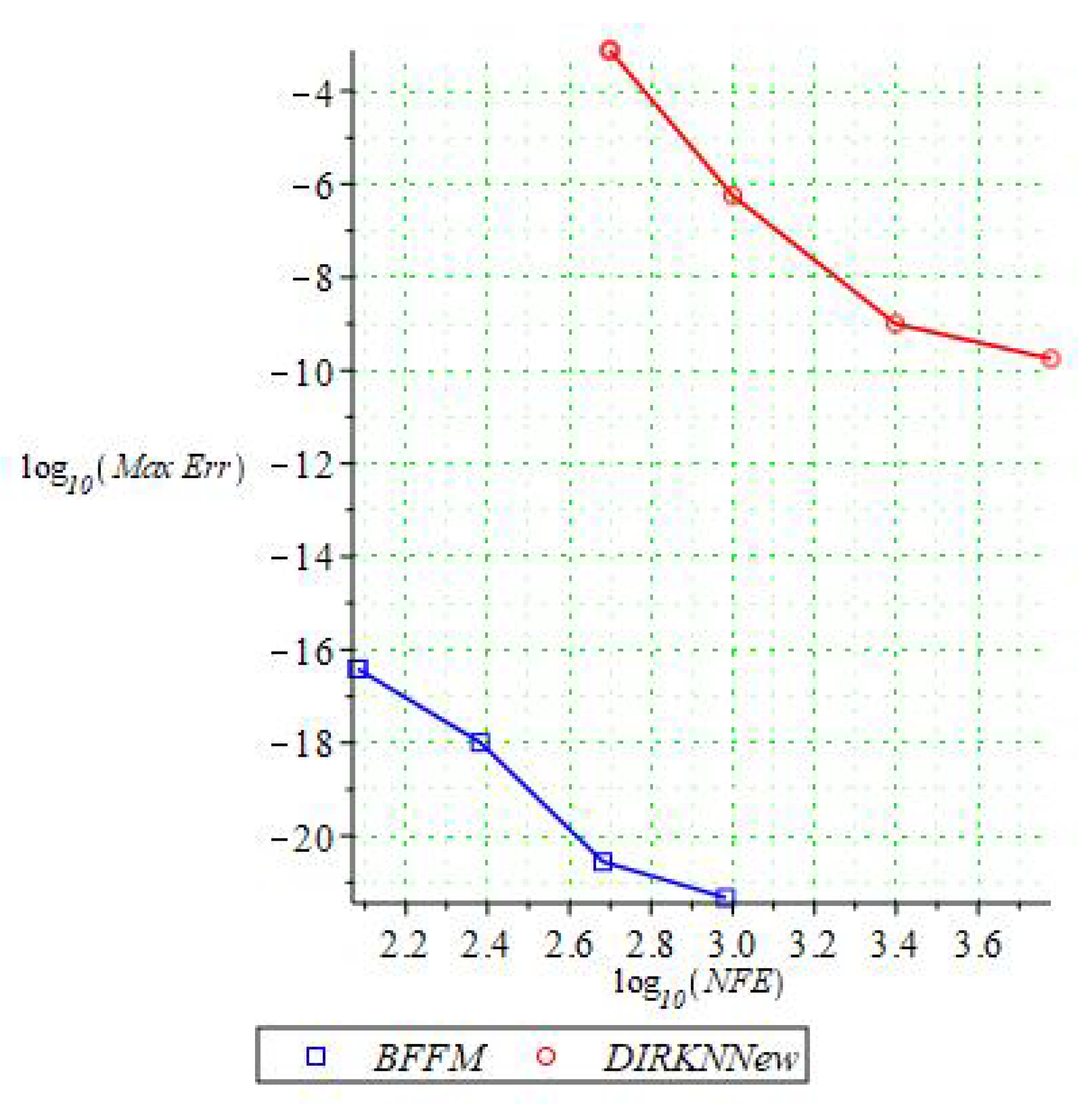
Table 6 reveals the performance of our proposed BFFM in the interval 0 x 10 with ω = 1 as it compared with the fourth order DIRKNNew of Senu et al. [15] while Figure 8 establishes the efficiency of BFFM.

5. Conclusions

In this paper, we have proposed a family of Adapted block Falkner methods using third derivative for solving second order initial value problem with oscillatory solution directly numerically. The methods are applied in block form as simultaneous numerical integrators and thus, do not suffer the disadvantages of predictor-corrector mode. The basic properties of the methods are investigated and discussed. The convergence of the proposed methods was established and the stability regions are presented. The numerical results on well-known second order initial value problems with oscillatory solutions show the effectiveness of the proposed methods compared with some existing methods in the reviewed literature. Although the proposed family of methods can be implemented with variable steps, that aspect was not considered in the current work, but will be considered in our future research.

Author Contributions

Writing—original draft, R.A. and R.O.; Writing—review–editing, H.R. and S.J. All authors have read and agreed to the published version of the manuscript.

Funding

This research did not receive any specific grant from funding agencies in the public, commercial, or not-for-profit sectors.

Institutional Review Board Statement

Not applicable.

Informed Consent Statement

Not applicable.

Data Availability Statement

Not applicable.

Conflicts of Interest

The authors declare no conflict of interest.

Appendix A. Specification of Entries of Matrix Π, the Determinant of Π and Determinants of Πi

Π = [ 1 x n + 1 sin ( ω x n + 1 ) cos ( ω x n + 1 ) sinh ( ω x n + 1 ) cosh ( ω x n + 1 ) 0 1 cos ( ω x n + 1 ) ω sin ( ω x n + 1 ) ω cosh ( ω x n + 1 ) ω sinh ( ω x n + 1 ) ω 0 0 ω 2 sin ( ω x n ) ω 2 cos ( ω x n ) ω 2 sinh ( ω x n ) cosh ( ω x n ) ω 2 0 0 ω 2 sin ( ω x n + 1 ) ω 2 cos ( ω x n + 1 ) ω 2 sinh ( ω x n + 1 ) cosh ( ω x n + 1 ) ω 2 0 0 ω 2 sin ( ω x n + 2 ) ω 2 cos ( ω x n + 2 ) ω 2 sinh ( ω x n + 2 ) cosh ( ω x n + 2 ) ω 2 0 0 ω 3 cos ( ω x n + 2 ) ω 3 sin ( ω x n + 2 ) ω 3 cosh ( ω x n + 2 ) sinh ( ω x n + 2 ) ω 3 ]
d e t ( Π ) = ω 9 ( cos ( ω h ) sinh ( 2 ω h ) + sin ( ω h ) cosh ( 2 ω h ) sin ( 2 ω h ) cosh ( ω h ) + cos ( 2 ω h ) sinh ( ω h ) + sin ( ω h ) + sinh ( ω h ) )
d e t ( Π 0 ) = 2 ( ( cos ( ω h ) ω f n + 1 x n + 1 + ( ( y n + 1 x n + 1 y n + 1 ) ω 2 f n + 1 ) sin ( ω h ) ) ( cosh ( ω h ) ) 2 + ( ( cos ( ω h ) ) 2 ω f n + 1 x n + 1 + ( ( ( y n + 1 x n + 1 + y n + 1 ) ω 2 + f n + 1 ) sinh ( ω h ) ( ( y n + 1 x n + 1 y n + 1 ) ω 2 + f n + 1 ) sin ( ω h ) ) cos ( ω h ) x n + 1 ( sin ( ω h ) ω f n + 1 + g n + 2 sinh ( ω h ) + ( g n + 2 x n + 1 + f n + f n + 2 ) sin ( ω h ) ω x n + 1 ( f n + 1 1 / 2 f n + 2 ) cosh ( ω h ) + ( ( ( y n + 1 x n + 1 y n + 1 ) ω 2 + f n + 1 ) sinh ( ω h ) ω f n + 2 x n + 1 ) ( cos ( ω h ) ) 2 + ( ( sin ( ω h ) ω f n + 1 x n + 1 + g n + 2 x n + 1 f n f n + 2 ) sinh ( ω h ) + x n + 1 ( sin ( ω h ) g n + 2 + ω f n + 1 ) cos ( ω h ) + ω x n + 1 ( sin ( ω h ) ( f n + f n + 2 ) sinh ( ω h ) + 1 / 2 f n + 2 ) ω 7
d e t ( Π 1 ) = ω 7 ( ω ( y n + 1 sin ( ω h ) ω cos ( ω h ) f n + 1 + f n + 2 ) cosh ( 2 ω h ) + ( ω 2 y n + 1 cos ( ω h ) sin ( ω h ) ω f n + 1 g n + 2 ) sinh ( 2 ω h ) + ω ( ω y n + 1 sinh ( ω h ) + cosh ( ω h ) f n + 1 f n + 2 ) cos ( 2 ω h ) + ( cosh ( ω h ) ω 2 y n + 1 ω f n + 1 sinh ( ω h ) + g n + 2 ) sin ( 2 ω h ) + ( 2 ω ( f n + f n + 2 ) sin ( ω h ) + ω 2 y n + 1 + 2 cos ( ω h ) g n + 2 ) sinh ( ω h ) + ( ω 2 y n + 1 2 cosh ( ω h ) g n + 2 ) sin ( ω h ) ω f n + 1 ( cosh ( ω h ) cos ( ω h ) )
d e t ( Π 2 ) = ω 6 ( ω ( cos ( ω x n + 1 ) f n + 2 cos ( ω x n + 2 ) f n + 1 ) cosh ( 2 ω h ) + ( ω sin ( ω x n + 2 ) f n + 1 + g n + 2 cos ( ω x n + 1 ) ) sinh ( 2 ω h ) + ( cos ( ω x n + 2 ) g n + 2 ω ( f n + f n + 2 ) sin ( ω x n + 2 ) g n + 2 cos ( ω x n ) sinh ( ω h ) + ω ( cos ( ω x n + 1 ) f n cosh ( ω h ) f n cos ( ω x n + 2 ) + cos ( ω x n ) ( cosh ( ω h ) f n + 2 f n + 1 )
d e t ( Π 3 ) = ω 6 ( ω ( sin ( ω x n + 1 ) f n + 2 sin ( ω x n + 2 ) f n + 1 ) cosh ( 2 ω h ) + ( ω ( f n f n + 1 + f n + 2 ) cos ( ω x n + 2 ) g n + 2 ( sin ( ω x n ) sin ( ω x n + 1 ) + sin ω x n + 2 sinh ( ω h ) + ( sin ( ω x n + 1 ) f n cosh ( ω h ) f n sin ω x n + 2 ) + sin ( ω x n ) cosh ( ω h ) f n + 2 f n + 1 ω
d e t ( Π 4 ) = ω 6 ( ω ( cosh ( ω x n + 1 ) f n + 2 cosh ( ω x n + 2 ) f n + 1 ) cos ( 2 ω h ) + ( ω sinh ( ω x n + 2 ) f n + 1 + g n + 2 cosh ( ω x n + 1 ) ) sin ( 2 ω h ) + ( cosh ( ω x n + 2 ) g n + 2 + ω ( f n + f n + 2 ) sinh ( ω x n + 2 ) g n + 2 cosh ( ω x n ) sin ( ω h ) + ω ( cosh ( ω x n + 1 ) f n cos ( ω h ) f n cosh ( ω x n + 2 ) + cosh ( ω x n ) ( cos ( ω h f n + 2 f n + 1 ) )
d e t ( Π 5 ) = ω 6 ( ω ( sinh ( ω x n + 1 ) f n + 2 sinh ( ω x n + 2 ) f n + 1 ) cos ( 2 ω h ) + ( ω f n + 1 cosh ( ω x n + 2 ) + sinh ( ω x n + 1 ) g n + 2 ) sin ( 2 ω h ) + ( ω ( f n + f n + 2 ) cosh ( ω x n + 2 ) g n + 2 ( sinh ( ω x n ) + sinh ( ω x n + 2 ) ) sin ( ω h ) + ( sinh ( ω x n + 1 ) f n cos ( ω h ) f n sinh ( ω x n + 2 ) + sinh ( ω x n ) ( cos ( ω h f n + 2 f n + 1 ) ) ω ,

Appendix B. Coefficients of the Main Methods of the BFFM for k = 2

β 20 = 2 ( u sin ( u ) + cos ( u ) 1 ) sinh ( u ) sin ( u ) ( cosh ( u ) 1 ) ψ 1 ( u ) = 1 80 17 u 4 1209600 68953 u 8 435891456000 6136859 u 12 14938871980032000 β 21 = 1 ψ 1 ( u ) ( ( u sin ( u ) + cos ( u ) 2 ) sinh ( 2 u ) + ( u sinh ( u ) cosh ( u ) + 2 ) sin ( 2 u ) ) + ( cos ( u ) u sin ( u ) ) cosh ( 2 u ) + ( cosh ( u ) u + sinh ( u ) ) cos ( 2 u ) cos ( u ) u + cosh ( u ) u sin ( u ) + sinh ( u ) ) = 3 10 + 271 u 4 151200 + 277219 u 8 54486432000 + 50922197 u 12 1867358997504000 β 22 = 1 ψ 1 ( u ) ( ( u + sin ( u ) ) cosh ( 2 u ) + ( u sinh ( u ) ) cos ( 2 u ) + cos ( u ) sinh ( 2 u ) ) sin ( 2 u ) cosh ( u ) + ( 2 u sin ( u ) 2 cos ( u ) + 1 ) sinh ( u ) + sin ( u ) ( 2 cosh ( u ) 1 ) ) = 17 80 + 403 u 4 403200 + 1815161 u 8 435891456000 + 265892323 u 12 14938871980032000 γ 2 = ( u 2 sin ( u ) ) sinh ( 2 u ) + ( u + 2 sinh ( u ) ) sin ( 2 u ) 2 u ( cos ( u ) sinh ( u ) sin ( u ) cosh ( u ) ) u ψ 1 ( u ) = 17 80 + 403 u 4 403200 + 1815161 u 8 435891456000 + 265892323 u 12 14938871980032000 ,
where
ψ 1 ( u ) = u 2 cos ( u ) sinh ( 2 u ) u 2 sin ( u ) cosh ( 2 u ) + u 2 sin ( 2 u ) cosh ( u ) u 2 cos ( 2 u ) sinh ( u ) u 2 sin ( u ) u 2 sinh ( u )
β ¯ 20 = 2 sin ( u ) sinh ( u ) + cos ( u ) cosh ( u ) ψ 2 ( u ) = 1 / 48 u 4 34560 367 u 8 1341204480 44591 u 12 58583811686400 β ¯ 21 = cosh ( 2 u ) cos ( u ) + sinh ( 2 u ) sin ( u ) cos ( 2 u ) cosh ( u ) + sin ( 2 u ) sinh ( u ) 2 cosh ( 2 u ) + 2 cos ( 2 u ) cos ( u ) + cosh ( u ) ψ 2 ( u ) = 5 12 + 37 u 4 12096 + 625 u 8 67060224 + 141389 u 12 2929190584320 β ¯ 22 = 2 cosh ( 2 u ) cos ( u ) + 2 cos ( 2 u ) cosh ( u ) + 2 sin ( u ) sinh ( u ) + cosh ( 2 u ) + cos ( 2 u ) ψ 2 ( u ) = 29 48 + 443 u 4 241920 + 913 u 8 121927680 + 1867219 u 12 58583811686400 γ ¯ 2 = ( cos ( u ) 1 ) sinh ( 2 u ) + ( cosh ( u ) + 1 ) sin ( 2 u ) + sin ( u ) cosh ( 2 u ) cos ( 2 u ) sinh ( u ) + ( 2 cos ( u ) 1 ) sinh ( u ) + ( 2 cosh ( u ) + 1 ) sin ( u ) u ψ 2 ( u ) = 1 / 8 19 u 4 40320 2207 u 8 1117670400 81083 u 12 9763968614400
where
ψ 2 ( u ) = u sin ( u ) + u cos ( 2 u ) sinh ( u ) u sin ( 2 u ) cosh ( u ) u cos ( u ) sinh ( 2 u ) + u sin ( u ) cosh ( 2 u ) + u sinh ( u )

Appendix C. Matrices RA1A0 for k = 2 and k = 3

[ R A 1 A 0 ] k = 2 = [ 0 R 1 0 R R R 0 R 0 0 0 R 1 0 0 R R ] ,
[ R A 1 A 0 ] k = 3 = [ 0 0 R 1 0 0 R 0 R R 0 0 R R 0 R 0 0 2 R 0 0 0 0 0 R 1 0 0 0 0 R R 0 0 0 R 0 R ] .

Appendix D. Illustration of Step 2 of the Implementation for k = 2 When n = 0 and n = 2

For k = 2 , when n = 0 , the Equation (13) becomes
A 1 Y 1 = A 0 Y 0 + h 2 B 0 F 0 + h 2 B 1 F 1 ,
where
Y 1 = ( y 1 , y 2 , h y 1 , h y 2 ) T ,
Y 0 = ( y 1 , y 0 , h y 1 , h y 0 ) T ,
F 1 = ( f 1 , f 2 , h g 1 , h g 2 ) T ,
F 0 = ( f 1 , f 0 , h g 1 , h g 0 ) T
Substituting for the square matrices A 0 , A 1 , B 0 and B 1 in Equation (A3) to obtain
{ y 2 h y 2 = y 0 + h 2 j = 0 2 ( β 2 j 0 ( u ) y j + h γ 2 0 ( u ) y 2 ) y 1 + y 2 + h y 2 = h 2 j = 0 2 ( β 2 j ( u ) y j + h γ 2 ( u ) y 2 ) h y 1 = h y 0 + h 2 j = 0 2 ( β ¯ 2 j 0 y j ( u ) + h γ ¯ 2 0 ( u ) y 2 ) h y 1 + h y 2 = h 2 j = 0 2 ( β ¯ 2 j y j ( u ) + h γ ¯ 2 ( u ) y 2 ) .
We solve Equation (A4) simultaneously to obtain the values of ( y 1 , y 2 , y 1 , y 2 ) T on the block sub-interval [ x 0 , x 2 ] , as y 0 and y 0 are known from the IVP (1), y = f ( x , y , y ) and y is the derivative of y .
When n = 2 , the Equation (13) becomes
A 1 Y 3 = A 0 Y 2 + h 2 B 0 F 2 + h 2 B 1 F 3 ,
where
Y 3 = ( y 3 , y 4 , h y 3 , h y 4 ) T ,
Y 2 = ( y 1 , y 2 , h y 1 , h y 2 ) T ,
F 3 = ( f 3 , f 4 , h g 3 , h g 4 ) T ,
F 2 = ( f 1 , f 2 , h g 1 , h g 2 ) T
We then substitute for the square matrices A 0 , A 1 , B 0 and B 1 in Equation (A5) to obtain
{ y 4 h y 4 = y 2 + h 2 j = 0 2 ( β 2 j 0 ( u ) y j + 2 + h γ 2 0 ( u ) y 4 ) y 3 + y 4 + h y 4 = h 2 j = 0 2 ( β 2 j ( u ) y j + 2 + h γ 2 ( u ) y 4 ) h y 3 = h y 1 + h 2 j = 0 2 ( β ¯ 2 j 0 y j + 2 ( u ) + h γ ¯ 2 0 ( u ) y 4 ) h y 3 + h y 4 = h 2 j = 0 2 ( β ¯ 2 j y j + 2 ( u ) + h γ ¯ 2 ( u ) y 4 ) .
We solve Equation (A6) simultaneously to obtain the values of ( y 3 , y 4 , y 3 , y 4 ) T on the block sub-interval [ x 2 , x 4 ] , as y 2 and y 2 are known from the previous block.

References

  1. Lambert, J.D.; Watson, I.A. Symmetric multistip methods for periodic initial value problems. IMA J. Appl. Math. 1976, 18, 189–202. [Google Scholar] [CrossRef]
  2. Anantha Krishnaiah, U. P-stable Obrechkoff methods with minimal phase-lag for periodic initial value problems. Math. Comput. 1987, 49, 553–559. [Google Scholar] [CrossRef] [Green Version]
  3. Simos, T. Dissipative trigonometrically-fitted methods for second order IVPs with oscillating solution. Int. J. Mod. Phys. C 2002, 13, 1333–1345. [Google Scholar] [CrossRef]
  4. Hairer, E.; Nørsett, S.P.; Wanner, G. Solving Ordinary Differential Equations I. Nonstiff Problems; Springer: Berlin, Germany, 1993. [Google Scholar]
  5. Tsitouras, C. Explicit eighth order two-step methods with nine stages for integrating oscillatory problems. Int. J. Mod. Phys. C 2006, 17, 861–876. [Google Scholar] [CrossRef]
  6. Tsitouras, C.; Simos, T. Trigonometric-fitted explicit numerov-type method with vanishing phase-lag and its first and second derivatives. Mediterr. J. Math. 2018, 15, 168. [Google Scholar] [CrossRef]
  7. Wang, B.; Liu, K.; Wu, X. A Filon-type Asymptotic Approach to Solving Highly Oscillatory Second-Order Initial Value Problems. J. Comput. Phys. 2013, 243, 210–223. [Google Scholar] [CrossRef]
  8. Li, J.; Wang, B.; You, X.; Wu, X. Two-step extended RKN methods for oscillatory systems. Comput. Phys. Commun. 2011, 182, 2486–2507. [Google Scholar] [CrossRef]
  9. Franco, J. New methods for oscillatory systems based on ARKN methods. Appl. Numer. Math. 2006, 56, 1040–1053. [Google Scholar] [CrossRef]
  10. Franco, J. Runge–Kutta methods adapted to the numerical integration of oscillatory problems. Appl. Numer. Math. 2004, 50, 427–443. [Google Scholar] [CrossRef]
  11. Ramos, H.; Patricio, M. Some new implicit two-step multiderivative methods for solving special second-order IVP’s. Appl. Math. Comput. 2014, 239, 227–241. [Google Scholar] [CrossRef]
  12. Chen, Z.; You, X.; Shi, W.; Liu, Z. Symmetric and symplectic ERKN methods for oscillatory Hamiltonian systems. Comput. Phys. Commun. 2012, 183, 86–98. [Google Scholar] [CrossRef]
  13. Shi, W.; Wu, X. On symplectic and symmetric ARKN methods. Comput. Phys. Commun. 2012, 183, 1250–1258. [Google Scholar] [CrossRef]
  14. Fang, Y.; Song, Y.; Wu, X. A robust trigonometrically fitted embedded pair for perturbed oscillators. J. Comput. Appl. Math. 2009, 225, 347–355. [Google Scholar] [CrossRef] [Green Version]
  15. Senu, N.; Suleiman, M.; Ismail, F.; Othman, M. A new diagonally implicit Runge-Kutta-Nyström method for periodic IVPs. WSEAS Trans. Math. 2010, 9, 679–688. [Google Scholar] [CrossRef]
  16. Guo, B.Y.; Yan, J.P. Legendre–Gauss collocation method for initial value problems of second order ordinary differential equations. Appl. Numer. Math. 2009, 59, 1386–1408. [Google Scholar] [CrossRef]
  17. Vigo-Aguiar, J.; Ramos, H. Variable stepsize implementation of multistep methods for y″ = f(x,y,y′). J. Comput. Appl. Math. 2006, 192, 114–131. [Google Scholar] [CrossRef] [Green Version]
  18. Jator, S.N. Implicit third derivative Runge-Kutta-Nyström method with trigonometric coefficients. Numer. Algorithms 2015, 70, 133–150. [Google Scholar] [CrossRef]
  19. Ngwane, F.; Jator, S. A trigonometrically fitted block method for solving oscillatory second-order initial value problems and Hamiltonian systems. Int. J. Differ. Equ. 2017, 2017, 9293530. [Google Scholar] [CrossRef]
  20. Mahmoud, S.; Osman, M.S. On a class of spline-collocation methods for solving second-order initial-value problems. Int. J. Comput. Math. 2009, 86, 616–630. [Google Scholar] [CrossRef]
  21. Awoyemi, D. A new sixth-order algorithm for general second order ordinary differential equations. Int. J. Comput. Math. 2001, 77, 117–124. [Google Scholar] [CrossRef]
  22. Liu, K.; Wu, X. Multidimensional ARKN methods for general oscillatory second-order initial value problems. Comput. Phys. Commun. 2014, 185, 1999–2007. [Google Scholar] [CrossRef]
  23. You, X.; Zhang, R.; Huang, T.; Fang, Y. Symmetric collocation ERKN methods for general second-order oscillators. Calcolo 2019, 56, 52. [Google Scholar] [CrossRef]
  24. Li, J.; Lu, M.; Qi, X. Trigonometrically fitted multi-step hybrid methods for oscillatory special second-order initial value problems. Int. J. Comput. Math. 2018, 95, 979–997. [Google Scholar] [CrossRef]
  25. Chen, Z.; Qiu, Z.; Li, J.; You, X. Two-derivative Runge-Kutta-Nyström methods for second-order ordinary differential equations. Numer. Algorithms 2015, 70, 897–927. [Google Scholar] [CrossRef]
  26. Li, J.; Wang, X.; Lu, M. A class of linear multi-step method adapted to general oscillatory second-order initial value problems. J. Appl. Math. Comput. 2018, 56, 561–591. [Google Scholar] [CrossRef]
  27. You, X.; Zhao, J.; Yang, H.; Fang, Y.; Wu, X. Order conditions for RKN methods solving general second-order oscillatory systems. Numer. Algorithms 2014, 66, 147–176. [Google Scholar] [CrossRef]
  28. Falkner, V.L. A method of numerical solution of differential equations. Lond. Edinb. Dublin Philos. Mag. J. Sci. 1936, 21, 624–640. [Google Scholar] [CrossRef]
  29. Collatz, L. The Numerical Treatment of Differential Equations; Springer Science & Business Media: Berlin, Germany, 2012; Volume 60. [Google Scholar]
  30. Ramos, H.; Mehta, S.; Vigo-Aguiar, J. A unified approach for the development of k-step block Falkner-type methods for solving general second-order initial-value problems in ODEs. J. Comput. Appl. Math. 2017, 318, 550–564. [Google Scholar] [CrossRef]
  31. Ramos, H.; Lorenzo, C. Review of explicit Falkner methods and its modifications for solving special second-order IVPs. Comput. Phys. Commun. 2010, 181, 1833–1841. [Google Scholar] [CrossRef]
  32. Ramos, H.; Singh, G.; Kanwar, V.; Bhatia, S. An efficient variable step-size rational Falkner-type method for solving the special second-order IVP. Appl. Math. Comput. 2016, 291, 39–51. [Google Scholar] [CrossRef]
  33. Ramos, H.; Rufai, M.A. Third derivative modification of k-step block Falkner methods for the numerical solution of second order initial-value problems. Appl. Math. Comput. 2018, 333, 231–245. [Google Scholar] [CrossRef]
  34. Li, J.; Wu, X. Adapted Falkner-type methods solving oscillatory second-order differential equations. Numer. Algorithms 2013, 62, 355–381. [Google Scholar] [CrossRef]
  35. Li, J. A family of improved Falkner-type methods for oscillatory systems. Appl. Math. Comput. 2017, 293, 345–357. [Google Scholar] [CrossRef]
  36. Ehigie, J.; Okunuga, S. A new collocation formulation for the block Falkner-type methods with trigonometric coefficients for oscillatory second order ordinary differential equations. Afr. Mat. 2018, 29, 531–555. [Google Scholar] [CrossRef]
  37. Gautschi, W. Numerical integration of ordinary differential equations based on trigonometric polynomials. Numer. Math. 1961, 3, 381–397. [Google Scholar] [CrossRef]
  38. Lyche, T. Chebyshevian multistep methods for ordinary differential equations. Numer. Math. 1972, 19, 65–75. [Google Scholar] [CrossRef]
  39. Franco, J. An embedded pair of exponentially fitted explicit Runge–Kutta methods. J. Comput. Appl. Math. 2002, 149, 407–414. [Google Scholar] [CrossRef] [Green Version]
  40. Franco, J. Exponentially fitted explicit Runge–Kutta–Nyström methods. J. Comput. Appl. Math. 2004, 167, 1–19. [Google Scholar] [CrossRef] [Green Version]
  41. Ixaru, L.G.; Berghe, G.V.; De Meyer, H. Frequency evaluation in exponential fitting multistep algorithms for ODEs. J. Comput. Appl. Math. 2002, 140, 423–434. [Google Scholar] [CrossRef] [Green Version]
  42. Berghe, G.V.; Van Daele, M. Exponentially-fitted Numerov methods. J. Comput. Appl. Math. 2007, 200, 140–153. [Google Scholar] [CrossRef] [Green Version]
  43. Jator, S.N.; Swindell, S.; French, R. Trigonometrically fitted block Numerov type method for y″ = f(x,y,y′). Numer. Algorithms 2013, 62, 13–26. [Google Scholar] [CrossRef]
  44. Jator, S. Block third derivative method based on trigonometric polynomials for periodic initial-value problems. Afr. Mat. 2016, 27, 365–377. [Google Scholar] [CrossRef]
  45. Ramos, H.; Vigo-Aguiar, J. On the frequency choice in trigonometrically fitted methods. Appl. Math. Lett. 2010, 23, 1378–1381. [Google Scholar] [CrossRef] [Green Version]
  46. Vigo-Aguiar, J.; Ramos, H. On the choice of the frequency in trigonometrically-fitted methods for periodic problems. J. Comput. Appl. Math. 2015, 277, 94–105. [Google Scholar] [CrossRef]
  47. Ramos, H.; Vigo-Aguiar, J. Variable-stepsize Chebyshev-type methods for the integration of second-order IVP’s. J. Comput. Appl. Math. 2007, 204, 102–113. [Google Scholar] [CrossRef] [Green Version]
  48. Coleman, J.P.; Duxbury, S.C. Mixed collocation methods for y″ = f(x,y). J. Comput. Appl. Math. 2000, 126, 47–75. [Google Scholar] [CrossRef] [Green Version]
  49. Coleman, J.P.; Ixaru, L.G. P-stability and exponential-fitting methods for y″ = f(x,y). IMA J. Numer. Anal. 1996, 16, 179–199. [Google Scholar] [CrossRef]
  50. Nguyen, H.S.; Sidje, R.B.; Cong, N.H. Analysis of trigonometric implicit Runge–Kutta methods. J. Comput. Appl. Math. 2007, 198, 187–207. [Google Scholar] [CrossRef] [Green Version]
  51. Ozawa, K. A functionally fitted three-stage explicit singly diagonally implicit Runge-Kutta method. Jpn. J. Ind. Appl. Math. 2005, 22, 403–427. [Google Scholar] [CrossRef]
  52. Franco, J.; Gómez, I. Trigonometrically fitted nonlinear two-step methods for solving second order oscillatory IVPs. Appl. Math. Comput. 2014, 232, 643–657. [Google Scholar] [CrossRef]
  53. Wu, J.; Tian, H. Functionally-fitted block methods for ordinary differential equations. J. Comput. Appl. Math. 2014, 271, 356–368. [Google Scholar] [CrossRef]
  54. Lambert, J.D. Computational Methods in Ordinary Differential Equations; Wiley: Hoboken, NJ, USA, 1973. [Google Scholar]
  55. Simeon, O.F. Numerical Methods for Initial Value Problems in Ordinary Differential Equations; Academic Press: Cambridge, UK, 1988. [Google Scholar]
  56. Ola Fatunla, S. Block methods for second order ODEs. Int. J. Comput. Math. 1991, 41, 55–63. [Google Scholar] [CrossRef]
  57. Jator, S.; Oladejo, H. Block Nyström method for singular differential equations of the Lane–Emden type and problems with highly oscillatory solutions. Int. J. Appl. Comput. Math. 2017, 3, 1385–1402. [Google Scholar] [CrossRef]
  58. Ngwane, F.; Jator, S. Solving the telegraph and oscillatory differential equations by a block hybrid trigonometrically fitted algorithm. Int. J. Differ. Equ. 2015, 2015. [Google Scholar] [CrossRef]
  59. Andersen, C.; Geer, J.F. Power series expansions for the frequency and period of the limit cycle of the van der Pol equation. SIAM J. Appl. Math. 1982, 42, 678–693. [Google Scholar] [CrossRef]
  60. Vehrulst, F. Nonlinear Differential Equations and Dynamical Systems, Universitext; Springer: Berlin/Heidelberg, Germany, 1996. [Google Scholar]
  61. Jator, S.N.; King, K.L. Integrating oscillatory general second-order initial value Problems using a block hybrid method of order 11. Math. Probl. Eng. 2018, 2018, 3750274. [Google Scholar] [CrossRef]
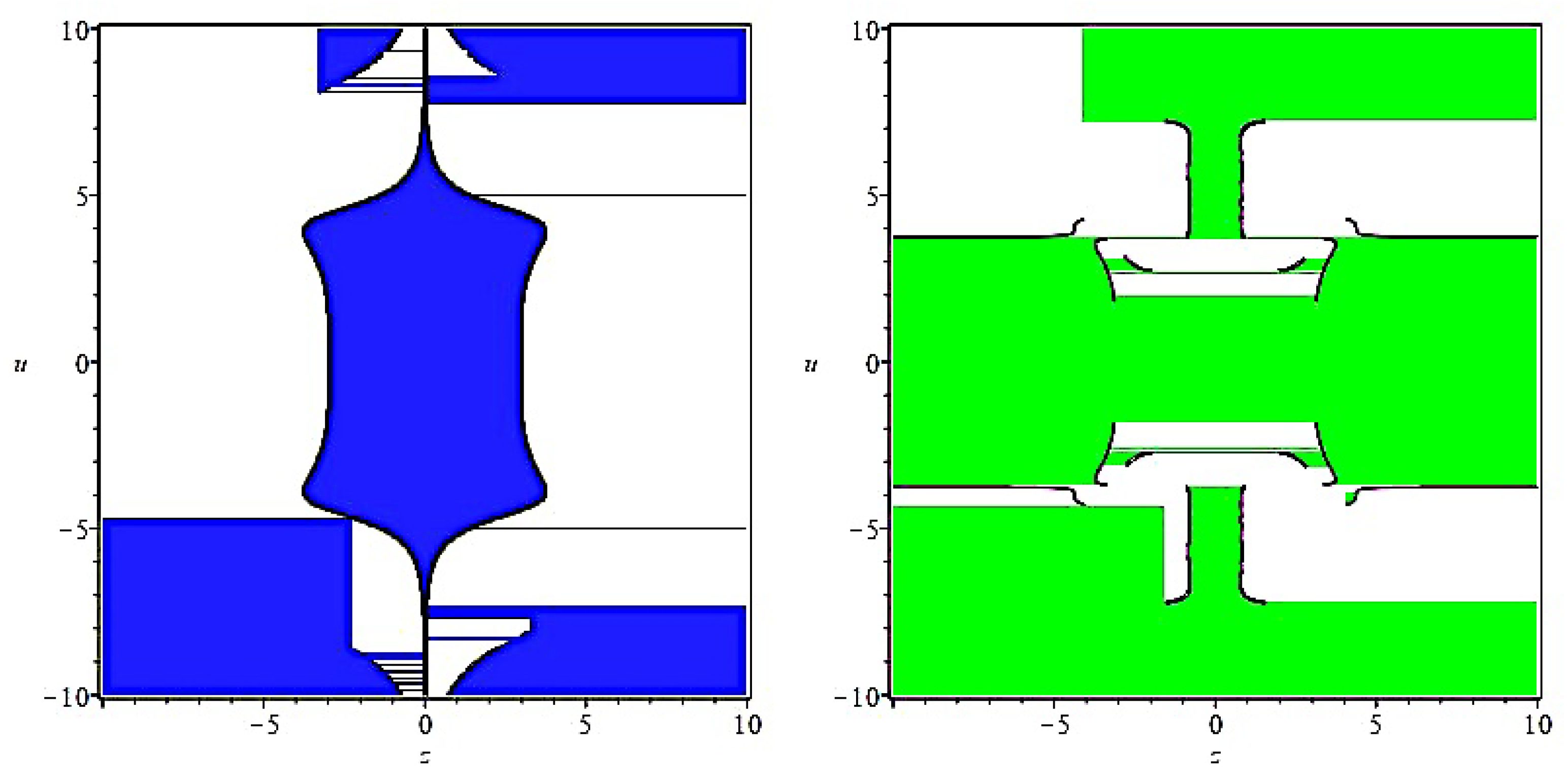
Figure 1. z u stability region of BFFM for k = 2 (left) and k = 3 (right) for the Lambert-Watson test.
Mathematics 09 00713 g001
Figure 2. z u stability region of BFFM for k = 2 (left) and k = 3 (right) for the test Equation (16).
Mathematics 09 00713 g002
Figure 3. Efficiency Curves for Example 1.
Mathematics 09 00713 g003
Figure 4. Efficiency Curves for Example 2.
Mathematics 09 00713 g004
Figure 5. Efficiency Curves for Example 3.
Mathematics 09 00713 g005
Figure 6. Efficiency Curves for Example 4.
Mathematics 09 00713 g006
Figure 7. Efficiency Curves for Example 5.
Mathematics 09 00713 g007
Figure 8. Efficiency Curves for Example 6.
Mathematics 09 00713 g008
Table 1. Data for Example 1 with ω = 1 , δ = 10 3 .
hBFFMBHTBHTRKNMBNM
ErrorNFEErrorNFEErrorNFEErrorNFE
2 7.71 × 10 8 51 2.74 × 10 4 26 6.48 × 10 4 26 6.46 × 10 3 26
1 5.43 × 10 9 101 6.34 × 10 6 51 4.39 × 10 5 51 1.17 × 10 4 51
1 2 3.55 × 10 10 201 1.16 × 10 7 101 2.99 × 10 6 101 1.88 × 10 6 101
1 4 2.11 × 10 11 401 1.85 × 10 9 201 1.88 × 10 7 201 2.96 × 10 8 201
1 8 1.32 × 10 12 801 2.92 × 10 11 401 1.18 × 10 8 401 4.46 × 10 10 401
Table 2. Data for Example 2 with ω = 5 , ε = 10 3 .
hBFFMBFMMBFM
ErrorNFEErrorNFEErrorNFE
1 8 0.75 × 10 6 601 1.26 × 10 1 401 4.79 × 10 5 401
1 16 2.29 × 10 8 1201 2.29 × 10 3 801 7.41 × 10 7 801
1 32 1.82 × 10 10 2401 3.80 × 10 5 1601 1.15 × 10 8 1601
1 64 1.48 × 10 12 4801 6.03 × 10 7 3201 1.82 × 10 10 3201
Table 3. Data for Example 3 with ω = 1 , δ = 10 3 .
hBFFMBFMMBFMTDRKN2TDRKN3
ErrorNFEErrorNFEErrorNFEErrorNFEErrorNFE
1 2 7.41 × 10 7 151 1.38 × 10 2 101 1.23 × 10 4 101 1.00 × 10 2 603 0.75 × 10 4 631
1 4 1.02 × 10 8 301 2.45 × 10 4 201 9.55 × 10 7 201 1.00 × 10 3 1202 3.98 × 10 6 1230
1 8 5.25 × 10 10 601 3.98 × 10 6 401 9.12 × 10 9 401 1.00 × 10 4 2344 1.00 × 10 7 2455
1 16 4.37 × 10 12 1201 6.31 × 10 8 801 5.25 × 10 10 801 1.00 × 10 5 4786 1.00 × 10 9 5012
Table 4. Data for Example 4 with ω = 1 and ϵ = 10 10 .
BFFMTFARKNEFRKEFRKN
ErrorNFEErrorNFEErrorNFEErrorNFE
0.75 × 10 9 301 2.63 × 10 2 300 1.26 × 10 6 8000 7.94 × 10 6 2000
1.21 × 10 11 601 4.47 × 10 6 400 0.75 × 10 7 14,000 0.75 × 10 7 5000
6.09 × 10 13 1201 3.72 × 10 8 600 0.75 × 10 8 22,000 1.26 × 10 8 9000
3.66 × 10 14 2401 1.17 × 10 13 4200 6.31 × 10 9 38,000 1.00 × 10 9 19,000
Table 5. Data for Example 5 on the interval [0, 100].
BFFMBNMBHMARKN
ErrorNFEErrorNFEErrorNFEErrorNFE
2.87 × 10 19 601 3.30 × 10 2 2001 4.58 × 10 0 183 2.95 × 10 3 1621
7.94 × 10 21 1201 5.37 × 10 4 4001 7.54 × 10 8 365 8.51 × 10 6 3020
7.94 × 10 23 2401 8.47 × 10 6 8001 2.20 × 10 11 728 3.39 × 10 8 6166
1.03 × 10 24 4801 1.33 × 10 7 16,001 4.95 × 10 14 1476 2.51 × 10 10 12,022
5.91 × 10 26 9601 2.08 × 10 9 32,001 9.15 × 10 14 2910NILNIL
Table 6. Data for Example 6 on the interval [0, 10].
BFFMDIRKNNew
ErrorNFEErrorNFE
3.87 × 10 17 121 7.49 × 10 4 5000
1.02 × 10 18 241 5.62 × 10 7 10,000
2.78 × 10 21 481 1.00 × 10 9 25,000
4.69 × 10 22 961 1.78 × 10 10 60,000
Publisher’s Note: MDPI stays neutral with regard to jurisdictional claims in published maps and institutional affiliations.