Hybrid Gravitational–Firefly Algorithm-Based Load Frequency Control for Hydrothermal Two-Area System

Abstract

The load frequency control (LFC) and tie-line power are the key deciding factors to evaluate the performance of a multiarea power system. In this paper, the performance analysis of a two-area power system is presented. This analysis is based on two performance metrics: LFC and tie-line power. The power system consists of a thermal plant generation system and a hydro plant generation system. The performance is evaluated by designing a proportional plus integral (PI) controller. The hybrid gravitational search with firefly algorithm (hGFA) has been devised to achieve proper tuning of the controller parameter. The designed algorithm involves integral time absolute error (ITAE) as an objective function. For two-area hydrothermal power systems, the load frequency and tie-line power are correlated with the system generation capacity and the load. Any deviation in the generation and in the load capacity causes variations in the load frequencies, as well as in the tie-line power. Variations from the nominal value may hamper the operation of the power system with adverse consequences. Hence, performance of the hydrothermal power system is analyzed using the simulations based on the step load change. To elucidate the efficacy of the hGFA, the performance is compared with some of the well-known optimization techniques, namely, particle swarm optimization (PSO), genetic algorithm (GA), gravitational search algorithm (GSA) and the firefly algorithm (FA).

1. Introduction

A power network generally comprises several areas or power systems, interconnected through tie-lines. Distribution systems, transmission lines, and generation systems that may also include renewable energy sources are some of the prime constituents of the power network [1]. The real-time integration of these components and their operation in the dynamic environment cause differences in the active and reactive power demands. The variations in these quantities produce undesired oscillations in the system. These oscillations have to be damped, else they may adversely affect the operation of the power system, and may even lead to a power blackout. Many approaches have been adopted in the literature in the domain of power grid control and stability [2,3]. Y. Li et al. addressed the issues of scalability, privacy, and reliability in a multienergy system [4]. For a power system comprising multiple areas, the issue of optimal generation and distribution has been addressed in [5]. The power management of interconnected single-phase/three-phase microgrids for enhancing voltage quality is considered by J. Zhou et al. in [6]. Researchers have also modernized the power system using smart grid technologies with the objective to make the power system reliable, resilient, secure, and stable [7,8,9,10].

For an interconnected power system with multiple sources, the automatic generation control (AGC) methodology has been devised to limit the oscillations produced in the power system due to the mismatch in demand and supply. However, to ensure the control and stable operation of the power system, it is desirable that the oscillations lie within the acceptable range. Further, these oscillations must be controlled within a minimum time to stabilize the system. The main motivation of the AGC is to improve the performance of the interconnected power system by considering several performance metrics, such as load frequency and tie-line power. These performance metrics are highly correlated with generation capacity at the generation side, demand at the consumer side, and total losses at the transmission side. Any mismatch in these may result in deviations in load frequency, as well as in the tie-line power flow. This may lead the system to an unstable state, with severe consequences. Thus, system load frequencies and tie-line power (TLP) must be within the nominal range to realize a stable system. This is generally achieved using the load frequency control (LFC) method. Further, the power systems are stabilized by controlling the speed of the generators (for load frequency) and the TLP based on the area control system. The area control system has basically two objectives: to cater to the demands of its own customers and to respond to the demands of other control areas. In the context of area control systems, area control error (ACE) comprises load frequencies (LF) and tie-line power (TLP).

Automatic generation control has the following major responsibilities [11,12,13]:

• To control the system load frequency.
• To control the tie-line power of the interconnected area.
• To ensure the economical operation of the power system, including the generation system.

Extensive research in the literature shows an attempt to bridge the gap in the modeling and analysis of the hybrid hydrothermal power system (HTPS) through a linearized approach. The linearized model of the power system is easy for performance evaluation. This has further motivated researchers to present the linearized model of the interconnected power system for AGC analysis. The power system with more than one interconnected area is referred to as a multiarea power system (MAPS). Many aspects of the AGC analysis in the case of interconnected power systems have been thoroughly discussed in [14,15] with several case studies. For the design of the control parameters of proportional-integral-derivative (PID) and proportional plus integral (PI) controllers, the maximum peak resonance method has been reported in [16]. Continuous and discrete mode analysis with a generation rate constraint for interconnected HTPS has been reported in [17]. Problems with load frequency control for hybrid hydrothermal have also been addressed in [18]. Further, Jha et al. have considered the PI controller for the load frequency control of hybrid hydrothermal systems [19]. The use of several artificial optimization techniques were illustrated with case studies in [20] for the LFC in various system operating conditions. A comparative analysis of several soft computing techniques for the LFC have been studied in [21] by Gupta et al. Further, for a power system with interconnected areas, load frequency control analysis has been carried out in [22] using a hybrid adaptive gravitational search and pattern search algorithm. Recently, Gupta et al. reported novel hybrid optimization techniques for addressing the issues of LFC in MAPS comprising multiple sources [23]. Koley et al. [24] presented the issue of LFC by considering a power system involving hybrid power plants such as thermal, wind, and photovoltaic generation stations. The exemplary work of Khadange et al. introduces the hybrid guided gravitational search with pattern search (hGGSA-PS) optimization technique for MAPS in order to analyze the LFC [25]. AGC, using a coordinated design for two-area systems (TAS), was proposed in [26] by Khezri et al. The scope of some of the advanced controllers to achieve AGC for multiarea systems was considered by Gondaliya et al. in [27]. A new approach, referred to as secondary LFC, has been introduced in [28] for a power system with a multigrid configuration. A new fractional order PI controller was proposed by Celik et al. in [29]. Various optimization techniques for controlling the controller parameter for the LFC of multiarea power systems have been proposed in the literature [30]. For example, a wind-driven optimization algorithm has been proposed by Haes et al. in [31]. A social spider optimization technique was presented in [32]. Further, Nilkmanesh et al. have proposed a multiobjective uniform-diversity genetic algorithm (MUGA) for MAPS in [33]. The slap-swarm optimization technique was discussed for the LFC of MAPS by Sahu et al. in [34].

The overall objective of the design is to discuss the LFC of the interconnected MAPS. The novelty and contribution of this study can be highlighted as follows:

• A new hybrid gravitational–firefly algorithm (hGFA), based on the gravitational search algorithm (GSA) and the firefly algorithm (FA), is proposed.
• A new methodology for adjusting the PI parameters to improve hGFA performance is proposed by the specific design of the hGFA for the two-area interconnected HTPS.
• Furthermore, the overall performance of the hGFA is compared with other well-known optimization techniques, such as the genetic algorithm (GA), particle swarm optimization (PSO), GSA, and FA using the ITAE as an objective function in different case studies. Furthermore, it is noted that, for the same computation time, the overshoot and settling time values of the load frequency, as well as tie-line power, are reduced significantly in each case study with the proposed algorithm.

Thus, in summary, this paper presents a hybrid algorithm to tune the PI controller for the optimum LFC of an interconnected MAPS. This hybrid technique merges two well-known optimization techniques, the GSA and the FA. Effectiveness of the proposed controller tuned using this hybrid intelligent optimization technique is compared with controllers tuned using other well-known optimization techniques, such as the GA, the PSO, the GSA, and the FA. The proposed algorithm works well for different operating conditions (such as changes in load), which shows its robustness. The dynamic response of all the state variables has been improved in terms of settling time and overshoot. It is observed that the proposed controller outperformed the other techniques (GA, PSO, GSA, and FA) in terms of performance, stability, and robustness.

The remainder of this paper is presented in five sections. In Section 2, a brief introduction about the proportional integral controller is presented. The test system of hybrid HTPS is also presented in this section. Further, to analyze the test system, it is modeled on the basis of the state space approach. The preliminaries of the optimization techniques along with the design of hGFA for a hydrothermal power system under consideration is presented in Section 3. Section 4 covers the design methodology and the simulation of the HTPS. The analysis of the simulation results and discussion is presented in Section 5. Finally, Section 6 deals with the conclusion of the research work. Some of the system variables are summarized in the Appendix A.

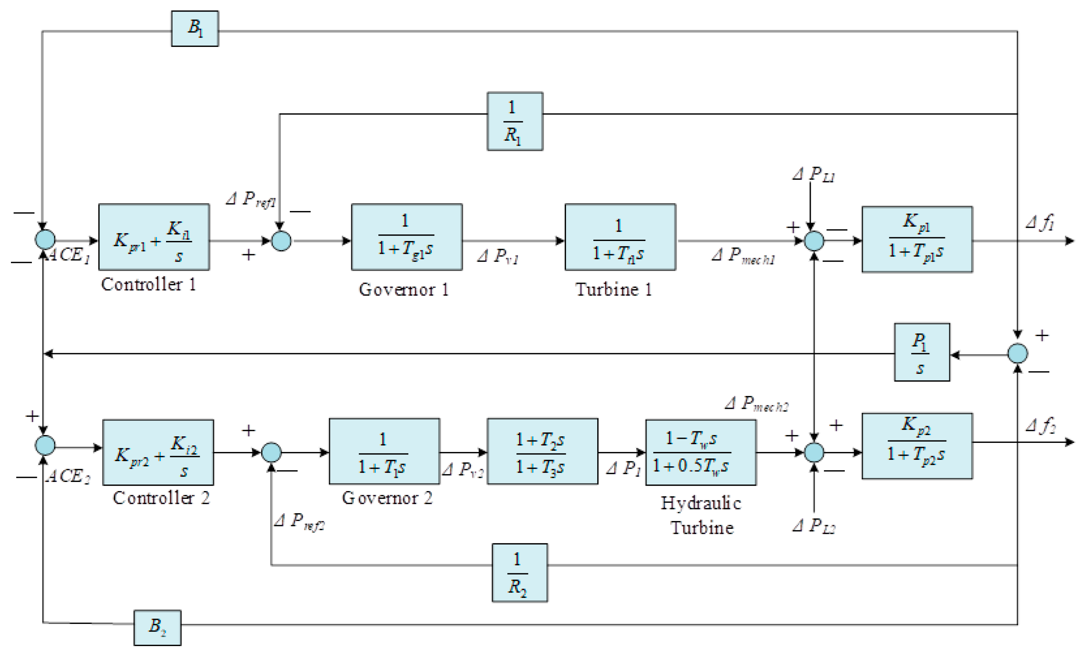
2. State Space Modeling of a Hydrothermal System

This section deals with the PI controller and the modeling of the two-area hydrothermal system using a state space approach.

2.1. The Proportional Plus Integral Controller

We have considered the PI controller for a LFC analysis of the hydrothermal power system. If $e(t)$ represents the error at the input of the PI controller, then its output $u(t)$ can be represented by Equation (1) as given below:

$$u(t)=K_{pr}e(t)+K_i{\displaystyle \int e(t)dt}$$

(1)

where K_pr, and K_i, are the controller parameters. In this paper, we consider the objective function as an integral time absolute error (ITAE) [23]. The ITAE cost function is as given by Equation (2) below.

$$ITAE={\displaystyle \underset{0}{\overset{\infty }{\int }}t\times |e(t)|dt}$$

(2)

2.2. Test Model for the Two-Area Hydrothermal System

In order to obtain a performance analysis of the hydrothermal power system based on hGFA optimization techniques, the test system as illustrated in Figure 1 is considered. The different blocks of the test system are modeled using the standard linearized method and are shown by their respective transfer functions. Here, the two-area power system is considered such that one area consists of a hydropower plant and the other area has a thermal power plant for power generation. Each plant has a PI controller, shown by the transfer function to achieve automatic gain control of the power system.

The model of the test system is obtained using the state space approach detailed in [11]. The state space modeling of the test system and its implementation are discussed in the next subsection.

2.3. State Space Modeling

As shown in Figure 1, the test system comprises two interconnected areas resulting in a hydrothermal power system. Each area consists of one PI controller to achieve AGC based on LF, as well as TLP for effective operation of the power system. With the given model and its transfer functions, the test system can be modeled through multidimensional state space analysis. Using a state space approach corresponding to Equations (3) and (4), the transfer function of the overall hydrothermal power system can be obtained.

$$\dot{x}=Ax+Bu$$

(3)

$$y=Cx+Du$$

(4)

Here, x, y, and u, denotes the state vector, output vector, and input vector, respectively. The different matrices with the real constant model-dependent values of the state space model are represented by variables A, B, C, and D.

On analysis of the state space model, the following equations follow:

$$x={\left[\Delta f_1,\Delta P_{mech1},\Delta P_{v1},\Delta f_2,\Delta P_{mech2},\Delta P_1,\Delta P_{v2},\Delta P_{12},\Delta P_{ref1},\Delta P_{ref2}\right]}^T$$

(5)

$$u={\left[\Delta P_{L1},\Delta P_{L2}\right]}^T$$

(6)

$$y={[\Delta f_1,\Delta f_2,\Delta P_{12}]}^T$$

(7)

These variables are part of the test system’s state space model, which characterizes the entire hydrothermal power system as described in [11]. The state space matrices to construct the transfer function is determined by analyzing the differential equations. These are illustrated below.

$$\stackrel{.}{x_1}=-\frac{1}{T_{p1}}{x}_1+\frac{K_{p1}}{T_{p1}}{x}_2-\frac{K_{p1}}{T_{p1}}{x}_8-\frac{K_{p1}}{T_{p1}}{u}_1$$

(8)

$$\stackrel{.}{x_2}=-\frac{1}{T_{t1}}{x}_2+\frac{1}{T_{t1}}{x}_3$$

(9)

$$\stackrel{.}{x_3}=-\frac{1}{R_1{T}_{g1}}{x}_1-\frac{1}{T_{g1}}{x}_3+\frac{1}{T_{g1}}{x}_9$$

(10)

$$\stackrel{.}{x_4}=-\frac{1}{T_{p2}}{x}_4+\frac{K_{p2}}{T_{p2}}{x}_5+\frac{K_{p2}}{T_{p2}}{x}_8-\frac{K_{p2}}{T_{p2}}{u}_2$$

(11)

$$\stackrel{.}{x_5}=-\frac{2T_2}{R_2{T}_1{T}_3}{x}_4-\frac{2}{T_w}{x}_5+\left(\frac{2}{T_w}+\frac{2}{T_3}\right)x_6+\left(\frac{2T_2}{T_1{T}_3}-\frac{2}{T_3}\right)x_7-\frac{2T_2}{T_1{T}_3}{x}_{10}$$

(12)

$$\stackrel{.}{x_6}=-\frac{T_2}{R_2{T}_1{T}_3}{x}_4-\frac{1}{T_3}{x}_6+\left(\frac{1}{T_3}-\frac{T_2}{T_1{T}_3}\right)x_7+\frac{T_2}{T_1{T}_3}{x}_{10}$$

(13)

$$\stackrel{.}{x_7}=-\frac{1}{R_2{T}_1}{x}_4-\frac{1}{T_1}{x}_7+\frac{1}{T_1}{x}_{10}$$

(14)

$$\stackrel{.}{x_8}=T_s{x}_1-T_s{x}_4$$

(15)

$$\stackrel{.}{x_9}=\left(\frac{B_1{K}_{pr1}}{T_{p1}}-K_{pr1}{T}_s-K_{i1}{B}_1\right)x_1-\frac{B_1{K}_{pr1}{K}_{p1}}{T_{p1}}{x}_2+K_{pr1}{T}_s{x}_4+\left(\frac{B_1{K}_{pr1}{K}_{p1}}{T_{p1}}-K_{i1}\right)x_8+\frac{B_1{K}_{pr1}{K}_{p1}}{T_{p1}}{u}_1$$

(16)

$$\stackrel{.}{x_{10}}=K_{pr2}{T}_s{x}_1+\left(\frac{B_2{K}_{pr2}}{T_{p2}}-K_{pr2}{T}_s-K_{i2}{B}_2\right)x_4-\frac{B_2{K}_{pr2}{K}_{p2}}{T_{p2}}{x}_5+\left(-\frac{B_2{K}_{pr2}{K}_{p2}}{T_{p2}}+K_{i2}\right)x_8+\frac{B_2{K}_{pr2}{K}_{p2}}{T_{p2}}{u}_2$$

(17)

Finally, the state matrices are obtained by incorporating the above differential equations. These are as shown below:

$$A=\left[\begin{array}{cccccccccc}-\frac{1}{T_{P1}}& \frac{K_{P1}}{T_{P1}}& 0& 0& 0& 0& 0& -\frac{K_{P1}}{T_{P1}}& 0& 0\\ 0& -\frac{1}{T_{t1}}& \frac{1}{T_{t1}}& 0& 0& 0& 0& 0& 0& 0\\ -\frac{1}{R_1{T}_{g1}}& 0& \frac{1}{T_{g1}}& 0& 0& 0& 0& 0& \frac{1}{T_{g1}}& 0\\ 0& 0& 0& -\frac{1}{T_{P2}}& \frac{K_{P2}}{T_{P2}}& 0& 0& \frac{K_{P2}}{T_{P2}}& 0& 0\\ 0& 0& 0& \frac{2T_2}{R_2{T}_1{T}_2}& -\frac{2}{T_w}& (\frac{2}{T_w}+\frac{2}{T_3})& (\frac{2T_2}{T_1{T}_3}-\frac{2}{T_3})& 0& 0& -\frac{2T_2}{T_1{T}_3}\\ 0& 0& 0& -\frac{T_2}{R_2{T}_1{T}_2}& 0& -\frac{1}{T_3}& (\frac{1}{T_3}-\frac{T_2}{T_1{T}_3})& 0& 0& \frac{T_2}{T_1{T}_3}\\ 0& 0& 0& -\frac{1}{R_2{T}_1}& 0& 0& -\frac{1}{T_1}& 0& 0& \frac{1}{T_1}\\ T_s& 0& 0& -T& 0& 0& 0& 0& 0& 0\\ A_{9,1}& -\frac{B_1{K}_{pr1}{K}_{P1}}{T_{P1}}& 0& K_{pr1}{T}_s& 0& 0& 0& (\frac{B_1{K}_{pr1}{K}_{P1}}{T_{P1}}-K_{i1})& 0& 0\\ K_{pr2}{T}_s& 0& 0& A_{10,4}& -\frac{B_2{K}_{pr2}{K}_{P2}}{T_{P2}}& 0& 0& (-\frac{B_2{K}_{pr2}{K}_{P2}}{T_{P2}}+K_{i2})& 0& 0\end{array}\right]$$

where,

$$\begin{gathered} A_{9,1}=(\frac{B_1{K}_{pr1}}{T_{P1}}-K_{pr1}{T}_s-K_{i1}{B}_1), A_{10,4}=(\frac{B_2{K}_{pr2}}{T_{P2}}-K_{pr2}{T}_s-K_{i2}{B}_2) \\ B={\left[\begin{array}{cccccccccc}-\frac{K_{P1}}{T_{P1}}& 0& 0& 0& 0& 0& 0& 0& \frac{B_1{K}_{pr1}{K}_{P1}}{T_{P1}}& 0\\ 0& 0& 0& -\frac{K_{P2}}{T_{P2}}& 0& 0& 0& 0& 0& \frac{B_2{K}_{pr2}{K}_{P2}}{T_{P2}}\end{array}\right]}^T \\ C=\left[\begin{array}{cccccccccc}1& 0& 0& 0& 0& 0& 0& 0& 0& 0\\ 0& 0& 0& 1& 0& 0& 0& 0& 0& 0\\ 0& 0& 0& 0& 0& 0& 0& 1& 0& 0\end{array}\right] \\ D=0 \end{gathered}$$

The transfer function (T.F) using matrices A, B, C, and D can be obtained using the relation:

$$T.F=C{\left[SI-A\right]}^{-1}B+D$$

Without loss of generality, the transfer function will be a matrix of the dimension (3 × 2). The elements of the transfer function are as follows.

$$\Delta f_1=\frac{\Delta f_1(s)}{\Delta P_{L1}(s)}\Delta P_{L1}+\frac{\Delta f_1(s)}{\Delta P_{L2}(s)}\Delta P_{L2}$$

(18)

$$\Delta f_2=\frac{\Delta f_2(s)}{\Delta P_{L1}(s)}\Delta P_{L1}+\frac{\Delta f_2(s)}{\Delta P_{L2}(s)}\Delta P_{L2}$$

(19)

$$\Delta P_{12}=\frac{\Delta P_{12}(s)}{\Delta P_{L1}(s)}\Delta P_{L1}+\frac{\Delta P_{12}(s)}{\Delta P_{L2}(s)}\Delta P_{L2}$$

(20)

3. Hybrid Gravitational–Firefly Algorithm

The hybrid gravitational–firefly algorithm uses two well-known optimization techniques, the GSA and the FA [35,36,37,38]. Newton’s gravitational law is the working principle for the GSA. In this, every object is treated as a candidate solution. The masses of each of these variables or the candidate are used to evaluate their performance depending on the value of the selected objective function [21]. On the other hand, the working of the FA is similar to the flashing behavior of fireflies, which they use to achieve communication amongst themselves. The hybrid gravitational–firefly algorithm takes the properties of both these algorithms and updates the values of its objects (candidate solutions) using the updated equations.

3.1. GSA

The position (x) of each agent (i) out of N agents is represented by $x_i$. If we assume $m$ dimensional space, then the position of each agent $x_i^d$ is given using the following equation:

$$x_i=(x_i^1,\dots x_i^d,\dots x_i^m)\forall i=\{1,2,\dots ,N\}$$

(21)

The mass ‘j’ applies force on mass ‘i’, which is given as,

$$F_{ij}^d(t)=G(t)\times \frac{\left(x_j^d(t)-x_i^d(t)\right)}{R_{ij}(t)+\epsilon }\left(M_{pi}(t)\ast M_{aj}(t)\right)$$

(22)

where $G(t)$ denotes the gravitational constant, $R_{ij}(t)$ denotes the Euclidian distance between agent ‘i’ and agent ‘j’, and $M_{pi}(t)$ and $M_{ai}(t)$ represent the passive gravitational and active gravitational masses of the agent ‘i’ and the agent ‘j’, respectively. The Euclidian and the gravitational constants are given as below.

$$\begin{array}{l}{R}_{ij}(t)=\left|\right|x_i(t),x_j(t)|{|}_2\\ G(t)=G(G_0,t)\end{array}\}$$

(23)

If $M_{ii}(t)$ indicates the inertial mass of the ith agent, the total force and the total acceleration acting on an agent ‘i’ due to other agents in the d-dimensional space is given as:

$$F_i^d(t)={\displaystyle \sum _{j=1,j\ne i}^N{rand}_j{F}_{ij}^d(t)}, a_i^d(t)=\frac{F_i^d(t)}{M_{ii}(t)}$$

(24)

In each round, Equations (25) and (26) are used to update the velocity as well as the mass of each agent i.

$$m_i(t)=\frac{{\mathrm{fit}}_i(t)-\mathrm{worst}(t)}{\mathrm{best}(t)-\mathrm{worst}(t)}$$

(25)

$$M_i(t)=\frac{m_i(t)}{{\displaystyle \sum _{j=1}^N{m}_j(t)}}$$

(26)

3.2. Firefly Algorithm

The Euclidian distance between the firefly ‘i’ and firefly ‘j’ for given position x_i and x_j can be evaluated using the equation given below,

$$r_{ij}=\sqrt{{\displaystyle {\sum }_{k=1}^d{(x_{i,k}-x_{j,k})}^2}}$$

(27)

where $k$ indicates the kth element of the spatial coordinates.

The attractiveness parameter of every firefly basically can be given by the following equation:

$$\beta ={\beta }_0{e}^{-\gamma r^2}$$

(28)

where γ represents the coefficient of absorption, which is used to control the light intensity. We can define the movement of each firefly as follows.

$$v_i^d(t+1)={\mathrm{rand}}_i\times v_i^d(t)+a_i^d(t)$$

(29)

$$x_i{}^d=x_i{}^d+{\beta }_0{e}^{-\gamma r_{ij}^2}(x_j-x_i)+v_i^d(t+1)+\alpha \epsilon$$

(30)

Here, x_i is the instantaneous position of an object and $\alpha \epsilon$ indicates the random behavior of a firefly if no brighter firefly is detected.

4. Methodology and Simulation Results

This section presents a methodology to design and configure two-area hydrothermal power systems using simulation to evaluate the performance of the proposed optimization technique.

4.1. Simulation Methodology

To evalute the efficacy of the proposed hybrid gravitational–firefly algorithm, the test system shown in Figure 1 is designed. The test system comprises a two-area power system, one with a thermal power plant and the other with a hydropower plant. To design and configure the two-area power system, MATLAB Simulink is used. Further, the proposed algorithm is coded in a MATLAB script file and then interfaced to the Simulink model for testing its efficacy on the test system.

The various simulation configuration parameters are as follows: MATLAB (R2016a) software is used along with the Simulink tool. The system used for simulation has an i5-6200 CPU@ processor running at 2.30 GHz frequency and having 8 GB RAM. The proposed algorithm and other optimization techniques are written as MATLAB scripts, which are interfaced to the test power system through the Simulink. A few of the other key parameters are included in the Appendix A section.

4.2. Simulation Results

The simulation was performed to evaluate the load frequencies and tie-line parameters of the test system. The simulations were carried out by tuning the parameters of the PI controller using the novel hybrid gravitational search with firefly algorithm as an optimization technique. To understand the efficacy of this algorithm, the results are compared with PSO, GA, GSA, and FA, which can be used as a benchmark for performance evaluation. In all the optimization techniques, the cost function is ITAE and remains unaltered.

The performance of the proposed algorithm on hydrothermal power systems is evaluated by considering two case studies, which are discussed below.

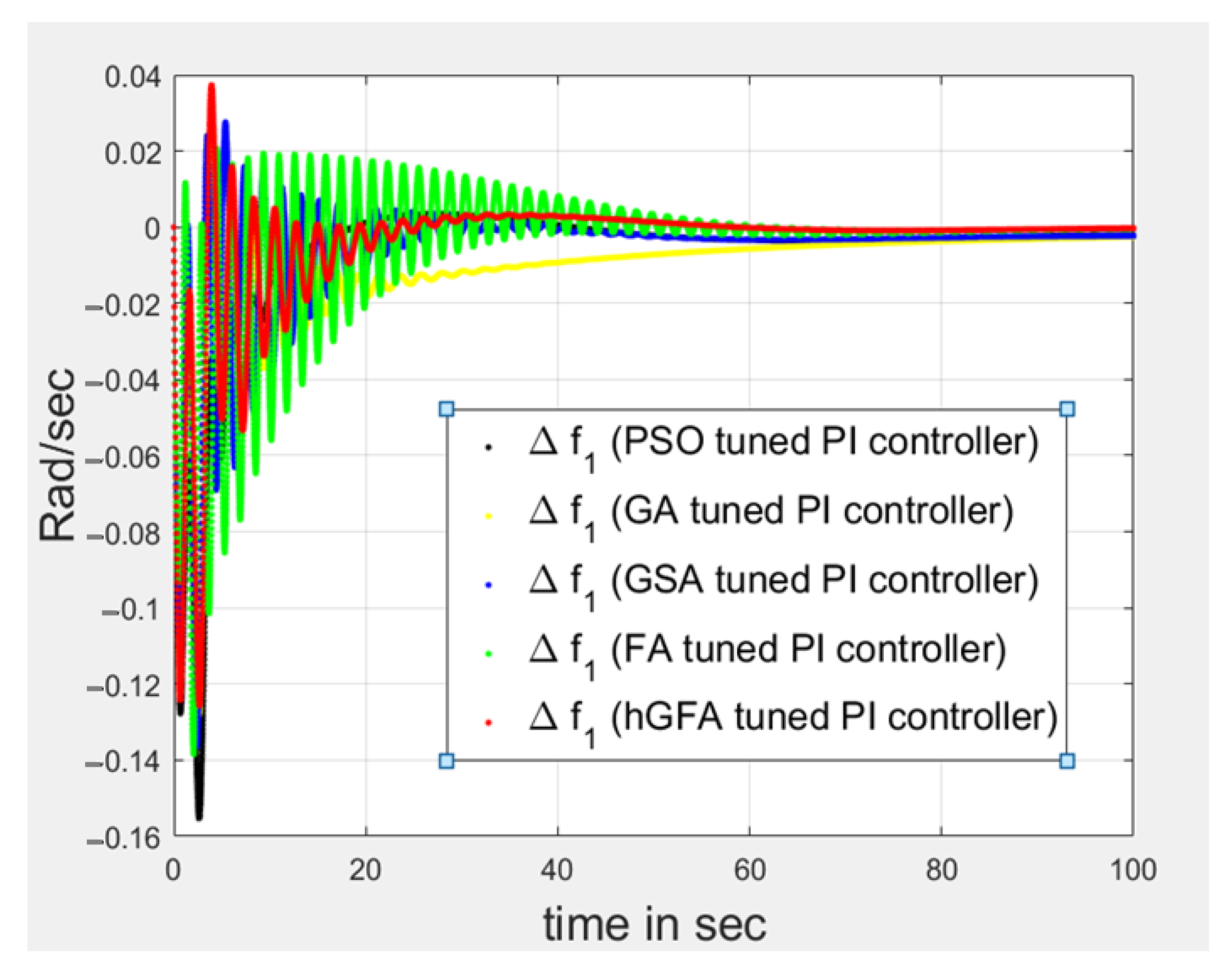
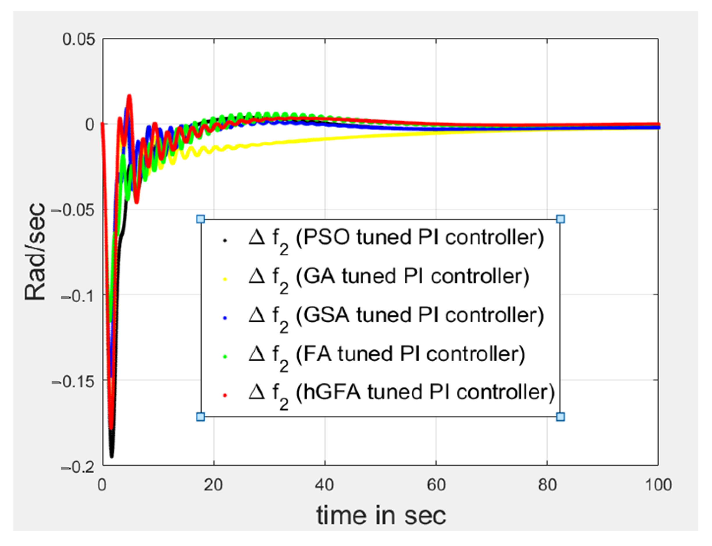
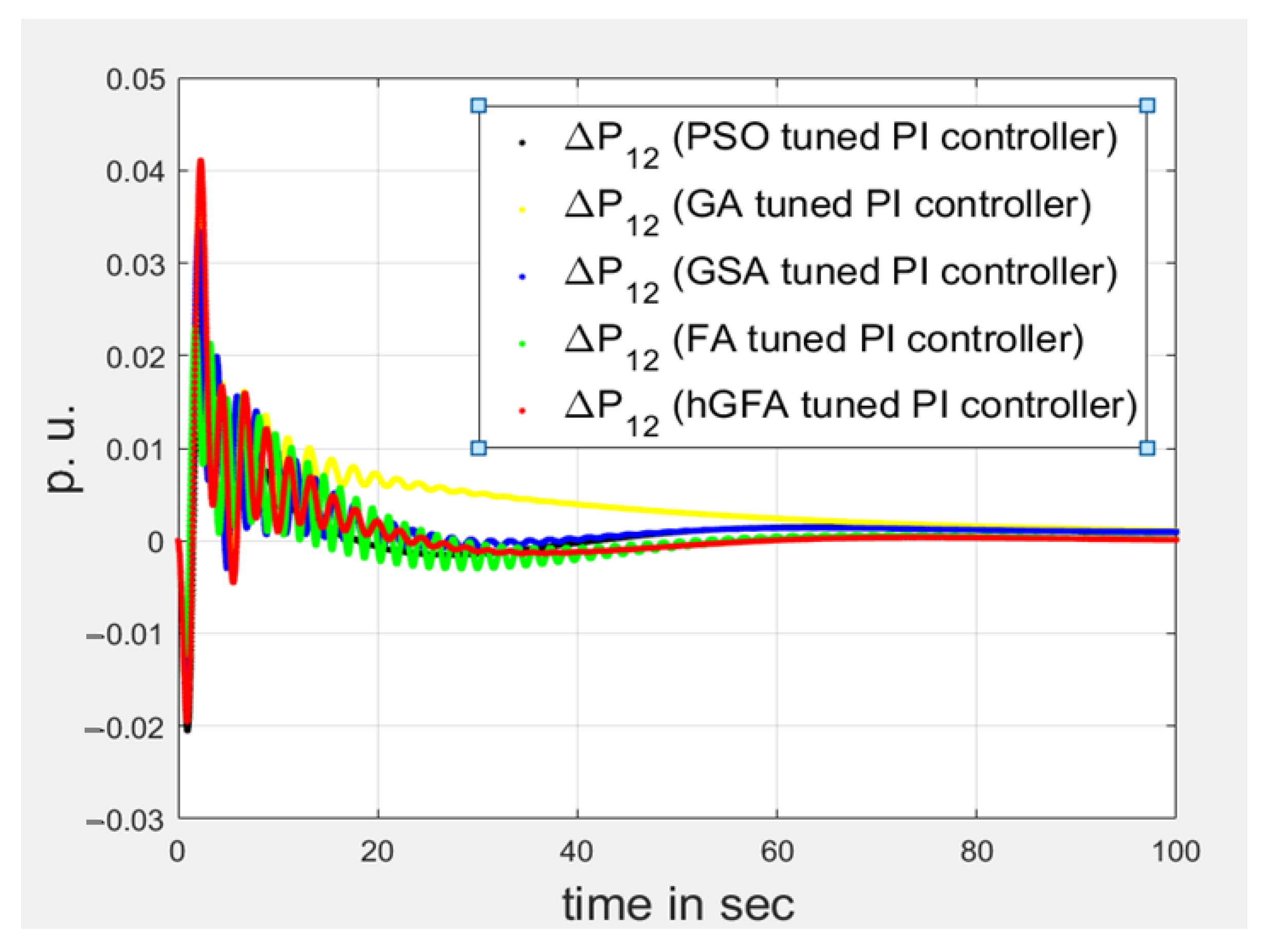
4.2.1. Case Study-I

To observe performance under a step load change, the load in the area having the thermal power plant (area-1) is incremented up to 20%. The load in the area having the hydropower plant (area-2) is unchanged. The test system is simulated using different optimization techniques, i.e., PSO, GA, GSA, FA, and hGFA. ITAE is used as the objective function. The parameters of the PI controller tuned using these optimization techniques are summarized in

Table 1. Optimized parameters of PI controller for case study-I.

O.T.	Kpr1	Kpr2	Ki1	Ki2
GA	0.068627	1.9095	0.33831	0.033451
PSO	0.048043	1.2241	0.75369	0.001
GSA	1.4718	9.1185	0.4606	0.0006
FA	0.6366	5.5908	0.8408	0.0343
hGFA	0.0015	3.3537	0.8210	0.0600

.

The performance of the test system based on LF as well as TLP is analyzed by using the optimized parameters shown in Table 1. The simulation results corresponding to the load frequency in area-1 ($\Delta f_1$), the load frequency in area-2 ($\Delta f_2$), and the tie-line power flow of the test system are shown in Figure 2, Figure 3 and Figure 4, respectively.

4.2.2. Case Study-II

To observe performance under a step load change, the load in the area with a thermal power plant (area-1) is incremented up to 5% and the load in area-2 is subjected to a 1% change. The tuned parameters of the PI controller using different optimization techniques are summarized in

Table 2. Optimized parameters of the PI controller for case study-II.

O.T.	Kpr1	Kpr2	Ki1	Ki2
GA	0.033451	0.092078	0.7018	0.01
PSO	0.0010	1.5064	0.2833	0.0128
GSA	0.4273	1.9126	0.7865	0.0104
FA	1.2880	1.5767	0.5235	0.0333
hGFA	0.0010	1.5534	0.7537	0.0363

.

The simulation results corresponding to the load frequency in area-1 ($\Delta f_1$), the load frequency in area-2 ($\Delta f_2$), and the tie-line power flow of the test system are shown in Figure 5, Figure 6 and Figure 7, respectively.

5. Analysis and Discussion

The simulated results of the test system are analyzed in this section. To perform a comparative analysis, the results achieved using the hGFA are compared with those obtained using the PSO, the GA, the GSA, and the FA. The comparisons are in terms of the overshoot/undershoot, and settling time for the load frequency response and the TLP.

5.1. Case Study-I

For the first case study, for the perturbation in step load change, the load frequency responses in area-1 and area-2 have been shown in Figure 2 and Figure 3, respectively. Figure 4 represents the TLP for the interconnected power system belonging to case study-I. It can be inferred from these responses that the hGFA optimization technique outperforms other optimization techniques. The overshoot/undershoot, and settling time of these results are summarized in

Table 3. Comparison of optimization techniques based on overshoot and settling time for case study-I.

		Case Study
Optimization Techniques	System Variables	Overshoot	Settling Time (s)
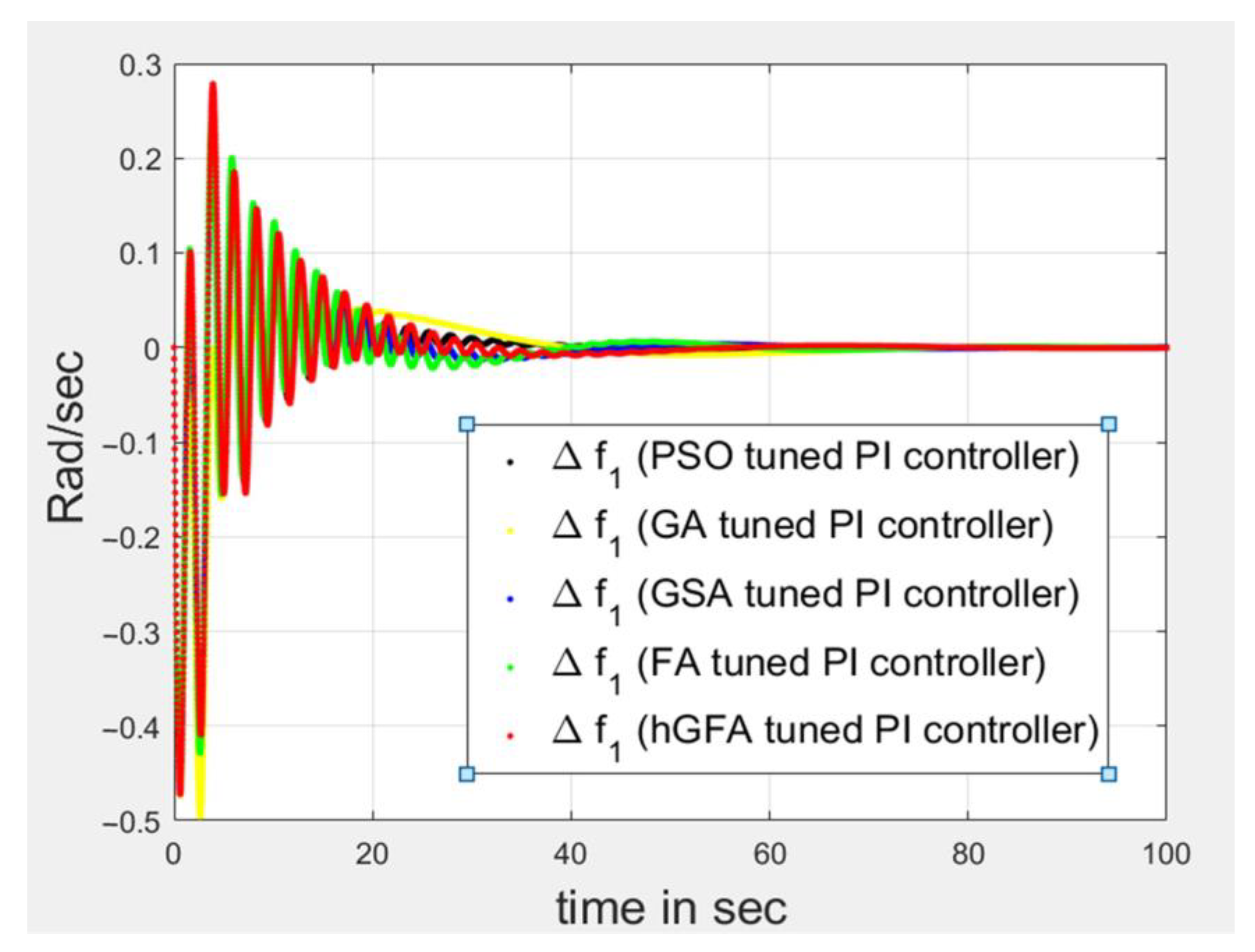
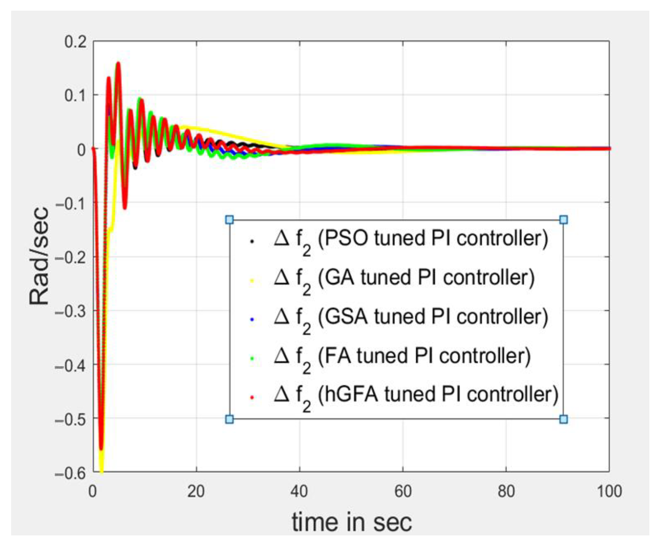
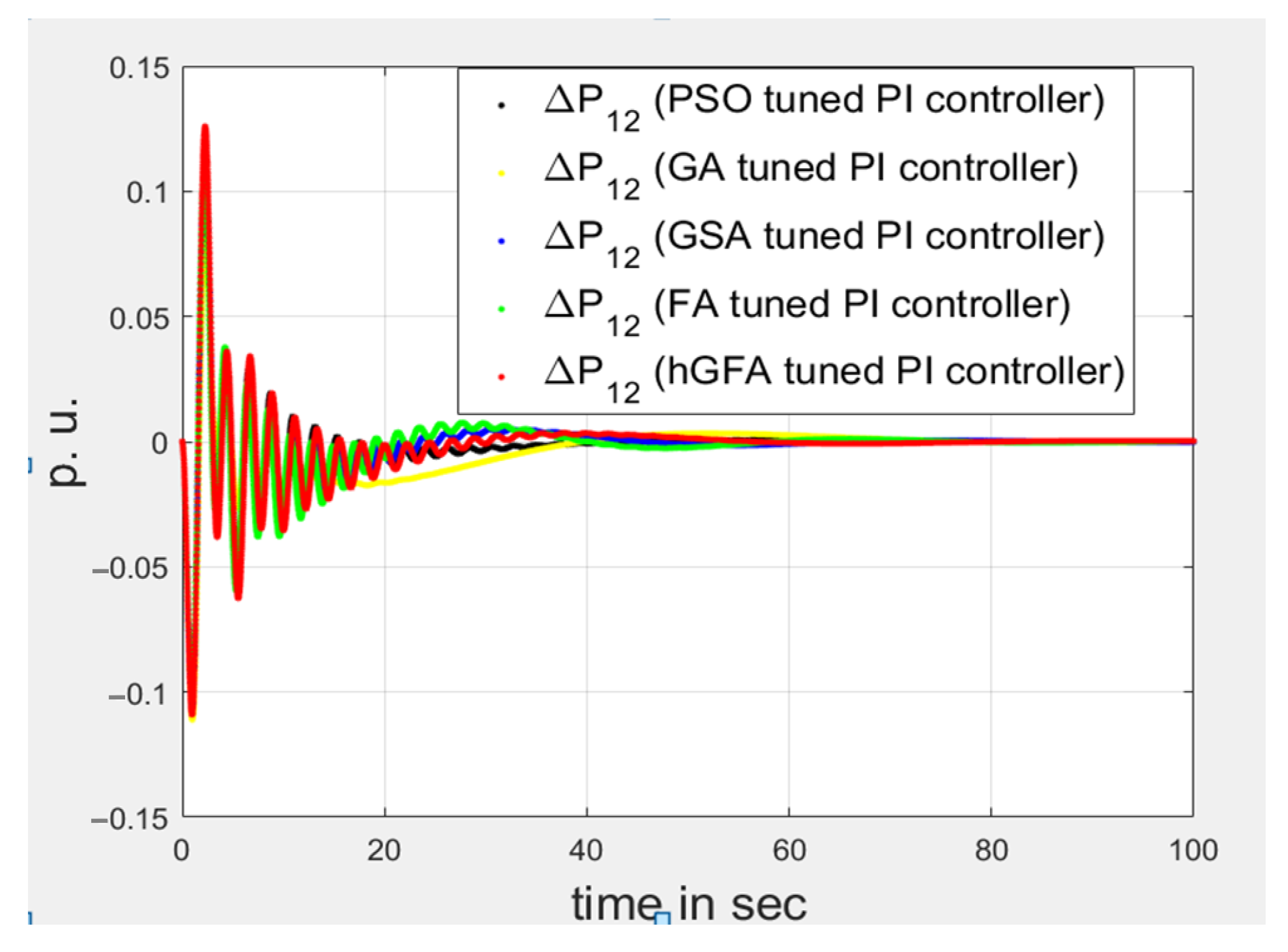
Genetic Algorithm (GA)	∆f1	−0.5	40
	∆f2	−0.6	41
	∆P12	−0.12	45
Particle Swarm Optimization (PSO)	∆f1	−0.47	40
	∆f2	−0.55	38
	∆P12	−0.12	39
Gravitational Search Algorithm (GSA)	∆f1	−0.46	40
	∆f2	−0.52	40
	∆P12	−0.12	43
Firefly Algorithm (FA)	∆f1	−0.47	45
	∆f2	−0.51	43
	∆P12	−0.11	42
Hybrid Gravitational–Firefly Algorithm (hGFA)	∆f1	−0.46	35
	∆f2	−0.50	33
	∆P12	−0.11	35

.

From Table 3, it can be seen that the overshoot/undershoot for the system variable ∆f₁ is −0.46, −0.47, −0.5, −0.46, and −0.47 for the hGFA, the PSO, the GA, the GSA, and the FA, respectively. Further, it can also be seen that the overshoot/undershoot for the system variable ∆f₂ is −0.50, −0.55, −0.6, −0.52, and −0.51, corresponding to the hGFA, the PSO, the GA, the GSA, and the FA, respectively. Furthermore, the system variable ∆P₁₂ is −0.11, −0.12, −0.12, −0.12, and −0.11, corresponding to the hGFA, the PSO, the GA, the GSA, and the FA, respectively. Thus, it can be inferred that the hGFA outperforms other well-known optimization techniques such as PSO, GA, GSA, and FA in terms of overshoot/undershoot for all the system variables of the HTPS. Similarly, it can be inferred by analyzing the results in Table 3 that the hGFA (with T_s = 35 s, 33 s, 35 s, respectively, for ∆f₁, ∆f₂, ∆P₁₂) performs better in terms of settling time (T_s) compared to its competitor optimization techniques such as PSO (with T_s = 40 s, 38 s, 39 s, respectively, for ∆f₁, ∆f₂, ∆P₁₂), GA (with T_s = 40 s, 41 s, 45 s, respectively, for ∆f₁, ∆f₂, ∆P₁₂), GSA (with T_s = 40 s, 40 s, 43 s, respectively, for ∆f₁, ∆f₂, ∆P₁₂), and FA (with T_s = 45 s, 43 s, 42 s, respectively, for ∆f₁, ∆f₂, ∆P₁₂). Hence, it can be concluded that, for case study-I, the performance of the proposed hybrid optimization technique is better than other optimization techniques.

5.2. Case Study-II

From the perturbation in responses of frequencies in both the area as well as tie-line power, illustrated in Figure 5, Figure 6 and Figure 7, it can be inferred that the hGFA optimization technique performs better compared to other techniques. The overshoot/undershoot and settling time for different system variables are summarized in

Table 4. Comparison of optimization techniques based on overshoot/undershoot and settling time for case study-II.

		Case Study
Optimization Techniques	System Variables	Overshoot	Settling Time (s)
Genetic Algorithm (GA)	∆f1	−0.13	75
	∆f2	−0.17	70
	∆P12	−0.02	70
Particle Swarm Optimization (PSO)	∆f1	−0.158	70
	∆f2	−0.2	60
	∆P12	−0.021	45
Gravitational Search Algorithm (GSA)	∆f1	−0.15	65
	∆f2	−0.15	65
	∆P12	−0.018	70
Firefly Algorithm (FA)	∆f1	−0.14	70
	∆f2	−0.12	60
	∆P12	−0.014	70
Hybrid Gravitational–Firefly Algorithm (hGFA)	∆f1	−0.12	35
	∆f2	−0.17	30
	∆P12	−0.02	30

.

From Table 4, it can be seen that the overshoot/undershoot for the system variable ∆f₁ is −0.12, −0.158, −0.13, −0.15, and −0.14, corresponding to hGFA, PSO, GA, GSA, and FA, respectively. Further, it can also be seen that the overshoot/undershoot for the system variable ∆f₂ is −0.17, −0.2, −0.17, −0.15, and −0.12, corresponding to hGFA, PSO, GA, GSA, and FA, respectively. The system variable ∆P₁₂ is −0.02, −0.021, −0.02, −0.018, and −0.014, corresponding to hGFA, PSO, GA, GSA, and FA, respectively. Similarly, by analyzing Table 4, it can be seen that the hGFA (with T_s = 35 s, 30 s, 30 s, respectively, for ∆f₁, ∆f₂, ∆P₁₂) performs better in terms of settling time (T_s) compared to its competitor optimization techniques such as PSO (with T_s = 70 s, 60 s, 45 s, respectively, for ∆f₁, ∆f₂, ∆P₁₂), GA (with T_s = 75 s, 70 s, 70 s, respectively, for ∆f₁, ∆f₂, ∆P₁₂), GSA (with T_s = 65 s, 65 s, 70 s, respectively, for ∆f₁, ∆f₂, ∆P₁₂), and FA (with T_s = 70 s, 60 s, 70 s, respectively, for ∆f₁, ∆f₂, ∆P₁₂). These algorithms offer similar overshoot/undershoot characteristics, but the settling time characteristics vary. The proposed algorithm reduces the settling time considerably, by approximately 50% when compared to other techniques.

6. Conclusions

The TAS consideration of hydrothermal systems is considered in this paper for LFC as well as TLP analysis. Each area has been considered with a proportional integral controller for analysis. The parameters of each PI controller are tuned using several optimization techniques with ITAE as an objective function. From the in-depth simulation presented in Section 4, followed by the analysis in Section 5, it has been observed that the proposed hGFA performs better than the other optimization techniques. Further, the hGFA improves the response of the interconnected power system, resulting in low overshoot and reduced settling time for LF as well as TLP flow. The main findings of this study can be summarized as follows:

• The novel optimization technique, hGFA, based on the GSA and the FA, is proposed in this paper to address the LFC and tie-line power flow issues of the two-area HTPS.
• The performance of the proposed algorithm is compared with other well-known optimization techniques such as PSO, GA, GSA, and FA using ITAE as the objective function.
• For almost the same overshoot, the settling time value of the LF as well as the TLP is lowered by almost 15% in case study-I, and it is lowered by almost 50% in case study-II using the proposed hGFA, as compared to PSO, GA, GSA, and FA.
• The computation time is almost the same for all algorithms analyzed in this study, so the complexity of the proposed algorithm remains comparable to the basic algorithms and is used as a benchmark for evaluating performance.

Hence, it can be inferred that the hGFA outperforms the other optimization techniques (PSO, GA, GSA, and FA). Therefore, it can be successfully applied for AGC of a hydrothermal power system.

References

- Tabatabaei, N.M.; Kabalci, E.; Bizon, N. Microgrid Architectures, Control and Protection Methods, 1st ed.; Springer: London, UK, 2019. [Google Scholar]
- Thounthong, P.; Mungporn, P.; Pierfederici, S.; Guilbert, D.; Bizon, N. Adaptive Control of Fuel Cell Converter Based on a New Hamiltonian Energy Function for Stabilizing the DC Bus in DC Microgrid Applications. Mathematics 2020, 8, 2035. [Google Scholar] [CrossRef]
- Tabatabaei, N.M.; Ravadanegh, S.N.; Bizon, N. Power Systems Resiliency: Modeling, Analysis and Practice; Springer: London, UK, 2018. [Google Scholar]
- Li, Y.; Zhang, H.; Liang, X.; Huang, B. Event-Triggered-Based Distributed Cooperative Energy Management for Multienergy Systems. IEEE Trans. Industr. Inform. 2019, 15, 2008–2022. [Google Scholar] [CrossRef]
- Yushuai, L.; Gao, W.; Gao, W.; Zhang, H.; Zhou, J. A Distributed Double-Newton Descent Algorithm for Cooperative Energy Management of Multiple Energy Bodies in Energy Internet. IEEE Trans. Industr. Inform. 2020. [Google Scholar] [CrossRef]
- Zhou, J.; Xu, Y.; Sun, H.; Li, Y.; Chow, M. Distributed Power Management for Networked AC–DC Microgrids with Unbalanced Microgrids. IEEE Trans. Industr. Inform. 2020, 16, 1655–1667. [Google Scholar] [CrossRef]
- Jha, A.V.; Ghazali, A.N.; Appasani, B.; Ravariu, C.; Srinivasulu, A. Reliability Analysis of Smart Grid Networks Iincorporating Hardware Failures and Packet Loss. Rev. Roum. Sci. Tech. El. 2021, 65, 245–252. [Google Scholar]
- Mishra, S.K.; Bhargav, A.; Jha, A.V.; Garrido, I.; Garrido, A.J. Centralized Airflow Control to Reduce Output Power Variation in a Complex OWC Ocean Energy Network. Complexity 2020, 2020, 2625301. [Google Scholar] [CrossRef]
- Jha, A.V.; Ghazali, A.N.; Appasani, B.; Mohanta, D.K. Risk Identification and Risk Assessment of Communication Networks in Smart Grid Cyber-Physical Systems. In Security in Cyber-Physical Systems; Studies in Systems, Decision and Control; Awad, A.I., Furnell, S., Paprzycki, M., Sharma, S.K., Eds.; Springer: Cham, Switzerland, 2021; Volume 339. [Google Scholar] [CrossRef]
- Li, Y.; Gao, W.; Yan, W.; Huang, S.; Wang, R.; Gevorgian, V.; Gao, D.W. Data-Driven Optimal Control Strategy for Virtual Synchronous Generator via Deep Reinforcement Learning Approach. J. Mod. Power Syst. Clean Energy 2021, 9, 27–36. [Google Scholar] [CrossRef]
- Saadat, H. Power System Analysis, 2nd ed.; McGraw-Hill: New York, NY, USA, 2009. [Google Scholar]
- Kundur, P. Power System Stability and Control, 1st ed.; McGraw-Hill: New York, NY, USA, 1994. [Google Scholar]
- Wood, A.J.; Woolenberg, B.F. Power Generation Operation and Control, 3rd ed.; John Wiley and Sons: Hoboken, NJ, USA, 1984. [Google Scholar]
- Nanda, J.; Kaul, B.L. Automatic generation control of an interconnected power system. Proc. IEEE 1978, 125, 385–390. [Google Scholar] [CrossRef]
- Working Group Prime Mover and Energy Supply. Hydraulic turbine and turbine control models for system dynamic studies. IEEE Trans. Power Syst. 1992, 7, 167–179. [Google Scholar] [CrossRef]
- Khodabakhshian, A.; Golbon, N. Unified PID design for load frequency control. In Proceedings of the International Conference on Control Applications, Taipei, Taiwan, 2–4 September 2004; IEEE: New York, NY, USA, 2004; pp. 1627–1632. [Google Scholar] [CrossRef]
- Nanda, J.; Kothari, M.L.; Satsangi, P.S. Automatic generation control of an interconnected hydrothermal system in continuous and discrete modes considering generation rate constraints. Proc. Inst. Elect. Eng. 1983, 130, 17–27. [Google Scholar] [CrossRef]
- Ramakrishna, K.S.S.; Bhatti, T.S. Load Frequency Control of Interconnected Hydro-Thermal Power Systems. In Proceedings of the International Conference on Energy and Environment, New Delhi, India, Month–August 2006; Available online: https://scholar.google.com/scholar?hl=en&as_sdt=0%2C5&q=Load+frequency+control+of+interconnected+hydro-thermal+power+systems&btnG= (accessed on 7 February 2021).
- Jha, A.V.; Gupta, D.K.; Appasani, B. The PI Controllers and its optimal tuning for Load Frequency Control (LFC) of Hybrid Hydro-thermal Power Systems. In Proceedings of the International Conference on Communication and Electronics Systems (ICCES), Coimbatore, India, 17–19 July 2019; IEEE: New York, NY, USA, 2019; pp. 1866–1870. [Google Scholar] [CrossRef]
- Arora, K.; Kumar, A.; Kamboj, V.K.; Prashar, D.; Shrestha, B.; Joshi, G.P. Impact of Renewable Energy Sources into Multi Area Multi-Source Load Frequency Control of Interrelated Power System. Mathematics 2021, 9, 186. [Google Scholar] [CrossRef]
- Gupta, D.K.; Naresh, R.; Jha, A.V. Automatic Generation Control for Hybrid Hydro-Thermal System using Soft Computing Techniques. In 2018 5th IEEE Uttar Pradesh Section International Conference on Electrical, Electronics and Computer Engineering (UPCON 2018), Proceedings of the 5th IEEE Uttar Pradesh Section International Conference on Electrical, Electronics and Computer Engineering (UPCON), Gorakhpur, India, 2–4 September 2018; IEEE: New York, NY, USA, 2018; pp. 1–6. [Google Scholar] [CrossRef]
- Prakash, S.; Sinha, S.K. Application of artificial intelligent and load frequency control of interconnected power system. Int. J. Eng. Sci. Technol. 2011, 3, 377–384. [Google Scholar] [CrossRef]
- Gupta, D.K.; Jha, A.V.; Appasani, B.; Srinivasulu, A.; Bizon, N.; Thounthong, P. Load Frequency Control Using Hybrid Intelligent Optimization Technique for Multi-Source Power Systems. Energies 2021, 14, 1581. [Google Scholar] [CrossRef]
- Koley, I.; Bhowmik, P.S.; Datta, A. Load frequency control in a hybrid thermal-wind-photovoltaic power generation system. In Proceedings of the 4th International Conference on Power, Control & Embedded Systems (ICPCES), Allahabad, India, 9–11 March 2017; IEEE: New York, NY, USA, 2017; pp. 1–5. [Google Scholar] [CrossRef]
- Khadanga, R.K.; Kumar, A. Hybrid adaptive ‘gbest’-guided gravitational search and pattern search algorithm for automatic generation control of multi-area power system. IET Gener. Transm. Distrib. 2016, 11, 3257–3267. [Google Scholar] [CrossRef]
- Khezri, R.; Oshnoei, A.; Oshnoei, S.; Bevrani, H.; Muyeen, S.M. An intelligent coordinator design for GCSC and AGC in a two-area hybrid power system. Appl. Soft Comput. 2019, 76, 491–504. [Google Scholar] [CrossRef]
- Gondaliya, S.; Arora, K. Automatic generation control of multi area power plants with the help of advanced controller. Int. J. Eng. Res. Technol. 2015, 4, 470–474. [Google Scholar] [CrossRef]
- Gheisarnejad, M.; Khooban, M.H. Secondary load frequency control for multi-microgrids: HiL real-time simulation. Soft Comput. 2019, 23, 5785–5798. [Google Scholar] [CrossRef]
- Çelik, E. Design of new fractional order PI–fractional order PD cascade controller through dragonfly search algorithm for advanced load frequency control of power systems. Soft Comput. 2020, 25, 1–25. [Google Scholar] [CrossRef]
- Ionescu, L.-M.; Bizon, N.; Mazare, A.-G.; Belu, N. Reducing the Cost of Electricity by Optimizing Real-Time Consumer Planning Using a New Genetic Algorithm-Based Strategy. Mathematics 2020, 8, 1144. [Google Scholar] [CrossRef]
- Haes Alhelou, H.; Hamedani Golshan, M.E.; Hajiakbari Fini, M. Wind driven optimization algorithm application to load frequency control in interconnected power systems considering GRC and GDB nonlinearities. Electr. Power Compon. Syst. 2018, 46, 1223–1238. [Google Scholar] [CrossRef]
- Attia, A.E.-F.; Mohammed, A.E.-H. Efficient frequency controllers for autonomous two-area hybrid microgrid system using social-spider optimizer. IET Gener. Transm. Distrib. 2017, 11, 637–648. [Google Scholar]
- Nikmanesh, E.; Hariri, O.; Shams, H.; Fasihozaman, M. Pareto design of Load Frequency Control for interconnected power systems based on multi-objective uniform diversity genetic algorithm (MUGA). Int. J. Electr. Power Energy Syst. 2016, 80, 333–346. [Google Scholar] [CrossRef]
- Sahu, P.C.; Mishra, S.; Prusty, R.C.; Panda, S. Improved-salp swarm optimized type-II fuzzy controller in load frequency control of multi area islanded AC microgrid. Sustain. Energy Grids Netw. 2018, 16, 380–392. [Google Scholar] [CrossRef]
- Yang, X.S. Nature-Inspired Metaheuristic Algorithms, 2nd ed.; Luniver Press: Beckington, UK, 2008. [Google Scholar]
- Rashedi, E.; Nezamabadi-Pour, H.; Saryazdi, S. GSA: A gravitational search algorithm. Inf. Sci. 2009, 179, 2232–2248. [Google Scholar] [CrossRef]
- Kennedy, J.; Eberhart, R. Particle swarm optimization. In Proceedings of the 1995 IEEE International Conference on Neural Networks, Perth, WA, Australia, 27 November–1 December 1995; IEEE: New York, NY, USA; Volume 4, pp. 1942–1948. [Google Scholar] [CrossRef]
- Zhu, H.; Wang, Y.; Ma, Z.; Li, X. A Comparative Study of Swarm Intelligence Algorithms for UCAV Path-Planning Problems. Mathematics 2021, 9, 171. [Google Scholar] [CrossRef]