Article

A Simple and Safe Strategy for Improving the Fuel Economy of a Fuel Cell Vehicle

by
Nicu Bizon
1,2,3,* and
Phatiphat Thounthong
4,5
1
Faculty of Electronics, Communication and Computers, University of Pitesti, 1 Targul din Vale, 110040 Pitesti, Romania
2
ICSI Energy Department, National Research and Development Institute for Cryogenic and Isotopic Technologies, 1 Uzinei, 240050 Ramnicu Valcea, Romania
3
Doctoral School, Polytechnic University of Bucharest, 313 Splaiul Independentei, 060042 Bucharest, Romania
4
Renewable Energy Research Centre (RERC), Department of Teacher Training in Electrical Engineering, Faculty of Technical Education, King Mongkut’s University of Technology North Bangkok, 1518 Pracharat 1 Road, Wongsawang, Bangsue, Bangkok 10800, Thailand
5
Group of Research in Electrical Engineering of Nancy (GREEN), University of Lorraine, 2 Avenue de la Forêt de Haye, 54518 Vandeuvre lès Nancy CEDEX, F-54000 Nancy, France
*
Author to whom correspondence should be addressed.
Mathematics 2021, 9(6), 604; https://doi.org/10.3390/math9060604
Submission received: 10 February 2021 / Revised: 4 March 2021 / Accepted: 5 March 2021 / Published: 11 March 2021

Abstract

:
A new real-time strategy is proposed in this article to optimize the hydrogen utilization of a fuel cell vehicle, by switching the control references of fueling regulators, based on load-following. The advantages of this strategy are discussed and compared, with advanced strategies that also use the aforementioned load-following mode regulator of fueling controllers, but in the entire loading range, respectively, with a benchmark strategy utilizing the static feed-forward control of fueling controllers. Additionally, the advantages of energy-storage function in a charge-sustained mode, such as a longer service life and reduced size due to the implementation of the proposed switching strategy, are presented for the dynamic profiles across the entire load range. The optimization function was designed to improve the fuel economy by adding to the total power of the fuel utilization efficiency (in a weighted way). The proposed optimization loop will seek the reference value to control the fueling regulator in real-time, which is not regulated by a load-following approach. The best switching threshold between the high and low loading scales were obtained using a sensitivity analysis carried out for both fixed and dynamic loads. The results obtained were promising—(1) the fuel economy was two-times higher than the advanced strategies mentioned above; and (2) the total fuel consumption was 13% lower than the static feed-forward strategy. This study opens new research directions for fuel cell vehicles, such as for obtaining the best fuel economy or estimating fuel consumption up to the first refueling station on the planned road.

1. Introduction

In the coming decades, energy and environmental issues will become the most important challenges for researchers working in the sustainable development of energy sector [1,2]. The proton exchange membrane fuel cell (PEMFC) system is usually utilized as green secondary energy generator for hybrid power systems (HPS), based on renewable energy for balancing power flow stability on the DC grid, due to the variability of energy flows from the load and from renewable sources [3,4]. Thanks to its advantages as compared to other fuel cell (FC) technologies, such as very low pollutant emissions, high specific energy, low operating temperature, and a fast start, the PEMFC system is now the most widely used FC type in portable [5,6] and space applications [7,8].
The design of effective control approaches [8,9] and optimization methods [10,11] needs accurate PEMFC dynamic models [12,13]. It was demonstrated that high ripples on FC power (especially in the low frequency band up to hundreds of Hz) or load pulses [14], produce mechanical stress on the proton exchange membrane (PEM), and as a consequence, cause a rapid degradation of the FC lifetime [15,16]. The main stresses were analyzed in [15], highlighting how the mechanical damage of the PEM membrane was effectively produced. The causes and consequences of gas starvation, together with potential mitigation methods, are presented in [16]. The issue of cold start under subfreezing temperatures is experimentally analyzed in [17]. The consequences of frequent start–stop operations are addressed in [18]. Additionally, some recommendations to boost the FC durability and lifetime are given in [16,17]. Thus, fault-tolerant strategies and advanced control methods are proposed to operate the PEMFC power source in safe conditions [19,20].
This paper proposes a load-following (LFW) switching management of fueling flow rates that might optimally operate the PEMFC system. The safety measures for smooth switching of the fueling controllers were considered as well.
The load-following management was studied to handle the load dynamics [21,22] and then extended to an unknown load profile [23]. Impacts of load profiles on the PEMFC system efficiency, but also on safe functioning of the PEMFC power source, are analyzed in [24,25].
The energy supplied by the FC power source can be controlled by using the air regulator [26,27,28,29,30,31,32,33,34,35,36] or the fuel regulator [37,38,39,40], or by switching the fueling regulators, utilizing the strategy proposed in this study.
The air regulator is set to ensure the needed oxygen parameters for the FC stack cathode (the flow and pressure depending on the system load demand) [26]. The air compressor delivers the needed air (with about 21% oxygen) for the electrochemical reaction, ensuring an oxygen excess ratio higher than 1, to avoid the oxygen starvation phenomenon (which might appear during the load pulses) [6,27,28]. The oxygen excess ratio is controlled using different techniques, as follows—(1) feed-forward control [26,29]; (2) PID-based control [30] and its variants (such as optimal PID plus fuzzy controller [31]), feed-forward PID controller [32], and robust PI control [33]; (3) control techniques based on artificial intelligence concepts like fuzzy logic [34,35], neural networks [36], and genetic operators [37]; (4) model predictive control (MPC) based on constrained model [38], linearization method of the model [39,40], and multivariable nonlinear MPC [41,42]; (5) sliding control using the adaptive sliding mode (Lyapunov-based) [43], high-order sliding mode [44,45], sliding mode (nonlinear multivariable) [46], cascade adaptive sliding mode [47], or a combination of sliding mode with flatness control [48] and super-twisting algorithms [49,50]; (6) robust control based on reduced order model [51] or a load governor [52]; and (7) model reference adaptive control (MRAC) [53].
The MRAC technique [53] can prevent compressor surge better than the MPC techniques mentioned above [38,39,40,41,42]. The robustness analysis performed in [33,51,52] for robust control techniques highlights the advantages of using robust control as compared to classic control techniques, such as feed-forward control [26,29] or PID-based control [30,31,32] techniques. However, the feed-forward control [26] is simple, involves low computation, as compared to control techniques based on artificial intelligence concepts [34,35,36,37], and is already implemented in commercial solutions. Consequently, the feed-forward regulator is utilized as a reference in this study.
Nonlinear control techniques based on different sliding modes that combine the nonlinear terms of the super-twisting approach have the advantage of high robustness and good response to disturbances (achieving a short convergence time) [49,50]. For example, the nonlinear multivariable sliding mode control proposed in [46] reduces the dynamics of oxygen excess percentage and also the power fed by the air compressor.
It is known that the power fed by the air compressor is equal to 15% of the FC power. Therefore, new air compressors must be developed, with lower energy consumption and better dynamics [54]. The dynamics of the air compressor makes the air-feed subsystem slower, as compared to the hydrogen subsystem [55,56]. Thus, the authors of this paper focused on oxygen excess percentage control techniques to improve the response of the air-feed subnetwork. This study uses the nonlinear dynamic model proposed in [57] for the air compressor.
The fuel-feed and air-feed subsystems give great importance to safety, when generating the FC power requested by the dynamic load [9,29,58,59], in order to avoid fuel starvation [60]. The following techniques are proposed to control the fuel-feed subsystem—multi-input-multi-output (MIMO) nonlinear control [60], linear quadratic Gaussian (LQG) control [61], nonlinear control [62,63], linear and nonlinear control [64,65], nonlinear MPC [66,67], and sliding mode control [67,68]. An important task is to maintain the stoichiometric ratio for gases under variable load demand profiles [69], due to nitrogen addition [70] and fuel recirculation, using both ejector and blower [65,71]. Thus, in order to optimize the anodic purge techniques, different control methods were proposed to find the optimal purge interval [72], based on a state observer [73], adaptive strategies [74,75], bleeding strategies [75,76], and intelligent control [77]. The anode bleeding strategies manage the nitrogen diffusion through a continuous and controlled leak of gases, by combining the discontinuous classic purge mode with nonlinear control of the fuel-feed subsystem [78,79].
Degradation analysis of the PEMFC system in dead-end operating modes were analyzed in [80,81] and [82] as an effect of variable thermal and pressure conditions, and low-quality hydrogen, respectively. The methods to increase the lifetime of the FC system and avoid potential carbon monoxide poisoning are also presented. To progress the lifetime of the FC generator [29,56,59], the research was focused on thermal [83,84] and water [85,86] subsystems, but also on other FC subsystems, because these are all interconnected and interdependent [87]. Therefore, a systemic methodology based on an integrated approach is recommended to optimize the FC system [88,89]. Thus, new optimization strategies were studied for the FC system [90], FC cars [28,91], and FC hybrid power sources [92], based on nonlinear control [93], state diagram [94,95], MPC [96,97], droop control [98], fuzzy control [99,100], data fusion approach [101], global optimization using the extremum seeking (GES) approach [102], dynamic programming method [103], or Pontryagin’s minimum algorithm [104]. Except for the global optimization strategies, the other strategies mentioned above showed a less than 100% strike ratio in searching for the optimal level of the considered optimization function or could not find it [102]. The optimization function might be designed for different objectives, such as fuel economy [105,106], lifetime extension for FC system [107], or battery stack [99,108], and safe operation of all subsystems [109].
Thus, the real-time strategy analyzed here (and mentioned below as the SW–LFW strategy) minimizes the hydrogen consumption, using a new load-following switching control for the oxygen and hydrogen controllers of the FC generator, which in comparison with the real-time strategy proposed in [110] is simpler (because it uses only one optimization loop instead of two), safer (because the second optimization loop is not involved in setting the set-points of the fueling controllers, and thus some perturbation (pulses) in the desired points of the fueling regulators due to the switching control are avoided), and almost the same fuel economy is obtained. Therefore, the same load profiles used in [110] are also used here to evaluate the results obtained.
Another aim of this work was to compare the performance of the SW–LFW strategy with other strategies, such as the Air–LFW technique [111] and the Fuel–LFW approach [112], which use the load-following set for the hydrogen regulator or oxygen regulator, respectively, in the entire loading scale. The main benefit of the load-following regulator (employed for one of the fueling regulators [111,112] or for both regulators [110]) is the battery operation in a charge-sustained approach [113], which substantially improved the battery’s lifespan [114]. The FC power source generates the required power on the DC grid, according to the load demand. Thus, the hybrid ultracapacitor/battery energy storage system (ESS) only compensate minor differences between the load demand and the FC power. Therefore, the size of the battery might be reduced, as compared to rule-based techniques (where the battery is charged and discharged to sustain the power flow stability on the DC grid due to load dynamics and renewable energy variability, if the renewable energy is available to sustain a part of the load demand [115]).
Therefore, as the results obtained show, the advantages of the load-following control proposed in this paper are the following—(1) increases the battery lifetime; (2) reduces the battery size; and (3) removes need for monitoring the state-of-charge (SOC).
For a fair comparison of the techniques analyzed here, the same optimization function and test conditions are used, and a sensitivity analysis is functioned to obtain the best threshold between the high and low loading ranges (in a manner similar to [116], to obtain the best weighting parameters of the optimization function).
The optimization function is designed (using appropriate weighting parameters [116]) to minimize the hydrogen consumption by adding fuel efficiency to the FC net power (which is usually used as the optimization function of the FC energy efficiency [34,35,36]). The optimization loop solves the optimum value of the FC current, in real-time, which is used to regulate the fuel controller and the air regulator under the Air–LFW and Fuel–LFW approaches, respectively. In case of the SW–LFW strategy, the fueling regulator, which is not controlled on the basis of the load-following technique is used to improve the fuel economy, using this real-time optimization loop.
The results obtained in the case of a variable load underline a hydrogen economy for the proposed strategy, which is double in comparison to the basic strategies mentioned above (about 2.23-times and 2.47-times higher for the Air–LFW and Fuel–LFW techniques, respectively).
The hydrogen economy using the proposed strategy was compared to that of the benchmark strategy using the static feed-forward (sFF) control for the fueling regulators [59]. It is worth mentioning that the reduction of the total fuel consumption was more than 13% using the SW–LFW method, as compared to the sFF approach in the case of a variable outline of the system load demand.
Additionally, the better fuel saving method that uses the SW–LFW technique, as compared to basic strategies of the Air–LFW and Fuel–LFW, was obtained by choosing the best strategy from these two for a certain load level. It was proven that the optimum fuel saving was obtained using the Air–LFW for high-load levels and the Fuel–LFW strategy for low-load levels. Therefore, the best load threshold (between the high and low loading ranges) would be obtained on the basis of the sensitivity analysis functioned for both constant and variable loads.
Therefore, the key findings and novelty of this work are as follows—(1) a scheme for a new optimization approach (the SW–LFW strategy) for better fuel economy of the FC system; (2) the fuel efficiency was compared using the SW–LFW strategy, and the advanced Air–LFW and Fuel–LFW strategies; (3) the fuel economy obtained with the SW–LFW strategy and the sFF control-based strategy was also compared; (4) the advantages related to battery lifetime and size were advanced by switching the system from load-following control to fueling regulators; (5) the optimum switching threshold was advanced on the basis of a sensitivity investigation; (6) the optimization function was designed to achieve the best fuel economy; (7) almost the same fuel economy was advanced with the SW–LFW strategy and switching strategy proposed in [110], but the one proposed here was simpler and safer; and finally, a method for estimating fuel consumption up to the first refueling station on the planned road was proposed.
The innovative solutions proposed here to develop the fuel economy could help increase the system performance of FC vehicles.

2. Fuel Cell Hybrid Power System

The fuel cell hybrid power system (FCHPS) diagram using an equivalent DC load for the powertrain of fuel cell electric vehicle is illustrated in Figure 1. The 6 kW/45 V FC system can supply the load demand in a scale up to the power of 8 kW. The FC rated power of 6 kW was obtained for the nominal values of the fueling flow rates, Air Flow rate (AirFr) and Fuel Flow rate (FuelFr), of 300 and 50 L per minute [lpm], respectively. The FC power could be controlled by changing the fueling flow rates using the energy management and optimization unit (EMOU), via the fueling flow rate regulators (see Figure 2). The EMOU would produce the control set-points Iref(Air) and Iref(Fuel) based on the load-following strategy that would be detailed in the following section, which compared to the strategy proposed in [110] was simpler (because we used only one optimization loop instead of two), safer (because the second optimization loop was not involved in setting the references of the fueling controllers), and almost the same fuel consumption was obtained on the same load cycle.
The AirFr controller and FuelFr controller were regulated by the control set-points Iref(Air) and Iref(Fuel) based on (1) and (2) [59]:
A i r F r = 60000 R 273 + θ N C I r e f A i r 4 F 101325 P f O 2 U f O 2 / 100 y O 2 / 100
F u e l F r = 60000 R 273 + θ N C I r e f F u e l 2 F 101325 P f H 2 U f H 2 / 100 x H 2 / 100
The FC parameters ( N C , θ , U f H 2 , U f O 2 ,   P f H 2 , P f O 2 , x H 2 , y O 2 ) were fixed to default values [117], the FC time constant was fixed to 0.2 s, the slope limiters of the fueling controllers were set at 100 A/s, R = 8.3145 J/(mol K), and F = 96485 As/mol.
Another method to regulate the FC power was via the DC/DC boost power circuit that links the FC generator with the DC bus. The EMOU generates the switching (SW) command, based on the real-time optimization technique, in order to advance the fuel economy; this is explained in the next section.
Therefore, in summary, the optimization loop controls the power generated by the FC system to be as much as necessary for the equivalent load on the DC bus, and the LFW control loop ensures a fuel and oxygen flow corresponding to this power. Thus, the battery from the ESS operates in a charge-sustained mode, as explained below and in Section 3, where the optimization loop and the LFW control setting are detailed in Figure 2 and Figure 3.
The output power of the DC/DC boost circuit depends on the circuit efficiency coefficient ( η b o o s t ) and the FC generated power ( P F C g e n ):
P D C   =   η b o o s t P F C g e n
The FC generated power is the FC net power ( P F C n e t ):
P F C g e n = P F C n e t P F C   P c m
where the power losses are considered to be largely due to the air compressor ( P c m ) [57]:
P c m = I c m V c m = a 2 A i r F r 2 + a 1 A i r F r + a 0 b 1 I F C + b 0
The air compressor model uses the following coefficients [57]. a 0 = 0.6 , a 1 = 0.04 , a 2 = 0.00003231 , b 0 =   0.9987 , and b 1 = 46.02 , and the dynamics part is modeled by a second order system with 0.7 damping ratio and 100 Hz natural frequency [57,110,111,112].
The power flow balance (6):
C D C u d c d u d c / d t   =   p D C +   p E S S     p l o a d
could be ensured under a variable load ( p l o a d ) by controlling (the FC power generated via the DC/DC boost circuit) or p E S S (the ESS power transferred with the DC distribution network).
If the aim is to minimize the ESS size, then the first control mode is recommended. In this case, the FC generator supplies the DC bus with the smooth part ( P l o a d M V ) of the variable load during a load cycle (LC), therefore:
P F C g e n = V F C I F C P l o a d M V / η b o o s t
P E S S M V 0
Besides the filtering technique based on the mean-value (MV), other low-pass filtering circuits might also be obtained [118].
The load-following method is realized based on (7) and the switching technique of the load-following control method for the fueling flow rates are detailed in the following section.
Considering (8), the power transferred by the hybrid battery/ultracapacitor ESS with the DC grid is close to zero, during a load cycle. The DC bus voltage control implemented on the ESS side stabilizes the DC bus voltage level to a reference of 200 V (uDCVDC(ref) = 200 V). The 100 μF capacitor (CDC) filters the DC voltage ripple. The power and energy transients on the DC grid is balanced by the battery and ultracapacitors stack, using appropriate control [7,14]. For example, a power pulse can appear during a sharp load variation (such as a stair profile), because the power supplied by the FC system follows the smooth part of the system load cycle profile, but with a delay due to the 100 A/s slope limiters, 0.2 s FC time constant, 0.1 s time constant of the air compressor, and the response time of the optimization loop (which is discussed in the next section). Therefore, the lack of power (during a step-up in load) or excess of power (during a step-down in load) is stabilized by the 100 F ultracapacitor module, via a two-quadrant bi-directional DC/DC power converter, regulated by the DC bus voltage controller. The energy storage device (100 Ah/200 V battery with 10 s constant time) is directly connected to the DC bus and is used to compensate minor energy differences that can appear on the DC bus due to the optimization loop (which would change the FC operating point set by the load-following control toward the optimum point found in the searching range of the optimization function).

3. Energy Management and Optimization Unit

The optimization function (9) is proposed to improve the fuel economy:
f x , A i r F r , F u e l F r , P L o a d = 0.5 P F C n e t + k f u e l F u e l e f f
where x is the state vector and FueleffPFCnet/FuelFr is the fuel consumption efficiency.
The weighting parameter kfuel [lpm/W] is considered in the sensitivity analysis to progress the fuel economy. The optimization function (9) is implemented in the EMOU diagram presented in Figure 2.
The regulation of the DC/DC boost circuit is of hysteretic technique (with 0.1 A hysteresis band), therefore, the FC current would track the set-point supplied by the global extremum seeking (GES) technique:
I F C I r e f b o o s t = I r e f G E S
The GES technique (see the top of Figure 2) finds the optimum based on relationships (11)–(19):
y = f v 1 , v 2 ,   y N = k N y y
y f = ω h y f + ω h y N ,   y H P F = y N y f ,   y B P F = ω l y B P F + ω l y H P F
y D M = y B P F s d , s d = s i n ( ω t )
y I n t = y D M
G d = y M V , y M V = 1 T d y B P F d t
y M = G d
p 1 = k 1 y I n t , k 1 = γ s d ω
p 2 = k 2 y M s d
I r e f G E S = k N p p 1 + p 2
where fd is the dither’s frequency. The cut-off frequencies of the high-pass filter (HPF) and low-pass filter (LPF) are tuned by the parameters bh = 0.1 and bl = 1.5 [119,120]. The setting control parameters and the normalization gains are designed using [11]: k1 = 1, k2 = 2, k N p =   20 , and k N y =   1 / 100 0 .
The searching time is less than 0.1 s (which means less than 10 periods of 100 Hz dither used in this study) [102], therefore, this GES technique would find in real-time the optimum of the optimization function. As mentioned before, the response time of the FC generator due to an interruption in load was higher than a 0.1 s search time.
The response time of the optimization loop is set by the dynamic model (20):
x ˙ = g x , A i r F r , F u e l F r , P L o a d , x X
where g is a smooth function [48].
For example, 100 A/s slope limiters of the fueling controllers and dynamic model of the air compressor would limit the speed variation of the AirFr and FuelFr values, due to a disturbance in load. Considering (7), the FC current is set by the load demand to (21):
I F C P l o a d M V / η b o o s t V F C
Therefore, the reference I r e f L F W is set by (22):
I r e f L F W P l o a d M V / η b o o s t V F C
Considering Equations (10) and (21), the reference I r e f L F W is equal to the FC current ( I F C ), but during the optimization cycle, these signals are a bit different between them, and are obviously different as compared to reference I r e f G E S . Therefore,
I F C I r e f L F W I r e f G E S
The reference I r e f G E S is used in the optimization loop for all three strategies—the two reference strategies based on the load-following of the AirFr and FuelFr (called the Fuel–LFW strategy and the Air–LFW strategy) and the switching algorithm studied in this work (named “SW–LFW strategy”), which switches the load-following management mode for the AirFr or for the FuelFr, if Pload > Pref or Pload < Pref, respectively.
The reference I r e f L F W is utilized in the load-following loop for all three strategies and is selected as mentioned before, by the strategy setting block displayed in Figure 2 and explained in Figure 3.
Thus, the Air–LFW strategy uses the settings I r e f F u e l = I F C , I r e f A i r = I r e f L F W , and I r e f b o o s t = I r e f G E S , whereas the Fuel–LFW strategy uses I r e f A i r = I F C , I r e f F u e l = I r e f L F W , and I r e f b o o s t = I r e f G E S .
The SW–LFW strategy uses the settings (24)–(26):
I r e f F u e l = I r e f L F W , i f P l o a d P r e f I F C , i f P l o a d > P r e f
I r e f A i r = I F C , i f P l o a d P r e f I r e f L F W , i f P l o a d > P r e f
I r e f b o o s t = I r e f G E S
The settings for the fueling controllers involves only the desired-point I r e f L F W , instead of the settings used in switching strategy proposed in [110], which, in addition to this reference, uses the reference I r e f G E S 2 generated by the second optimization loop. The reference I F C + I r e f G E S 2 is obviously different to the FC current ( I F C ) and reference I r e f L F W given by Equation (22), therefore, the smooth and safe operation of the fueling regulators might be perturbed using the switching strategy proposed in [110].
The threshold P r e f is tuned after a sensitivity analysis of the whole fuel consumption ( F u e l T = F u e l F r t d t ) for a constant load, and then this threshold is validated for the variable load cycles. The improvements in sum fuel consumption using the SW–LFW technique is compared to those given by utilizing the strategies Fuel–LFW and Air–LFW, considering the Static Feed-Forward (sFF) technique as presented in [59].
The sFF technique uses the settings I r e f F u e l = I F C , I r e f A i r = I F C , and I r e f b o o s t = I r e f L F W [59]. The sFF technique was chosen as a reference because it is the most known technique and is usually used as a reference for new strategies. Furthermore, the sFF strategy is successfully implemented in FC systems for research or commercial use.
The fuel economy is given by (27)–(29):
Δ F u e l T S W =   F u e l T S W   F u e l T s F F
Δ F u e l T A i r =   F u e l T A i r   F u e l T s F F
Δ F u e l T F u e l =   F u e l T F u e l   F u e l T s F F

4. Performance Validation

4.1. Constant Load Cycle

The total fuel consumption was evaluated for the sFF strategy and the SW–LFW strategy (with kfuel = 0 and P r e f = 5 kW) using the FCHPS with the appropriate settings mentioned above. The results for different loading levels (mentioned in the 1st column of Table 1) are shown in the 2nd and 3rd column of Table 1.
The fuel economy was computed using (27) and is shown in the 4th column of Table 1. The total fuel consumption for the Fuel–LFW strategy and Air–LFW strategy was evaluated using the FCHPS, with the appropriate settings mentioned above and kfuel = 0. The fuel economy computed using (28) and (29) was recorded in the last two columns in Table 1.
In the same manner, the fuel economy was recorded, as compared to the sFF strategy in Table 2 and Table 3, for kfuel = 25 and kfuel = 50, in case of the strategies SW–LFW (with P r e f   = 5 kW), Air–LFW, and Fuel–LFW, respectively. This fuel economy is represented in Figure 4c, for kfuel = 25 and kfuel = 50.
The fuel economy for strategies SW–LFW, Fuel–LFW, and Air–LFW using kfuel = 0 is represented in Figure 4a in comparison to the sFF technique.
The threshold P r e f   = 5 kW was chosen by considering the best values of the fuel economy for the Fuel–LFW and Air–LFW strategies that were obtained in case kfuel = 25 (see Table 2 and Figure 4b).
In fact, the threshold P r e f could be located between 5 kW and 6 kW ( 5   kW P r e f < 6   kW ) for the 1 kW resolution used in the sensitivity analysis performed for constant load.
Figure 4c suggests that the threshold P r e f could be situated between 6 kW and 7 kW ( 6   k W P r e f < 7   k W ), but the fuel economy in case kfuel = 25 was smaller than that in case kfuel = 50. The smallest fuel efficiency was gained in case kfuel = 0, because the system optimization function is given only by the fuel cell total power. Consequently, the maximum of the optimization function was named Maximum Efficiency Point (MEP). If kfuel ≠ 0, then the optimization function was fuel economy oriented by adding the fuel utilization efficiency (FueleffPFCnet/FuelFr) to the FC total power, by the appropriate weighting factors (to make both terms comparable in order of magnitude). The best fuel efficiency was gained for kfuel = 25, therefore this value was used for the next simulations, unless otherwise mentioned.

4.2. Load Profile: Variable Load Cycle

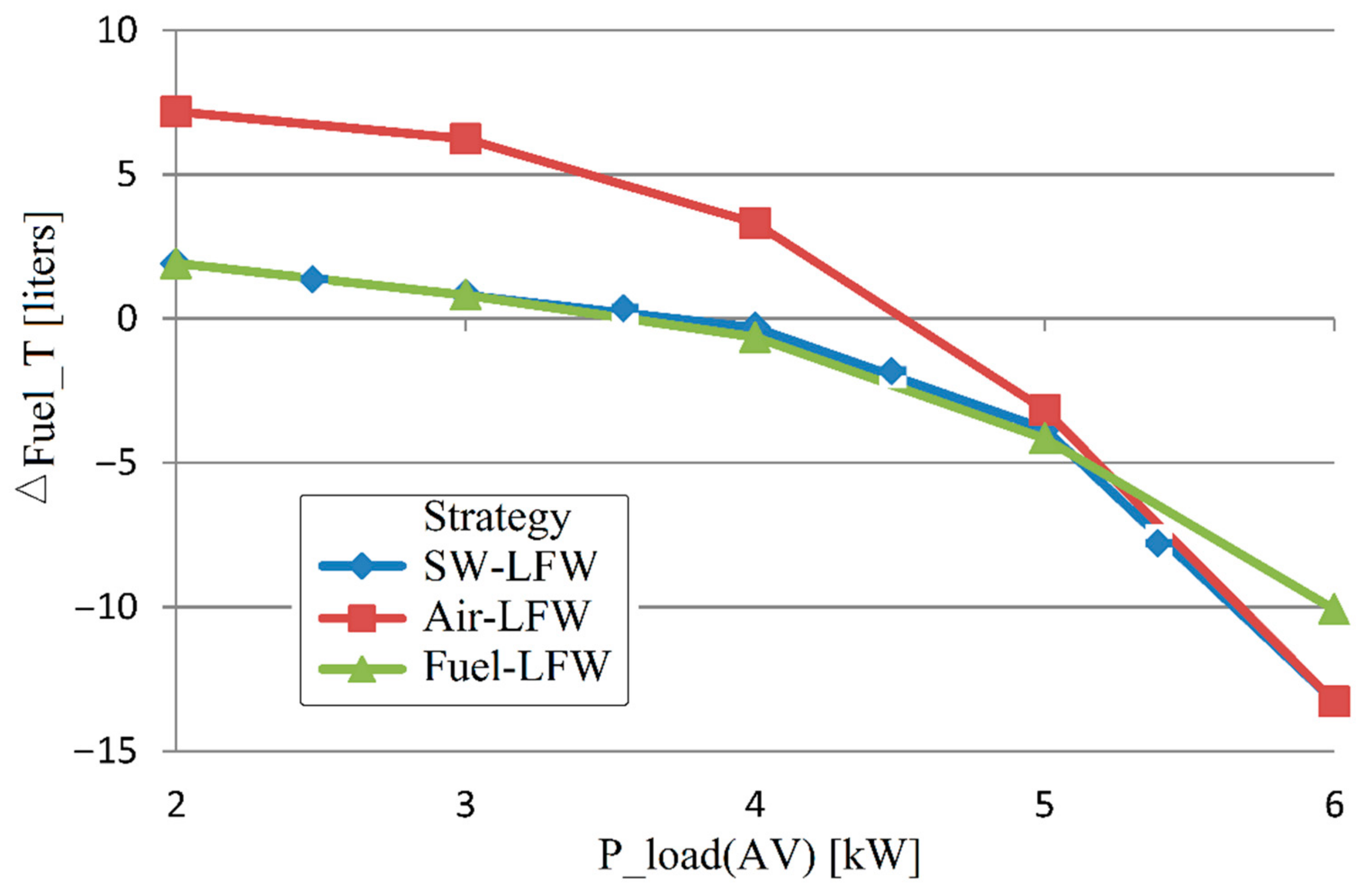
4.2.1. The First Variable Load Cycle with Different Power Pload(AV) Levels

The first variable load cycle with different Pload(AV) values was used to test the Air–LFW and Fuel–LFW strategies [110,111]. Therefore, this 12 s load cycle was also utilized in this work to estimate the fuel economy point of the SW–LFW technique. The power levels were 0.75·Pload(AV), 1.25·Pload(AV), and 1.00·Pload(AV), during 4 s for each level. Therefore, the average value (AV) of this 12 s load cycle was power Pload(AV). The values employed for Pload(AV) were 2, 3, 4, 5, and 6 kW (see Table 4) in order to operate the FC system within the admissible limit for FC power (up to 8 kW). For example, the power levels for the load cycle with power Pload(AV) = 6 kW were 4.5, 7.5, and 6 kW, the levels for the 4 kW load cycle were 3, 5, and 4 kW, and the levels for the 2 kW load cycle were 1.5, 2.5, and 2 kW.
If the threshold P r e f is selected in the middle of the range of these levels, 4   kW P r e f < 4.5   kW , then the SW–LFW technique performs as the Fuel–LFW technique for the load cycles with power Pload(AV) of 2 kW and Pload(AV) of 3 kW, as the Air–LFW technique for the load drive cycle with power Pload(AV) of 2 kW, and specifically for the load drive cycles with power Pload(AV) of 4 kW and power Pload(AV) of 5 kW, using the switching rules (24)–(26). This kind of operation for the SW–LFW strategy could be observed in Table 4, by analyzing the fuel economy recorded, and was easier observed in fuel economy in Figure 5.

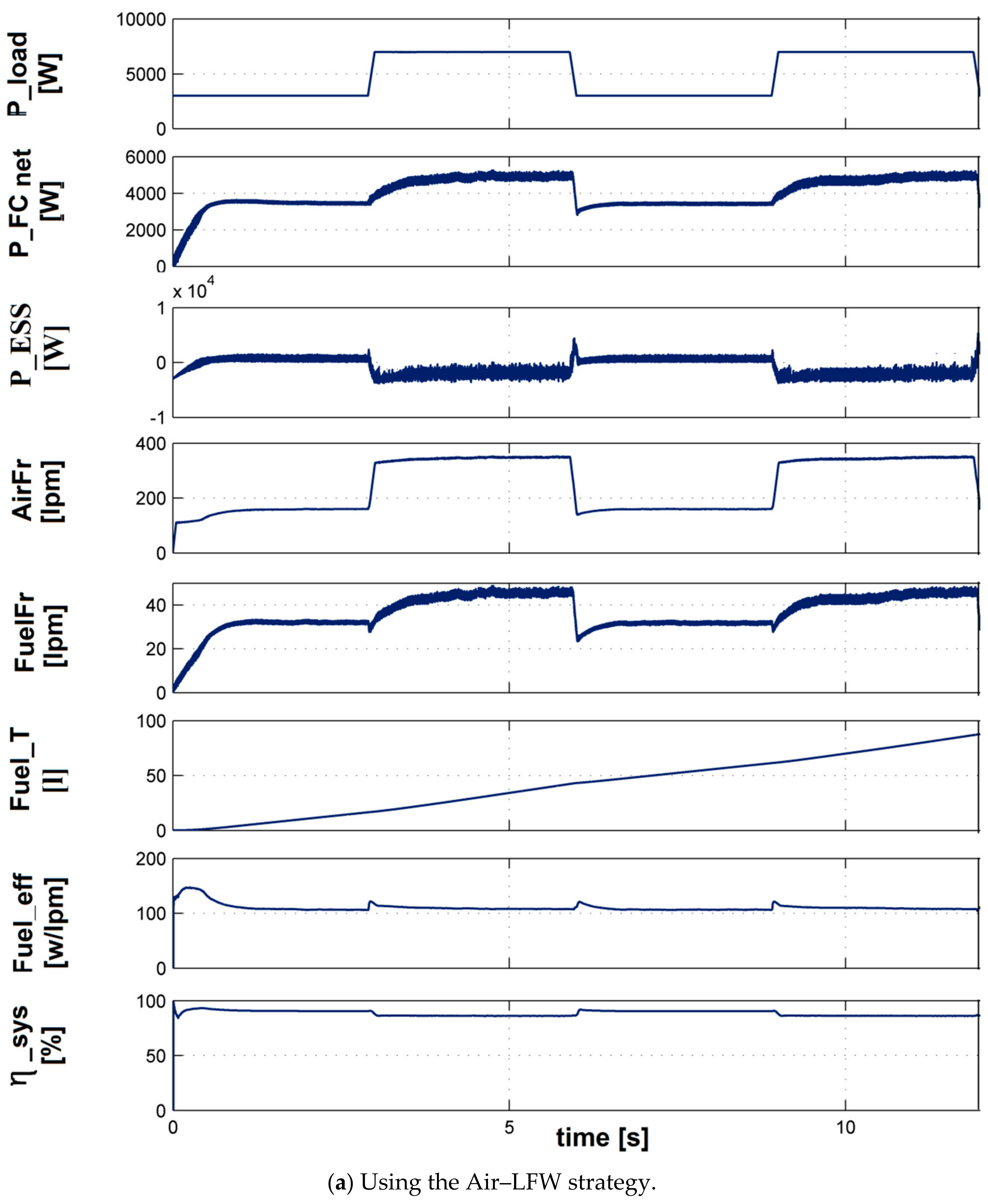
4.2.2. The Second Variable Load Cycle with 3/7 kW Load Pulses

The second load profile used power values of 7 kW and 3 kW during 3 s for each level, resulting in a pulsed load profile (see the first curve in Figure 6). Figure 6 presents the characteristics of the FCHPS under the second load profile for strategies Air–LFW (Figure 6a), Fuel–LFW (Figure 6b), and SW–LFW (Figure 6c), with the plots structured as follows—the 1st plot illustrates the 3/7 kW pulsed load profile; the 2nd and 3rd curves portray the ESS power ( P E S S ) and fuel cell net power ( P F C n e t ) and; the 4th and 5th curves display the fueling flow rates (FuelFr and AirFr); the 6th plot in Figure 6c represents the airflow rate (AirFr) in case of the strategy proposed in [110]; the total fuel utilization ( F u e l T ), the fuel consumption efficiency ( F u e l e f f ), and the fuel cell electrical efficiency ( η s y s =   P F C n e t /   P F C ) are shown in the last three curves.
It is worth mentioning the observations. (1) The load-following management mode operated the AirFr regulator (refer to the 4th curve in Figure 6a) or the FuelFr regulator (see the 5th plot in Figure 6b) if the Air–LFW technique or Fuel–LFW technique was used. (2) The optimization loop set I F C I r e f G E S for the FuelFr regulator (see the search of the optimum of the FuelFr in the 5th plot in Figure 6a) or the AirFr regulator (see the search of the optimum of the AirFr in the 4th plot in Figure 6b) if the Air–LFW technique or the Fuel–LFW technique was used. (3) The FC system supplied the requested load demand based on the load-following regulation mode designed using Equation (6), P F C g e n P l o a d M V / η b o o s t , therefore, the battery functions in the charge–sustained mode (refer to the 3rd curve in Figure 6). (4) The ultracapacitor bank transiently stabilizes the power equilibrium during the dynamic load (see the 3rd plot in Figure 6). (5) The fuel consumption efficiency ( F u e l e f f ) had values in the range of 95 to 140 W/lpm (refer to the 7th curve in Figure 6a,b, and 8th plot in Figure 6c). Therefore, the optimization terms k f u e l F u e l e f f and 0.5 P F C n e t have comparable values for kfuel = 25. (6) The FC electrical efficiency ( η s y s ) had values in the range of 85 to 94% (see the 8th plot in Figure 6a,b, and 9th plot in Figure 6c), therefore, a new optimization function f = η s y s + k f u e l F u e l e f f might be defined for excellent fuel economy using kfuel in the scale of 0.5 to 2 lpm/W. (7) The proposed strategy is safer than that analyzed in [110] (where the second optimization loop is not involved in setting the desired-points of the fueling regulators and thus some perturbation (spikes) might appear in the desired-points of the fueling regulators due to the switching control (see the spike in the 5th plot of Figure 6c, as compared to the 4th plot of Figure 6c, which appears when the set-points I r e f L F W and I F C + I r e f G E S 2 are switched [110], and the reference I F C + I r e f G E S 2 is clearly different from the reference I r e f L F W ).
It is important mentioning that when using the Air–LFW technique or the Fuel–LFW technique, such spikes do not appear in the fueling flow rated, because the fueling references ( I r e f F u e l = I F C and I r e f A i r = I r e f L F W for the Air–LFW technique, and I r e f A i r = I F C and I r e f F u e l = I r e f L F W for the Fuel–LFW technique) are based on the references I r e f L F W and I F C . The proposed strategy switches these references, but I F C I r e f L F W considering Equation (14).
The total fuel consumption is shown in the 6th curve of Figure 6a,b, and in the 7th plot of Figure 6c, and the fuel efficiency is shown in Table 5. Fuel economy for the SW–LFW technique, as compared to the sFF technique, represented around 25% of F u e l T s F F . The fuel efficiency for the SW–LFW technique as compared to the Air–LFW and Fuel–LFW techniques was 1.49-times and 2.38-times higher, respectively.
In the case of pulsed load, the threshold P r e f could be chosen between the levels, 3   kW < P r e f < 7   kW , but, considering the results for a constant load, it was obvious that the best value must be established for a variable load, based on a sensitivity analysis. For this, the third load profile (symmetrical stair up and down) was designed.

4.2.3. The Third Load Profile (Symmetrical Stair Up and Down)

The levels for the symmetrical stair were 3, 4, 5, 6, and 7 kW, with 2 s for each level in the stair up and other 2 s for each level in the stair down (see the first plot in Figure 8). The threshold P r e f was chosen between the levels, in order to analyze the fuel efficiency obtained in each case (see Table 6).
The best fuel efficiency for the SW–LFW technique compared to the sFF technique was observed for P r e f = 5.5   kW , at about 13.6% of F u e l T s F F (100 × 38.9/286.5 ≅ 13.58%). The fuel efficiency for the SW–LFW technique compared to the Air–LFW and Fuel–LFW techniques was 2.23- times and 2.47-times higher, respectively. Fuel economy using different values for the threshold P r e f is shown in Figure 7. The fuel efficiency utilizing the SW-FLW technique with power P r e f = 2.5   kW was equal to that gained utilizing the Air-FLW strategy, with small differences appearing due to the use of the Fuel-FLW strategy during the starting phase (until the load became higher than 2.5 kW).
It is worth mentioning that only minor differences appeared in the fuel economy obtained for different levels of the threshold P r e f using the SW–LFW technique, as compared to the switching technique proposed in [110] (see the last column of Table 6 and Figure 7). Thus, at the same fuel economy that might be obtained during a load cycle, the proposed strategy had the advantages of being simpler and safer than the switching strategy proposed in [110].
Figure 8 presents the behavior of the FCHPS under the second load profile for the strategies Air–LFW (Figure 8a), Fuel–LFW (Figure 8b), and SW–LFW (Figure 8c), with the plots structured as in Figure 6. Beside the above-mentioned findings for transient load, these further observations were of significance. (1) The search for the optimum using the Air–LFW or the SW–LFW strategies for P l o a d > P r e f = 4.5   kW is performed via the FuelFr regulator because I F C I r e f G E S ; because the optimization function was defined to minimize the fuel economy, the minimum values of the FuelFr is tracked (refer to the 5th plot in Figure 8a,c) and the FC power is different from the requested load. (2) This power difference (given by the power transfer balance on the DC distributed network) is sustained by the storage device (here a battery), which is charged or discharged during the load cycle, but the SOC remains the same at the end (see the 3th plot in Figure 8a). (3) The search for the optimum using the Fuel–LFW or the SW–LFW strategies for P l o a d < P r e f = 4.5   kW operates via the AirFr regulator, so the FuelFr controller is controlled using the load-following technique (see the 5th plot in Figure 8b); thus, the FC power is almost close to the requested load. (4) the battery storage device functions in a charge-sustained mode (refer to the 3rd curve in Figure 8b). (5) In the case of a dynamic load in the full range, the fuel efficiency for the Air–LFW and Fuel–LFW techniques seems to be the same (see Table 6); the difference of 1.7 L means about 0.63% of the total fuel utilization.
Additionally, it is worth mentioning the aforementioned spike when the references I r e f L F W and I F C + I r e f G E S 2 are switched [110] (refer to the 4th curve of Figure 8c).

5. Discussion and Next Works

The results obtained for the FCHPS in previous sections and [110] are summarized in Table 7, Table 8, Table 9 and Table 10, for the case of keff = 25 and Pref = 4.5 kW, where the fuel economy indicator was calculated for a given load profile using the relationship % F u e l T s t r a t e g y l o a d = 100   F u e l T r e f e r e n c e l o a d F u e l T s t r a t e g y l o a d F u e l T r e f e r e n c e l o a d .
Table 7 presents the percent of fuel economy for different constant Pload values (mentioned in the last column), highlighting that the SW–LFW strategy achieved the best fuel economy through the switching technique of the Air–LFW and Fuel–LFW strategies. The average value of the fuel economy percentages for the eight load levels was calculated using 1 8 P _ l o a d % F u e l T s t r a t e g y P _ l o a d . The value obtained showed that the SW–LFW strategy and the strategy proposed in [110] were of different classes (the first used a single GHG controller, the second used two GES controllers, which led to the expansion of the search field by using two variables and therefore better performance).
Better performance for the strategy proposed in [110] compared to the SW–LFW strategy proposed in this study was also obtained for a variable load profile but with low dynamics (note that the power levels used were 0.75·Pload(AV), 1.25·Pload(AV), and 1.00·Pload(AV) for the first load profile). Table 8 presents the percent of fuel economy for different first load profiles, mentioning the Pload(AV) values in the last column.
For a variable load profile with a dynamic across the full range of loads allowed, the performance indicator had similar values for the SW–LFW and SW strategies [110] (see percentage of fuel economy for the second and third load profile presented in Table 9 and Table 10).
A possible explanation would be that the load dynamics could no longer be tracked due to the limited search speed, to avoid fuel starvation, and the advantage of searching with two variables was lost. Although the discussion on the performance of the SW–LFW strategy remained open, as compared to the strategy proposed in [110], it was obvious that the current limitations imposed by the safe operation of the FC system limited the search speed. Therefore, the search slopes of maximum 100 A/s imposed in the air and fuel regulators limits the search speed and, in the end, similar performances are obtained (regardless of the search speed of the algorithm used). However, the advantage of the simplicity of the SW–LFW strategy still holds, as compared to the strategy proposed in [110].
The fuel consumption for the SW–LFW strategy, mentioned in Table 2 and Table 4, is shown in Figure 9 by load (a) and average load (b).
It is worth mentioning that the fuel consumption for the SW–LFW strategy was almost linear in both cases, the trend line depending on the load and the average load, according to the relations FuelT(SW) = 20.378 Pload + 14.868 and FuelT(SW) = 18.977 Pload(AV) + 14.323, respectively. Therefore, the fuel consumption could be estimated on the basis of the average load, up to the first refueling station on the planned road.
Consequently, the next works is focused on the following actions:
  • Testing the relationship between fuel consumption and average load for different load demand profiles.
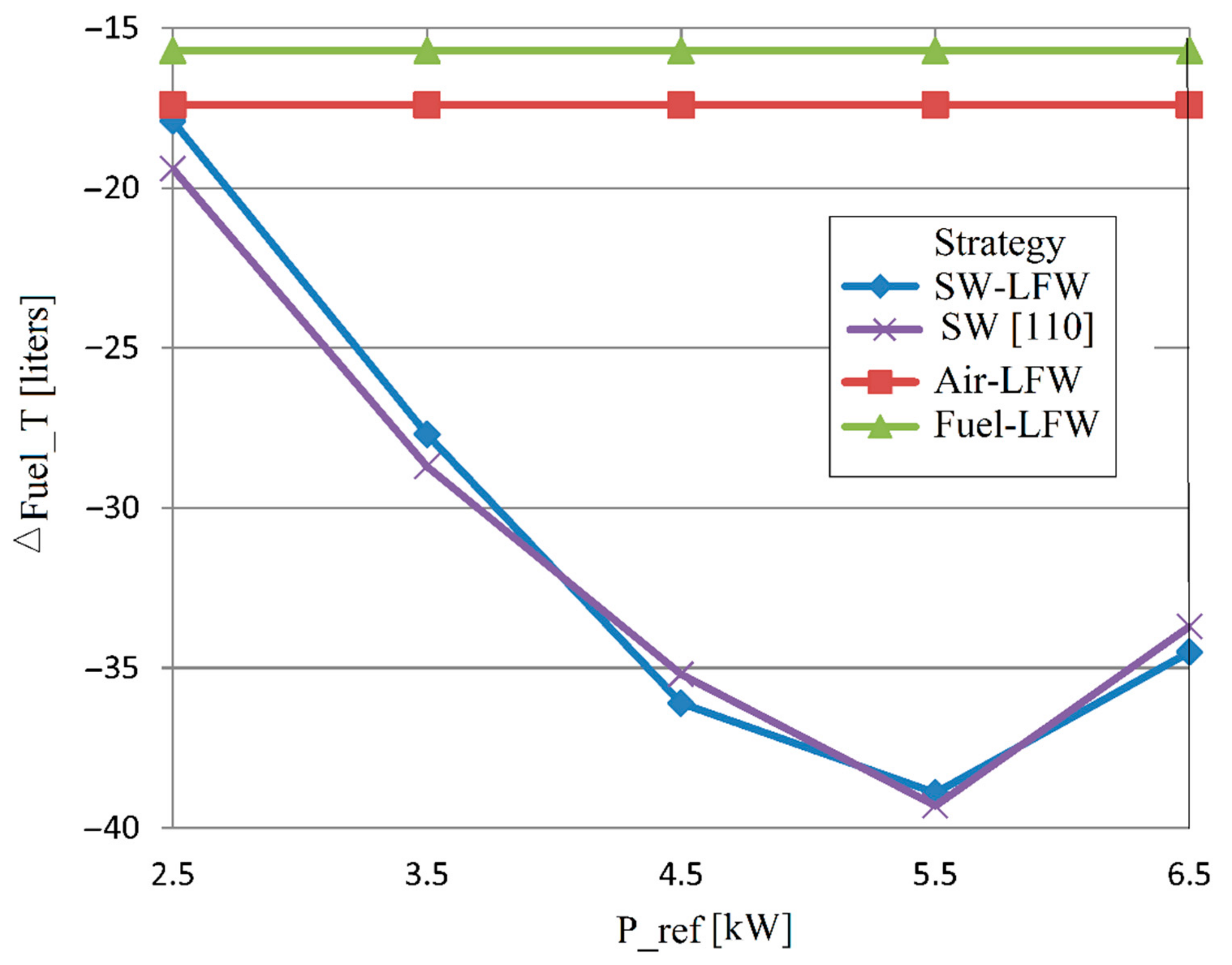
  • Finding the best threshold between the high and low loading ranges. This value of Pref = 4.5 kW was obtained on the basis of the sensitivity investigation functions for both variable and constant loads. The load-following management switches to the fuel and air regulators, if the load is higher or lower than this threshold. This value and other values close to this are to be considered for further tests under a different load profile.
  • Inclusion of a monitoring and energy management system for the battery. In this study, the system load demand was clearly sustained by the power supplied by the FC system and the battery storage device functions in a charge-sustained mode. Thus, the size of the battery might be reduced. Additionally, the battery’s life time increases by avoiding the charge–discharge cycles that appear in most strategies, based on SOC monitoring. An advanced energy management system [121,122] and a battery aging modeling [123,124] is to be included to evaluate the advantage of the LFW control over the battery life.
  • Reducing the number of switches of the fueling regulators’ references in the event of a high dynamic load. The SW–LFW strategy used a 200 W hysteresis controller (see Figure 3) instead of a simple comparator, to switch the reference I r e f L F W to the inputs of the fueling regulators ( I r e f F u e l and I r e f A i r ). Different values of the hysteresis band for the hysteresis controller is to be tested, in combination with an appropriate filtering of the load power.
In summary, besides the practical recommendations and next works mentioned above, the implementation of the SW–LFW strategy could be approached through the following step-by-step research methodology. (1) First, the strategies Air–LFW and Fuel–LFW must be tested for high and low load levels, using a simple searching algorithm and a Fuel Cell simulator based on a Hardware in the Loop Simulation (HILS) approach. (2) The air and fuel flow rates obtained with the techniques Air–LFW and Fuel–LFW is to be recorded in a look-up table to use for the SW–LFW strategy (a look-up table approach of the load-following control presented in this work). (3) The obtained fuel economy is to be validated on a Fuel Cell system using the SW–LFW strategy for variable load profiles. (4) The fuel efficiency should be improved by testing other thresholds, using recently developed searching algorithms (such as the Global Extremum Seeking algorithm used in this paper), the load-following management in place of the look-up table approach, faster searching algorithms than GES algorithm used here, etc.

6. Conclusions

This work analyzed the performance of the SW–LFW technique in comparison to strategies based on Air–LFW, Fuel–LFW, sFF control, and the switching strategy proposed in [110]. The fuel efficiency was better for the SW–LFW strategy in case of a dynamic load across the full range as it used the best strategy for a certain load level—Air–LFW strategy for high-load values and Fuel–LFW strategy for low-load values.
In addition, the fueling regulator, which was not controlled based on the load-following technique, was utilized to improve the fuel economy employing a real-time optimization loop.
In consequence, the key observations of this work were as follows. (1) A new energy management scheme based on the SW–LFW technique to further improve fuel economy compared to basic techniques (the Air–LFW and Fuel–LFW techniques) and sFF reference strategy. (2) SW–LFW strategy has the advantages of improved battery lifetime and reduced size, by switching the load-following control to the fueling controllers. (3) The fuel economy in case of a dynamic load across the full range was doubled compared to basic strategies (about 2.23-times and 2.47-times higher compared to Air–LFW and Fuel–LFW techniques, respectively). (4) The total fuel utilization was reduced by more than 13%, as compared to commercial strategy based on the sFF technique. (5) At the same fuel economy that could be obtained during a dynamic load cycle, the proposed strategy had the advantages of simplicity and safety in operation, as compared to the switching strategy proposed in [110]. (6) In addition, fuel consumption could be estimated based on the average load to the first refueling station on the planned road, using the linear relationship obtained in this study.
In conclusion, this study would help improve the performance of the FC vehicles, by utilizing the innovative solutions proposed in this paper.

Author Contributions

Research methodology, N.B.; writing—original draft preparation, N.B. and P.T.; supervision, P.T. and N.B.; Investigation, N.B. and P.T.; writing—review and editing, N.B. and P.T. All authors have read and agreed to the published version of the manuscript.

Funding

This work was partially supported by the International Research Partnerships: Electrical Engineering Thai-French Research Center (EE-TFRC) between King Mongkut’s University of Technology North Bangkok and University of Lorraine under Grant KMUTNB-64-KNOW-31.

Institutional Review Board Statement

Not applicable.

Informed Consent Statement

Not applicable.

Data Availability Statement

Not applicable.

Conflicts of Interest

The authors declare no conflict of interest.

References

  1. Gielen, D.; Boshell, F.; Saygin, D.; Bazilian, M.D.; Wagner, N.; Gorini, R. The role of renewable energy in the global energy transformation. Energy Strategy Rev. 2019, 24, 38–50. [Google Scholar] [CrossRef]
  2. Hesselink, L.X.W.; Chappin, E.J.L. Adoption of energy efficient technologies by households—Barriers, policies and agent-based modelling studies. Renew Sustain. Energy Rev. 2019, 99, 29–41. [Google Scholar] [CrossRef]
  3. Wang, F.-C.; Hsiao, Y.-S.; Yang, Y.-Z. The Optimization of Hybrid Power Systems with Renewable Energy and Hydrogen Generation. Energies 2018, 11, 1948. [Google Scholar] [CrossRef] [Green Version]
  4. Bukar, A.L.; Tan, C.W. A review on stand-alone photovoltaic-wind energy system with fuel cell: System optimization and energy management strategy. J. Clean. Prod. 2019, 221, 73–88. [Google Scholar] [CrossRef]
  5. Sulaiman, N.; Hannan, M.; Mohamed, A.; Ker, P.; Majlan, E.; Daud, W.W. Optimization of energy management system for fuel-cell hybrid electric vehicles: Issues and recommendations. Appl. Energy 2018, 228, 2061–2079. [Google Scholar] [CrossRef]
  6. Sorrentino, M.; Cirillo, V.; Nappi, L. Development of flexible procedures for co-optimizing design and control of fuel cell hybrid vehicles. Energy Convers. Manag. 2019, 185, 537–551. [Google Scholar] [CrossRef]
  7. Bizon, N. Hybrid power sources (HPSs) for space applications: Analysis of PEMFC/Battery/SMES HPS under unknown load containing pulses. Renew. Sustain. Energy Rev. 2019, 105, 14–37. [Google Scholar] [CrossRef]
  8. Pan, Z.; An, L.; Wen, C. Recent advances in fuel cells based propulsion systems for unmanned aerial vehicles. Appl. Energy 2019, 240, 473–485. [Google Scholar] [CrossRef]
  9. Bizon, N. Real-time optimization strategy for fuel cell hybrid power sources with load-following control of the fuel or air flow. Energy Convers. Manag. 2018, 157, 13–27. [Google Scholar] [CrossRef]
  10. Olatomiwa, L.; Mekhilef, S.; Ismail, M.; Moghavvemi, M. Energy management strategies in hybrid renewable energy systems: A review. Renew. Sustain. Energy Rev. 2016, 62, 821–835. [Google Scholar] [CrossRef]
  11. Bizon, N. Optimal Operation of Fuel Cell/Wind Turbine Hybrid Power System under Turbulent Wind and Variable Load. Appl. Energy 2018, 212, 196–209. [Google Scholar] [CrossRef]
  12. Priya, K.; Sathishkumar, K.; Rajasekar, N. A comprehensive review on parameter estimation techniques for Proton Exchange Membrane fuel cell modelling. Renew. Sustain. Energy Rev. 2018, 93, 121–144. [Google Scholar] [CrossRef]
  13. Yue, M.; Jemei, S.; Gouriveau, R.; Zerhouni, N. Review on health-conscious energy management strategies for fuel cell hybrid electric vehicles: Degradation models and strategies. Int. J. Hydrogen Energy 2019, 44, 6844–6861. [Google Scholar] [CrossRef]
  14. Bizon, N. Effective mitigation of the load pulses by controlling the battery/SMES hybrid energy storage system. Appl. Energy 2018, 229, 459–473. [Google Scholar] [CrossRef]
  15. Dafalla, A.M.; Jiang, J. Stresses and their impacts on proton exchange membrane fuel cells: A review. Int. J. Hydrogen Energy 2018, 43, 2327–2348. [Google Scholar] [CrossRef]
  16. Chen, H.; Zhao, X.; Zhang, T.; Pei, P. The reactant starvation of the proton exchange membrane fuel cells for vehicular applications: A review. Energy Convers. Manag. 2019, 182, 282–298. [Google Scholar] [CrossRef]
  17. Luo, Y.; Jiao, K. Cold start of proton exchange membrane fuel cell. Prog. Energy Combust. Sci. 2018, 64, 29–61. [Google Scholar] [CrossRef]
  18. Zhang, T.; Wang, P.; Chen, H.; Pei, P. A review of automotive proton exchange membrane fuel cell degradation under start-stop operating condition. Appl. Energy 2018, 223, 249–262. [Google Scholar] [CrossRef]
  19. Dijoux, E.; Steiner, N.Y.; Benne, M.; Péra, M.-C.; Pérez, B.G. A review of fault tolerant control strategies applied to proton exchange membrane fuel cell systems. J. Power Sources 2017, 359, 119–133. [Google Scholar] [CrossRef] [Green Version]
  20. Das, V.; Padmanaban, S.; Venkitusamy, K.; Selvamuthukumaran, R.; Blaabjerg, F.; Siano, P. Recent advances and challenges of fuel cell based power system architectures and control—A review. Renew. Sustain. Energy Rev. 2017, 73, 10–18. [Google Scholar] [CrossRef]
  21. Bizon, N. Load-following mode control of a standalone renewable/fuel cell hybrid power source. Energy Convers. Manag. 2014, 77, 763–772. [Google Scholar] [CrossRef]
  22. Daud, W.; Rosli, R.; Majlan, E.; Hamid, S.; Mohamed, R.; Husaini, T. PEM fuel cell system control: A review. Renew. Energy 2017, 113, 620–638. [Google Scholar] [CrossRef]
  23. Bizon, N.; Radut, M.; Oproescu, M. Energy control strategies for the Fuel Cell Hybrid Power Source under unknown load profile. Energy 2015, 86, 31–41. [Google Scholar] [CrossRef]
  24. Ahmadi, P.; Torabi, S.H.; Afsaneh, H.; Sadegheih, Y.; Ganjehsarabi, H.; Ashjaee, M. The effects of driving patterns and PEM fuel cell degradation on the lifecycle assessment of hydrogen fuel cell vehicles. Int. J. Hydrogen Energy 2020, 45, 3595–3608. [Google Scholar] [CrossRef]
  25. Wang, F.-C.; Lin, K.-M. Impacts of Load Profiles on the Optimization of Power Management of a Green Building Employing Fuel Cells. Energies 2018, 12, 57. [Google Scholar] [CrossRef] [Green Version]
  26. Zhao, D.; Xu, L.; Huangfu, Y.; Dou, M.; Liu, J. Semi-physical modeling and control of a centrifugal compressor for the air feeding of a PEM fuel cell. Energy Convers. Manag. 2017, 154, 380–386. [Google Scholar] [CrossRef]
  27. Han, J.; Yu, S. Ram air compensation analysis of fuel cell vehicle cooling system under driving modes. Appl. Therm. Eng. 2018, 142, 530–542. [Google Scholar] [CrossRef]
  28. Zhang, H.; Li, X.; Liu, X.; Yan, J. Enhancing fuel cell durability for fuel cell plug-in hybrid electric vehicles through strategic power management. Appl. Energy 2019, 241, 483–490. [Google Scholar] [CrossRef]
  29. Pukrushpan, J.T.; Stefanopoulou, A.G.; Peng, H. Control of fuel cell breathing. IEEE Control Syst. Mag. 2004, 24, 30–46. [Google Scholar]
  30. Ahn, J.-W.; Choe, S.-Y. Coolant controls of a PEM fuel cell system. J. Power Sources 2008, 179, 252–264. [Google Scholar] [CrossRef]
  31. Beirami, H.; Shabestari, A.Z.; Zerafat, M.M. Optimal PID plus fuzzy controller design for a PEM fuel cell air feed system using the self-adaptive differential evolution algorithm. Int. J. Hydrogen Energy 2015, 40, 9422–9434. [Google Scholar] [CrossRef]
  32. Liu, Z.; Li, L.; Ding, Y.; Deng, H.; Chen, W. Modeling and control of an air supply system for a heavy duty PEMFC engine. Int. J. Hydrogen Energy 2016, 41, 16230–16239. [Google Scholar] [CrossRef]
  33. Talj, R.; Ortega, R.; Astolfi, A. Passivity and robust PI control of the air supply system of a PEM fuel cell model. Automatica 2011, 47, 2554–2561. [Google Scholar] [CrossRef]
  34. Cano, M.H.; Mousli, M.I.A.; Kelouwani, S.; Agbossou, K.; Hammoudi, M.; Dubéc, Y. Improving a free air breathing proton exchange membrane fuel cell through the Maximum Efficiency Point Tracking method. J. Power Sources 2017, 345, 264–274. [Google Scholar] [CrossRef]
  35. Baroud, Z.; Benmiloud, M.; Benalia, A.; Ocampo-Martinez, C. Novel hybrid fuzzy-PID control scheme for air supply in PEM fuel-cell-based systems. Int. J. Hydrogen Energy 2017, 42, 10435–10447. [Google Scholar] [CrossRef] [Green Version]
  36. Hasikos, J.; Sarimveis, H.; Zervas, P.; Markatos, N. Operational optimization and real-time control of fuel-cell systems. J. Power Sources 2009, 193, 258–268. [Google Scholar] [CrossRef]
  37. Nejad, H.C.; Farshad, M.; Gholamalizadeh, E.; Askarian, B.; Akbarimajd, A. A novel intelligent-based method to control the output voltage of Proton Exchange Membrane Fuel Cell. Energy Convers. Manag. 2019, 185, 455–464. [Google Scholar] [CrossRef]
  38. Arce, A.; Alejandro, J.; Bordons, C.; Daniel, R. Real-time implementation of a constrained MPC for efficient airflow control in a PEM fuel cell. IEEE Trans. Ind. Electron. 2010, 57, 1892–1905. [Google Scholar] [CrossRef]
  39. Ziogou, C.; Papadopoulou, S.; Pistikopoulos, E.; Georgiadis, M.; Voutetakis, S. Model-Based Predictive Control of Integrated Fuel Cell Systems—From Design to Implementation. Adv. Energy Syst. Eng. 2016, 2017, 387–430. [Google Scholar] [CrossRef]
  40. Ziogou, C.; Papadopoulou, S.; Georgiadis, M.C.; Voutetakis, S. On-line nonlinear model predictive control of a PEM fuel cell system. J. Process. Control. 2013, 23, 483–492. [Google Scholar] [CrossRef]
  41. Barzegari, M.M.; Alizadeh, E.; Pahnabi, A.H. Grey-box modeling and model predictive control for cascade-type PEMFC. Energy 2017, 127, 611–622. [Google Scholar] [CrossRef]
  42. Ziogou, C.; Voutetakis, S.; Georgiadis, M.C.; Papadopoulou, S. Model predictive control (MPC) strategies for PEM fuel cell systems—A comparative experimental demonstration. Chem. Eng. Res. Des. 2018, 131, 656–670. [Google Scholar] [CrossRef]
  43. Laghrouche, S.; Harmouche, M.; Ahmed, F.S.; Chitour, Y. Control of PEMFC Air-Feed System Using Lyapunov-Based Robust and Adaptive Higher Order Sliding Mode Control. IEEE Trans. Control. Syst. Technol. 2014, 23, 1. [Google Scholar] [CrossRef] [Green Version]
  44. Pilloni, A.; Pisano, A.; Usai, E. Observer-Based Air Excess Ratio Control of a PEM Fuel Cell System via High-Order Sliding Mode. IEEE Trans. Ind. Electron. 2015, 62, 5236–5246. [Google Scholar] [CrossRef] [Green Version]
  45. Deng, H.; Li, Q.; Chen, W.; Zhang, G. High-Order Sliding Mode Observer Based OER Control for PEM Fuel Cell Air-Feed System. IEEE Trans. Energy Convers. 2017, 33, 232–244. [Google Scholar] [CrossRef]
  46. Sankar, K.; Jana, A.K. Nonlinear multivariable sliding mode control of a reversible PEM fuel cell integrated system. Energy Convers. Manag. 2018, 171, 541–565. [Google Scholar] [CrossRef]
  47. Deng, H.; Li, Q.; Cui, Y.; Zhu, Y.; Chen, W. Nonlinear controller design based on cascade adaptive sliding mode control for PEM fuel cell air supply systems. Int. J. Hydrogen Energy 2019, 44, 19357–19369. [Google Scholar] [CrossRef]
  48. Saadi, R.; Kraa, O.; Ayad, M.; Becherif, M.; Ghodbane, H.; Bahri, M.; Aboubou, A. Dual loop controllers using PI, sliding mode and flatness controls applied to low voltage converters for fuel cell applications. Int. J. Hydrogen Energy 2016, 41, 19154–19163. [Google Scholar] [CrossRef]
  49. Derbeli, M.; Farhat, M.; Barambones, O.; Sbita, L. Control of PEM fuel cell power system using sliding mode and super-twisting algorithms. Int. J. Hydrogen Energy 2017, 42, 8833–8844. [Google Scholar] [CrossRef]
  50. Kunusch, C.; Puleston, P.F.; Mayosky, M.A.; Riera, J. Sliding Mode Strategy for PEM Fuel Cells Stacks Breathing Control Using a Super-Twisting Algorithm. IEEE Trans. Control. Syst. Technol. 2008, 17, 167–174. [Google Scholar] [CrossRef] [Green Version]
  51. Hernández-Torres, D.; Riu, D.; Sename, O. Reduced-order Robust Control of a Fuel Cell Air Supply System. IFAC-PapersOnLine 2017, 50, 96–101. [Google Scholar] [CrossRef]
  52. Sun, J.; Kolmanovsky, I. Load governor for fuel cell oxygen starvation protection: A robust nonlinear reference governor approach. IEEE Trans. Contr. Syst. Technol. 2005, 13, 911–920. [Google Scholar]
  53. Han, J.; Yu, S.; Yi, S. Adaptive control for robust air flow management in an automotive fuel cell system. Appl. Energy 2017, 190, 73–83. [Google Scholar] [CrossRef]
  54. He, Y.; Xing, L.; Zhang, Y.; Zhang, J.; Cao, F.; Xing, Z. Development and experimental investigation of an oil-free twin-screw air compressor for fuel cell systems. Appl. Therm. Eng. 2018, 145, 755–762. [Google Scholar] [CrossRef]
  55. Li, Q.; Chen, W.; Liu, Z.; Guo, A.; Liu, S. Control of proton exchange membrane fuel cell system breathing based on maximum net power control strategy. J. Power Sources 2013, 241, 212–218. [Google Scholar] [CrossRef]
  56. Mane, S.; Mejari, M.; Kazi, F.; Singh, N. Improving Lifetime of Fuel Cell in Hybrid Energy Management System by Lure–Lyapunov-Based Control Formulation. IEEE Trans. Ind. Electron. 2017, 64, 6671–6679. [Google Scholar] [CrossRef]
  57. Ramos-Paja, C.A.; Spagnuolo, G.; Petrone, G.; Mamarelis, E. A perturbation strategy for fuel consumption minimization in polymer electrolyte membrane fuel cells: Analysis, Design and FPGA implementation. Appl. Energy 2014, 119, 21–32. [Google Scholar] [CrossRef]
  58. Bizon, N.; Lopez-Guede, J.M.; Kurt, E.; Thounthong, P.; Mazare, A.G.; Ionescu, L.M.; Iana, G. Hydrogen economy of the fuel cell hybrid power system optimized by air flow control to mitigate the effect of the uncertainty about available renewable power and load dynamics. Energy Convers. Manag. 2019, 179, 152–165. [Google Scholar] [CrossRef]
  59. Pukrushpan, J.T.; Stefanopoulou, A.G.; Peng, H. Control of Fuel Cell Power Systems; Springer International Publishing: New York, NY, USA, 2004. [Google Scholar]
  60. Zhong, D.; Lin, R.; Liu, D.; Cai, X. Structure optimization of anode parallel flow field for local starvation of proton exchange membrane fuel cell. J. Power Sources 2018, 403, 1–10. [Google Scholar] [CrossRef]
  61. Hong, L.; Chen, J.; Liu, Z.; Huang, L.; Wu, Z. A nonlinear control strategy for fuel delivery in PEM fuel cells considering nitrogen permeation. Int. J. Hydrogen Energy 2017, 42, 1565–1576. [Google Scholar] [CrossRef]
  62. Bao, C.; Ouyang, M.; Yi, B. Modeling and control of air stream and hydrogen flow with recirculation in a PEM fuel cell system—I. Control-oriented modeling. Int. J. Hydrogen Energy 2006, 31, 1879–1896. [Google Scholar] [CrossRef]
  63. Bao, C.; Ouyang, M.; Yi, B. Modeling and control of air stream and hydrogen flow with recirculation in a PEM fuel cell system—II. Linear and adaptive nonlinear control. Int. J. Hydrogen Energy 2006, 31, 1897–1913. [Google Scholar] [CrossRef]
  64. He, J.; Choe, S.-Y.; Hong, C.-O. Analysis and control of a hybrid fuel delivery system for a polymer electrolyte membrane fuel cell. J. Power Sources 2008, 185, 973–984. [Google Scholar] [CrossRef]
  65. He, J.; Ahn, J.; Choe, S.-Y. Analysis and control of a fuel delivery system considering a two-phase anode model of the polymer electrolyte membrane fuel cell stack. J. Power Sources 2011, 196, 4655–4670. [Google Scholar] [CrossRef]
  66. Thounthong, P.; Mungporn, P.; Pierfederici, S.; Guilbert, D.; Bizon, N. Adaptive Control of Fuel Cell Converter Based on a New Hamiltonian Energy Function for Stabilizing the DC Bus in DC Microgrid Applications. Mathematics 2020, 8, 2035. [Google Scholar] [CrossRef]
  67. Luna, J.; Ocampo-Martinez, C.; Serra, M. Nonlinear predictive control for the concentrations profile regulation under unknown reaction disturbances in a fuel cell anode gas channel. J. Power Sources 2015, 282, 129–139. [Google Scholar] [CrossRef] [Green Version]
  68. Park, G.; Gajic, Z. A Simple Sliding Mode Controller of a Fifth-Order Nonlinear PEM Fuel Cell Model. IEEE Trans. Energy Convers. 2013, 29, 65–71. [Google Scholar] [CrossRef]
  69. Matraji, I.; Laghrouche, S.; Jemei, S.; Wack, M. Robust control of the PEM fuel cell air-feed system via sub-optimal second order sliding mode. Appl. Energy 2013, 104, 945–957. [Google Scholar] [CrossRef]
  70. Baik, K.D.; Kim, M.S. Characterization of nitrogen gas crossover through the membrane in proton-exchange membrane fuel cells. Int. J. Hydrogen Energy 2011, 36, 732–739. [Google Scholar] [CrossRef]
  71. Steinberger, M.; Geiling, J.; Oechsner, R.; Frey, L. Anode recirculation and purge strategies for PEM fuel cell operation with diluted hydrogen feed gas. Appl. Energy 2018, 232, 572–582. [Google Scholar] [CrossRef]
  72. Chen, Y.-S.; Yang, C.-W.; Lee, J.-Y. Implementation and evaluation for anode purging of a fuel cell based on nitrogen concentration. Appl. Energy 2014, 113, 1519–1524. [Google Scholar] [CrossRef]
  73. Piffard, M.; Gerard, M.; Bideaux, E.; Da Fonseca, R.; Massioni, P. Control by state observer of PEMFC anodic purges in dead-end operating mode. IFAC-PapersOnLine 2015, 48, 237–243. [Google Scholar] [CrossRef]
  74. Rabbani, A.; Rokni, M. Effect of nitrogen crossover on purging strategy in PEM fuel cell systems. Appl. Energy 2013, 111, 1061–1070. [Google Scholar] [CrossRef] [Green Version]
  75. Mahoney, F.M. Reduction-Oxidation Tolerant Electrodes for Solid Oxide Fuel Cells. U.S. Patent 20,100,159,356, 24 June 2010. [Google Scholar]
  76. Ahluwalia, R.; Wang, X. Buildup of nitrogen in direct hydrogen polymer-electrolyte fuel cell stacks. J. Power Sources 2007, 171, 63–71. [Google Scholar] [CrossRef]
  77. Pan, T.; Shen, J.; Sun, L.; Lee, K.Y. Thermodynamic modelling and intelligent control of fuel cell anode purge. Appl. Therm. Eng. 2019, 154, 196–207. [Google Scholar] [CrossRef]
  78. Koski, P.; Perez, L.C.; Ihonen, J. Comparing Anode Gas Recirculation with Hydrogen Purge and Bleed in a Novel PEMFC Laboratory Test Cell Configuration. Fuel Cells 2015, 15, 494–504. [Google Scholar] [CrossRef]
  79. Promislow, K.; St-Pierre, J.; Wetton, B. A simple, analytic model of polymer electrolyte membrane fuel cell anode recirculation at operating power including nitrogen crossover. J. Power Sources 2011, 196, 10050–10056. [Google Scholar] [CrossRef]
  80. Taghiabadi, M.M.; Zhiani, M. Degradation analysis of dead-ended anode PEM fuel cell at the low and high thermal and pressure conditions. Int. J. Hydrogen Energy 2019, 44, 4985–4995. [Google Scholar] [CrossRef]
  81. Yang, Y.; Zhang, X.; Guo, L.; Liu, H. Overall and local effects of operating conditions in PEM fuel cells with dead-ended anode. Int. J. Hydrogen Energy 2017, 42, 4690–4698. [Google Scholar] [CrossRef] [Green Version]
  82. Pérez, L.C.; Rajala, T.; Ihonen, J.; Koski, P.; Sousa, J.M.; Mendes, A. Development of a methodology to optimize the air bleed in PEMFC systems operating with low quality hydrogen. Int. J. Hydrogen Energy 2013, 38, 16286–16299. [Google Scholar] [CrossRef]
  83. Mahjoubi, C.; Olivier, J.-C.; Skander-Mustapha, S.; Machmoum, M.; Slama-Belkhodja, I. An improved thermal control of open cathode proton exchange membrane fuel cell. Int. J. Hydrogen Energy 2019, 44, 11332–11345. [Google Scholar] [CrossRef]
  84. Strahl, S.; Costa-Castelló, R. Temperature control of open-cathode PEM fuel cells. IFAC-PapersOnLine 2017, 50, 11088–11093. [Google Scholar] [CrossRef] [Green Version]
  85. Chang, Y.; Qin, Y.; Yin, Y.; Zhang, J.; Li, X. Humidification strategy for polymer electrolyte membrane fuel cells—A review. Appl. Energy 2018, 230, 643–662. [Google Scholar] [CrossRef]
  86. Liu, Z.; Chen, J.; Chen, S.; Huang, L.; Shao, Z. Modeling and Control of Cathode Air Humidity for PEM Fuel Cell Systems. IFAC-PapersOnLine 2017, 50, 4751–4756. [Google Scholar] [CrossRef]
  87. Bizon, N.; Thounthong, P. Real-time strategies to optimize the fueling of the fuel cell hybrid power source: A review of issues, challenges and a new approach. Renew. Sustain. Energy Rev. 2018, 91, 1089–1102. [Google Scholar] [CrossRef]
  88. Ou, K.; Yuan, W.-W.; Choi, M.; Yang, S.; Kim, Y.-B. Performance increase for an open-cathode PEM fuel cell with humidity and temperature control. Int. J. Hydrogen Energy 2017, 42, 29852–29862. [Google Scholar] [CrossRef]
  89. Ahn, J.-W.; He, J.; Choe, S.-Y. Design of Air, Water, Temperature and Hydrogen Controls for a PEM Fuel Cell System. In Proceedings of the ASME 2011 9th International Conference on Fuel Cell Science, Engineering and Technology, Washington, DC, USA, 7–10 August 2011; pp. 711–718. Available online: https://asmedigitalcollection.asme.org/FUELCELL/proceedings-abstract/FUELCELL2011/54693/711/357956 (accessed on 9 February 2021).
  90. Bizon, N. Energy optimization of fuel cell system by using global extremum seeking algorithm. Appl. Energy 2017, 206, 458–474. [Google Scholar] [CrossRef]
  91. Sorlei, I.-S.; Bizon, N.; Thounthong, P.; Varlam, M.; Carcadea, E.; Culcer, M.; Iliescu, M.; Raceanu, M. Fuel Cell Electric Vehicles—A Brief Review of Current Topologies and Energy Management Strategies. Energies 2021, 14, 252. [Google Scholar] [CrossRef]
  92. Bizon, N.; Mazare, A.G.; Ionescu, L.M.; Enescu, F.M. Optimization of the proton exchange membrane fuel cell hybrid power system for residential buildings. Energy Convers. Manag. 2018, 163, 22–37. [Google Scholar] [CrossRef]
  93. Bizon, N. Nonlinear control of fuel cell hybrid power sources: Part II—Current control. Appl. Energy 2011, 88, 2574–2591. [Google Scholar] [CrossRef]
  94. Kaya, K.; Hames, Y. Two new control strategies: For hydrogen fuel saving and extend the life cycle in the hydrogen fuel cell vehicles. Int. J. Hydrogen Energy 2019, 44, 18967–18980. [Google Scholar] [CrossRef]
  95. Wang, Y.; Sun, Z.; Chen, Z. Rule-based energy management strategy of a lithium-ion battery, supercapacitor and PEM fuel cell system. Energy Procedia 2019, 158, 2555–2560. [Google Scholar] [CrossRef]
  96. Li, G.; Zhang, J.; He, H. Battery SOC constraint comparison for predictive energy management of plug-in hybrid electric bus. Appl. Energy 2017, 194, 578–587. [Google Scholar] [CrossRef]
  97. Torreglosa, J.P.; Garcia, P.; Fernandez, L.M.; Jurado, F. Predictive Control for the Energy Management of a Fuel-Cell–Battery–Supercapacitor Tramway. IEEE Trans. Ind. Inform. 2014, 10, 276–285. [Google Scholar] [CrossRef]
  98. Li, Q.; Wang, T.; Dai, C.; Chen, W.; Ma, L. Power Management Strategy Based on Adaptive Droop Control for a Fuel Cell-Battery-Supercapacitor Hybrid Tramway. IEEE Trans. Veh. Technol. 2017, 67, 5658–5670. [Google Scholar] [CrossRef]
  99. Ameur, K.; Hadjaissa, A.; Cheikh, M.S.A.; Cheknane, A.; Essounbouli, N. Fuzzy energy management of hybrid renewable power system with the aim to extend component lifetime. Int. J. Energy Res. 2017, 41, 1867–1879. [Google Scholar] [CrossRef]
  100. Ahmadi, S.; Bathaee, S.; Hosseinpour, A.H. Improving fuel economy and performance of a fuel-cell hybrid electric vehicle (fuel-cell, battery, and ultra-capacitor) using optimized energy management strategy. Energy Convers. Manag. 2018, 160, 74–84. [Google Scholar] [CrossRef]
  101. Zhou, D.; Al-Durra, A.; Gao, F.; Ravey, A.; Matraji, I.; Simões, M.G. Online energy management strategy of fuel cell hybrid electric vehicles based on data fusion approach. J. Power Sources 2017, 366, 278–291. [Google Scholar] [CrossRef]
  102. Bizon, N.; Thounthong, P. Fuel economy using the global optimization of the Fuel Cell Hybrid Power Systems. Energy Convers. Manag. 2018, 173, 665–678. [Google Scholar] [CrossRef]
  103. Fares, D.; Chedid, R.; Panik, F.; Karaki, S.; Jabr, R. Dynamic programming technique for optimizing fuel cell hybrid vehicles. Int. J. Hydrogen Energy 2015, 40, 7777–7790. [Google Scholar] [CrossRef]
  104. Onori, S.; Tribioli, L. Adaptive Pontryagin’s Minimum Principle supervisory controller design for the plug-in hybrid GM Chevrolet Volt. Appl. Energy 2015, 147, 224–234. [Google Scholar] [CrossRef]
  105. Bizon, N.; Hoarcă, I.C. Hydrogen saving through optimized control of both fueling flows of the Fuel Cell Hybrid Power System under a variable load demand and an unknown renewable power profile. Energy Convers. Manag. 2019, 184, 1–14. [Google Scholar] [CrossRef]
  106. Ramos-Paja, C.A.; Bordons, C.; Romero, A.; Giral, R.; Martinez-Salamero, L. Minimum Fuel Consumption Strategy for PEM Fuel Cells. IEEE Trans. Ind. Electron. 2008, 56, 685–696. [Google Scholar] [CrossRef]
  107. Ou, K.; Yuan, W.-W.; Choi, M.; Yang, S.; Jung, S.; Kim, Y.-B. Optimized power management based on adaptive-PMP algorithm for a stationary PEM fuel cell/battery hybrid system. Int. J. Hydrogen Energy 2018, 43, 15433–15444. [Google Scholar] [CrossRef]
  108. Bizon, N. Real-time optimization strategies of Fuel Cell Hybrid Power Systems based on Load-following control: A new strategy, and a comparative study of topologies and fuel economy obtained. Appl. Energy 2019, 241, 444–460. [Google Scholar] [CrossRef]
  109. Wang, Y.-X.; Kai, O.; Kim, Y.-B. Power source protection method for hybrid polymer electrolyte membrane fuel cell/lithiumion battery system. Renew. Energy 2017, 111, 381–391. [Google Scholar] [CrossRef]
  110. Bizon, N. Fuel saving strategy using real-time switching of the fueling regulators in the proton exchange membrane fuel cell system. Appl. Energy 2019, 252, 113449. [Google Scholar] [CrossRef]
  111. Bizon, N.; Culcer, M.; Oproescu, M.; Iana, G.; Laurentiu, I.; Mazare, A.; Iliescu, M. Real-time strategy to optimize the airflow rate of fuel cell hybrid power source under variable load cycle. In Proceedings of the 2017 International Conference on Applied Electronics, Pilsen, Czech Republic, 5–7 September 2017. [Google Scholar]
  112. Bizon, N. Sensitivity analysis of the fuel economy strategy for a fuel cell hybrid power system using fuel optimization and load-following based on air control. Energy Convers. Manag. 2019, 199, 111946. [Google Scholar] [CrossRef]
  113. Bizon, N.; Stan, V.A.; Cormos, A.C. Stan Optimization of the Fuel Cell Renewable Hybrid Power System using the Control Mode of the Required Load Power on the DC Bus. Energies 2019, 12, 1889. [Google Scholar] [CrossRef] [Green Version]
  114. Bizon, N.; Mazare, A.G.; Ionescu, L.M.; Thounthong, P.; Kurt, E.; Oproescu, M.; Serban, G.; Lita, I. Better Fuel Economy by Optimizing Airflow of the Fuel Cell Hybrid Power Systems Using Fuel Flow-Based Load-Following Control. Energies 2019, 12, 2792. [Google Scholar] [CrossRef] [Green Version]
  115. Bizon, N. Efficient fuel economy strategies for the Fuel Cell Hybrid Power Systems under variable renewable/load power profile. Appl. Energy 2019, 251, 113400. [Google Scholar] [CrossRef]
  116. Bizon, N. Sensitivity analysis of the fuel economy strategy based on load-following control of the fuel cell hybrid power system. Energy Convers. Manag. 2019, 199, 111946. [Google Scholar] [CrossRef]
  117. SimPowerSystems; Hydro-Québec and the MathWorks, Inc.: Natick, MA, USA, 2010; Available online: http://www.hydroquebec.com/innovation/en/pdf/2010G080-04A-SPS.pdf (accessed on 9 February 2021).
  118. Ettihir, K.; Boulon, L.; Agbossou, K. Optimization-based energy management strategy for a fuel cell/battery hybrid power system. Appl. Energy 2016, 163, 142–153. [Google Scholar] [CrossRef]
  119. Bizon, N.; Kurt, E. Performance analysis of the tracking of the global extreme on multimodal patterns using the Asymptotic Perturbed Extremum Seeking Control scheme. Int. J. Hydrogen Energy 2017, 42, 17645–17654. [Google Scholar] [CrossRef]
  120. Bizon, N.; Thounthong, P.; Raducu, M.; Constantinescu, L.M. Designing and modelling of the asymptotic perturbed extremum seeking control scheme for tracking the global extreme. Int. J. Hydrogen Energy 2017, 42, 17632–17644. [Google Scholar] [CrossRef]
  121. Wu, J.; Wei, Z.; Li, W.; Wang, Y.; Li, Y.; Sauer, D. Battery Thermal- and Health-Constrained Energy Management for Hybrid Electric Bus based on Soft Actor-Critic DRL Algorithm. IEEE Trans. Ind. Inform. 2021, 1. [Google Scholar] [CrossRef]
  122. Wu, J.; Wei, Z.; Liu, K.; Quan, Z.; Li, Y. Battery-Involved Energy Management for Hybrid Electric Bus Based on Expert-Assistance Deep Deterministic Policy Gradient Algorithm. IEEE Trans. Veh. Technol. 2020, 69, 12786–12796. [Google Scholar] [CrossRef]
  123. Wei, Z.; He, H.; Pou, J.; Tsui, K.-L.; Quan, Z.; Li, Y. Signal-Disturbance Interfacing Elimination for Unbiased Model Parameter Identification of Lithium-Ion Battery. IEEE Trans. Ind. Inform. 2020, 1. [Google Scholar] [CrossRef]
  124. Wei, Z.; Zhao, J.; He, H.; Ding, G.; Cui, H.; Liu, L. Future smart battery and management: Advanced sensing from external to embedded multi-dimensional measurement. J. Power Sources 2021, 489, 229462. [Google Scholar] [CrossRef]
Figure 1. Fuel cell hybrid power system (FCHPS) diagram using an equivalent DC load for the powertrain of fuel cell electric vehicle.
Mathematics 09 00604 g001
Figure 2. Energy management and optimization unit (EMOU) diagram.
Mathematics 09 00604 g002
Figure 3. The load-following control setting.
Mathematics 09 00604 g003
Figure 4. Fuel economy for constant load.
Mathematics 09 00604 g004aMathematics 09 00604 g004b
Figure 5. Fuel economy using different Pload(AV) values for the first load profile.
Mathematics 09 00604 g005
Figure 6. Behavior of the FCHPS under the second load profile (3/7 kW load pulses).
Mathematics 09 00604 g006aMathematics 09 00604 g006bMathematics 09 00604 g006c
Figure 7. Fuel economy for the third load profile using different values of the threshold P r e f .
Mathematics 09 00604 g007
Figure 8. Behavior of the FCHPS under the third load profile (symmetrical stair up and down).
Mathematics 09 00604 g008aMathematics 09 00604 g008bMathematics 09 00604 g008c
Figure 9. Fuel consumption for the SW–LFW strategy.
Mathematics 09 00604 g009
Table 1. Fuel economy for kfuel = 0.
PloadFuelT(sFF)FuelT(SW)FuelT(SW)FuelT(Air)FuelT(Fuel)
[kW][L][L][L][L][L]
234.0233.56−0.4611.26−0.46
356.355.08−1.224.14−1.22
474.8872.6−2.282.08−2.28
598.693−5.6−0.08−5.6
6125.58123.3−2.28−2.28−7.66
7158.34146.18−12.16−12.16−13.56
8176147.52−28.48−28.48−22.92
Table 2. Fuel economy for kfuel = 25.
PloadFuelT(sFF)FuelT(SW)FuelT(SW)FuelT(Air)FuelT(Fuel)
[kW][L][L][L][L][L]
234.0233.376−0.64412.14−0.644
356.352.424−3.8765.548−3.876
474.8869.704−5.1761.2−5.176
598.689.84−8.76−6.44−8.76
6125.58111.44−14.14−14.14−12.54
7158.34129.92−28.42−28.42−24.26
8176144.92−31.08−31.08−26
Table 3. Fuel economy for kfuel = 50.
PloadFuelT(sFF)FuelT(SW)FuelT(SW)FuelT(Air)FuelT(Fuel)
[kW][L][L][L][L][L]
234.0233.92−0.17.628−0.1
356.352.6−3.72.764−3.7
474.8869.616−5.2640.288−5.264
598.689.84−8.76−5.8−8.76
6125.58112.56−13.02−13.02−13.98
7158.34133.52−24.82−24.82−20.74
8176146.2−29.8−29.8−25
Table 4. Fuel economy for the first load profile using different Pload(AV) values.
Pload(AV)FuelT(sFF)FuelT(SW)FuelT(SW)FuelT(Air)FuelT(Fuel)
[kW][L][L][L][L][L]
234.1436.061.927.181.92
353.9254.740.826.240.82
475.875.49−0.313.32−0.64
5100.6296.8−3.82−3.16−4.16
6130.2116.92−13.28−13.28−10.08
Table 5. Fuel economy for the second load profile (3/7 kW load pulses).
Pload(pulse)FuelT(sFF)FuelT(SW)FuelT(SW)FuelT(Air)FuelT(Fuel)
[kW][L][L][L][L][L]
3/7 kW105.978.91−26.99−18.15−11.32
Table 6. Fuel economy for the third load profile (symmetrical stair up and down).
PrefFuelT(sFF)FuelT(SW)FuelT(SW)FuelT(Air)FuelT(Fuel)FuelT(SW) [110]
[kW][L][L][L][L][L][l]
2.5286.5268.6−17.9−17.4−15.7−19.4
3.5286.5258.8−27.7−17.4−15.7−28.7
4.5286.5250.4−36.1−17.4−15.7−35.2
5.5286.5247.6−38.9−17.4−15.7−39.3
6.5286.5252−34.5−17.4−15.7−33.7
Table 7. Percent of fuel economy for different Pload values in case of keff = 25 and Pref = 4.5 kW.
Strategy
Fuel-LFWAir-LFWSW-LFWSW [110]Pload
[kW]
Parameter [unit]
% F u e l T s t r a t e g y P _ l o a d [%]1.89−35.681.891.652
6.88−9.856.883.553
6.91−1.606.915.024
8.886.538.8811.585
9.9911.2611.2614.196
15.3217.9517.9519.107
14.7717.6617.6627.118
1 8 P _ l o a d % F u e l T s t r a t e g y P _ l o a d [%]8.080.788.9310.28
Table 8. Percent of fuel economy for the first load profile in case of keff = 25 and Pref = 4.5 kW.
Strategy
Fuel-LFWAir-LFWSW-LFWSW [110]Pload(AV)
[kW]
Parameter [unit]
% F u e l T s t r a t e g y P _ l o a d A V [%]−5.62−21.03−5.620.292
−1.52−11.57−1.521.933
0.84−4.380.414.094
4.133.143.8011.335
7.7410.2010.2032.676
1 6 P _ l o a d A V % F u e l T s t r a t e g y P _ l o a d A V [%]0.93−3.941.218.39
Table 9. Percent of fuel economy for the second load profile in case of keff = 25 and Pref = 4.5 kW.
Strategy
Fuel-LFWAir-LFWSW-LFWSW [110]Pload(AV)
[kW]
Parameter [unit]
% F u e l T s t r a t e g y P _ l o a d [%]10.6917.1425.4925.875
Table 10. Percent of fuel economy for the third load profile in case of keff = 25 and Pref = 4.5 kW
Strategy
Fuel-LFWAir-LFWSW-LFWSW [110]Pload(AV)
[kW]
Parameter [unit]
% F u e l T ( s t r a t e g y ) P _ l o a d [%]5.486.0712.6012.295
Publisher’s Note: MDPI stays neutral with regard to jurisdictional claims in published maps and institutional affiliations.

