Multivariate Multifractal Detrending Moving Average Analysis of Air Pollutants

Abstract

One of the most challenging endeavors of contemporary research is to describe and analyze the dynamic behavior of time series arising from real-world systems. To address the need for analyzing long-range correlations and multifractal properties of multivariate time series, we generalize the multifractal detrended moving average algorithm (MFDMA) to the multivariate case and propose a multivariate MFDMA algorithm (MV-MFDMA). The validity and performance of the proposed algorithm are tested by conducting numerical simulations on synthetic multivariate monofractal and multifractal time series. The MV-MFDMA algorithm is then utilized to analyze raw, seasonally adjusted, and remainder components of five air pollutant time series. Results from all three cases reveal multifractal properties with persistent long-range correlations.

1. Introduction

Research of complex systems has become increasingly important in both natural and social sciences. Time series derived from complex real-world systems exhibit nonlinear behavior that cannot be characterized by linear statistical models. Namely, time series from financial, environmental, and many other fields often manifest long-term memory and frequent large fluctuations that cannot be adequately explained with normal-like distributions. Conventional econometric models such as ARMA, GARCH, and EGARCH fail to capture and accommodate these properties and the nature of such series. The scaling law mostly used to describe these types of time series is a power law with a scaling exponent $\alpha$ that (at least) asymptotically describes the behavior of a quantity F as a function of a scale parameter s: $F\left(s\right)\sim s^{\alpha }$ [1]. The systems characterized by a scaling law typically represent fractals or multifractals, depending on whether they are described by one scaling exponent or by a multitude of scaling exponents [1,2].

Various methods have been developed to characterize the properties of fractals and multifractals. Detrended fluctuation analysis (DFA) is applied to time series data in various fields, but Peng et al. originally proposed it for identifying long-range dependence in DNA nucleotide sequences [3]. The DFA algorithm was extended to multifractal detrended fluctuation analysis (MFDFA) for describing the multifractal properties of time series [4]. Methods based on the moving average have also been developed. The first such method was introduced for estimating the Hurst exponent of self-affinity signals [5]. It was further extended to the detrending moving average (DMA) and the multifractal detrending moving average (MFDMA) by considering the second-order difference between the original time series and its moving average function [6]. The behavior of the multivariate time series has been widely studied [1,7,8,9,10,11,12]. The DFA and MFDFA have been recently extended to the multivariate cases (MVDFA and MV-MFDFA) to give insight into the multichannel data and auto-correlation behavior [1,12].

In this paper, inspired by Xiong and Shang [1] and Zhang et al. [12], we extend the method of MFDMA to a multivariate case (MV-MFDMA) to analyze the long-range correlations and multifractal properties of multivariate air pollutant time series data. A better understanding of the temporal and spatial variability of environmental time series is essential for modeling various phenomena. Algorithms that can handle multivariate time series have become exceedingly important, especially in dealing with environmental issues. Different environmental time series have been previously analyzed in the contexts of multifractality. For instance, Reference [13] used multifractal analysis on an air pollution index time series, while References [14,15] used six air pollutants for numerical experiments in their multifractal analysis. Fine particulate matter pollutants have been of interest for several research endeavors [16,17,18], while [19], for example, used a multifractal analysis on a time series from the European carbon futures markets. Multifractal analysis is often used for temperature analysis like [20] did for air temperature, or [21] for global methane concentrations and remotely-sensed temperature anomalies.

We chose data on air pollution as it directly impairs the environment, endangers entire ecosystems, causes biodiversity loses, and jeopardizes human health. Air pollution occurs when harmful or excessive amounts of gases, particles, and biological molecules are introduced into the atmosphere, whether they are of natural or anthropogenic origin. However, the consensus is that anthropogenic pollution is the main cause of most problems the environment faces today. Pollution is primarily caused by industrial activities, energy use, transport, and agricultural activities. Furthermore, some household activities, such as heating, can cause significant air pollution, although this is mostly relevant for developing and underdeveloped countries. Coordinated action and great willpower are needed to make positive changes because some pollutants, such as fine particulate matter and ground-level ozone continuously create significant health problems, while various emissions continue to damage the environment. Although air quality improvements are somewhat noticeable in recent years because of coordinated international actions and global, regional, and national policies, it is evident that a multidisciplinary approach is needed to advance this fundamentally important research area and create solutions to improve air quality.

Therefore, our paper has three objectives. We extend the MFDMA method to a multivariate case, suggest the MV-MFDMA algorithm, and then, conduct numerical experiments on multivariate processes to investigate the performance of the newly proposed MV-MFDMA. Finally, we apply the MV-MFDMA algorithm to explore the long-range correlations and multifractal properties of five air pollutant time series.

The remainder of the paper is organized as follows. We introduce the proposed MV-MFDMA algorithm in Section 2, while the validity of the MV-MFDMA algorithm is presented in Section 3. In Section 4, we outline the available data set and pre-processing analysis and provide the results obtained using air pollutant time series. Finally, the conclusions are drawn in Section 5.

2. Multivariate Multifractal Detrending Moving Average Analysis

In this section, we propose a multivariate multifractal detrended moving average algorithm (MV-MFDMA). Let $y=(y_{t,1},y_{t,2},\dots ,y_{t,p})$, $t=1,2,\dots ,N$ denote the p time series, where N is the number of observations in each time series. The newly constructed MV-MFDMA algorithm consists of the following steps.

Step 1: 

Calculate cumulative sums of each time series $i=1,2,\dots ,p$:

$$Y_{t,i}=\sum _{k=1}^t{y}_{k,i}.$$

(1)

Step 2: 

Calculate the moving average function of each time series $i=1,2,\dots ,p$ in a moving window of size n:

$${\tilde{Y}}_{t,i}=\frac{1}{n}\sum _{k=-⌊(n-1)\theta ⌋}^{⌈(n-1)(1-\theta )⌉}{Y}_{t-k,i},$$

(2)

where $⌊\eta ⌋$ is the largest integer not larger than $\eta$ and $⌈\eta ⌉$ is the smallest integer not smaller than $\eta$. The parameter $\theta \in [0,1]$ specifies the position of the moving window. In general, the moving average function includes $⌈(n-1)(1-\theta )⌉$ data points in the past and $⌊(n-1)\theta ⌋$ data points in the future. Here, we consider three different values of parameter $\theta =0,0.5,1.$ If $\theta =0$, then the moving average function is calculated over all the past $(n-1)$ data points of the series, and hence, it refers to the backward moving average. For $\theta =0.5$, the moving average function includes half past and half future data points in each window and refers to the central moving average. In the case of $\theta =1$, the moving average function is calculated over all the future $(n-1)$ data points and refers to the forward moving average. For more details, see [6,22].

Step 3: 

Calculate the series residue by subtracting the moving average function ${\tilde{Y}}_{t,i}$ from $Y_{t,i}$:

$$e_{t,i}=Y_{t,i}-{\tilde{Y}}_{t,i},$$

(3)

where t satisfies the criterion $n-⌊(n-1)\theta ⌋\le t\le N-⌊(n-1)\theta ⌋$.

Step 4: 

Divide the residue series $e_{t,i}$ into $N_n=⌊N/n-1⌋$ non-overlapping segments of equal length n. The segments are denoted by $e_v$ such that $e_{v_{t,i}}=e_{l+t,i}$ for $1\le t\le n$ with $l=(v-1)n$.

Step 5: 

Calculate the fluctuation variance $F^2(v,n)$ as a function of n for an arbitrary segment v:

$$F^2(v,n)=\frac{1}{n}\sum _{t=1}^n\left|\right|e_v{\left|\right|}^2,$$

(4)

where $e_v=(e_{t,1},e_{t,2},\dots ,e_{t,p})$ and $\left|\right|·\left|\right|$ stands for the Euclidean norm.

Step 6: 

Average over all local variances $F^2(v,n)$ to obtain the $q^{th}$ order fluctuation function:

$$F_q^{MV-MFDMA}\left(n\right)={\left\{\frac{1}{N_n}\sum _{v=1}^{N_n}\left[F^q(v,n)\right]\right\}}^{\frac{1}{q}}$$

(5)

where $q\ne 0$ and $F^q(v,n)={\left(F^2(v,n)\right)}^{q/2}$ If $q=0$,

$$F_0^{MV-MFDMA}\left(n\right)=\frac{1}{N_n}\sum _{v=1}^{N_n}ln\left[F(v,n)\right].$$

(6)

Step 7: 

Vary the values of segment size n to determine the power law relation between the function $F_q^{MV-MFDMA}\left(n\right)$ and the size scale n. If a time series exhibits multifractal properties, then $F_q^{MV-MFDMA}\left(n\right)$ for large values of n will follow a power law type of scaling relation, such as:

$$F_q^{MV-MFDMA}\left(n\right)\sim n^{h\left(q\right)},$$

(7)

where $h\left(q\right)$ denotes the generalized Hurst exponent.

The generalized Hurst exponent $h\left(q\right)$ can be attained by the slope of the log-log plot of $F_q^{MV-MFDMA}\left(n\right)$ versus n through the method of ordinary least squares. The scaling exponent $h\left(q\right)$ when $q>0$ traces the scaling behavior of the segments with larger fluctuations. Similarly, it shows the scaling behavior of segments with small fluctuations for $q<0$. Usually, the large fluctuations are identified by a smaller scaling exponent $h\left(q\right)$ for multifractal series. For monofractal time series, $h\left(q\right)$ is independent of q. If only short-range correlations or no correlations exist in the sequence, then the scaling exponent $h\left(2\right)$ equals $0.5$. In this case, the time series display a random walk behavior. However, if there is long-range power law correlation, then $h\ne 0.5$. Furthermore, if $0.5<h\left(2\right)<1$, the long-range auto-correlations are persistent, which indicates that an increase is likely to be followed by another increase. If $0<h\left(2\right)<0.5$, we have long-range auto-correlations with anti-persistent behavior [3,4]. In this case, an increase is likely to be followed by a decrease.

Such a defined generalized Hurst exponent $h\left(q\right)$ is directly related to the multifractal scaling exponent $\tau \left(q\right)$: $\tau \left(q\right)=q·h\left(q\right)-1$. The monofractal time series are characterized by a linear form for the multifractal scaling exponent. The multifractality of the time series can be characterized by the singularity spectrum $f\left(\alpha \right)$ of the Holder exponent $\alpha$. It is known that $\alpha =\frac{d\tau }{dq}$ and $f\left(\alpha \right)=q\alpha -\tau \left(q\right)$. The singularity spectrum $f\left(\alpha \right)$ indicates the dimension of the subset of the series that is characterized by $\alpha$. The spectrum gives information about the relative dominance of various fractal exponents present in the series, while $\alpha$ characterizes the strength of the singularity. The wider the spectrum, the richer the multifractality behavior.

Note that if $i=1$, then the MV-MFDMA reduces to the standard MFDMA. On the other hand, if $i\ge 2$, the MV-MFDMA investigates the multifractal features and long-range correlation properties of the multivariate process of dimension i as a whole.

3. Numerical Experiments on Synthetic Data Sets

The validity of the proposed MV-MFDMA algorithm is investigated in this section by performing numerical simulations on synthetic multivariate time series data. Synthetic data are modeled by the autoregressive fractionally integrated moving-average process (ARFIMA) following the procedure in [12]. Let us recall that the long-range correlations in stochastic variables can be modeled as:

$$z\left(t\right)=Z(d,t)+ϵ\left(t\right),$$

(8)

where $ϵ\left(t\right)$ follows a standard normal distribution, $d\in (-0.5,0.5)$ is a memory parameter related to the Hurst exponent $h_z=0.5+d$, and $Z(d,t)={\sum }_{n=1}^{\infty }{a}_n\left(d\right)z(t-n)$, $a_n\left(d\right)=d\mathsf{\Gamma }(n-d)/\left(\mathsf{\Gamma }(1-d)\mathsf{\Gamma }(n+1)\right)$ [12]. Then, the two-component ARFIMA process can be defined as:

$$x\left(t\right)=WX(d_1,t)+(1-W)Y(d_2,t){ϵ}_x\left(t\right)$$

(9)

$$y\left(t\right)=(1-W)X(d_1,t)+WY(d_2,t){ϵ}_y\left(t\right),$$

(10)

where ${ϵ}_x\left(t\right)$ and ${ϵ}_y\left(t\right)$ follow a standard normal distribution $N(0,1)$, $d_1,d_2\in [0,0.5]$ are the scaling parameters, and $W\in [0.5,1]$ is a free parameter that controls the coupling strength between variables x and y [12]. If $W=1$, then the variables x and y are fully decoupled and represent two separate ARFIMA processes. On the other hand, if W decreases from one to $0.5$, then the correlations between variables x and y increase.

In the experiments, we considered multivariate monofractal time series, both independent and correlated. The length of each time series was $N=2^{14}$. The results were averaged over 20 realizations of each type of test series.

3.1. Independent Multivariate Monofractal Series

We generated a trivariate uncorrelated monofractal time series with parameters corresponding to the scaling exponent $h=0.5$$(d=0)$ using the ARFIMA model (9) and (10). These series were considered as uncorrelated since the initial data channels were realizations of mutually independent uncorrelated monofractal series [12].

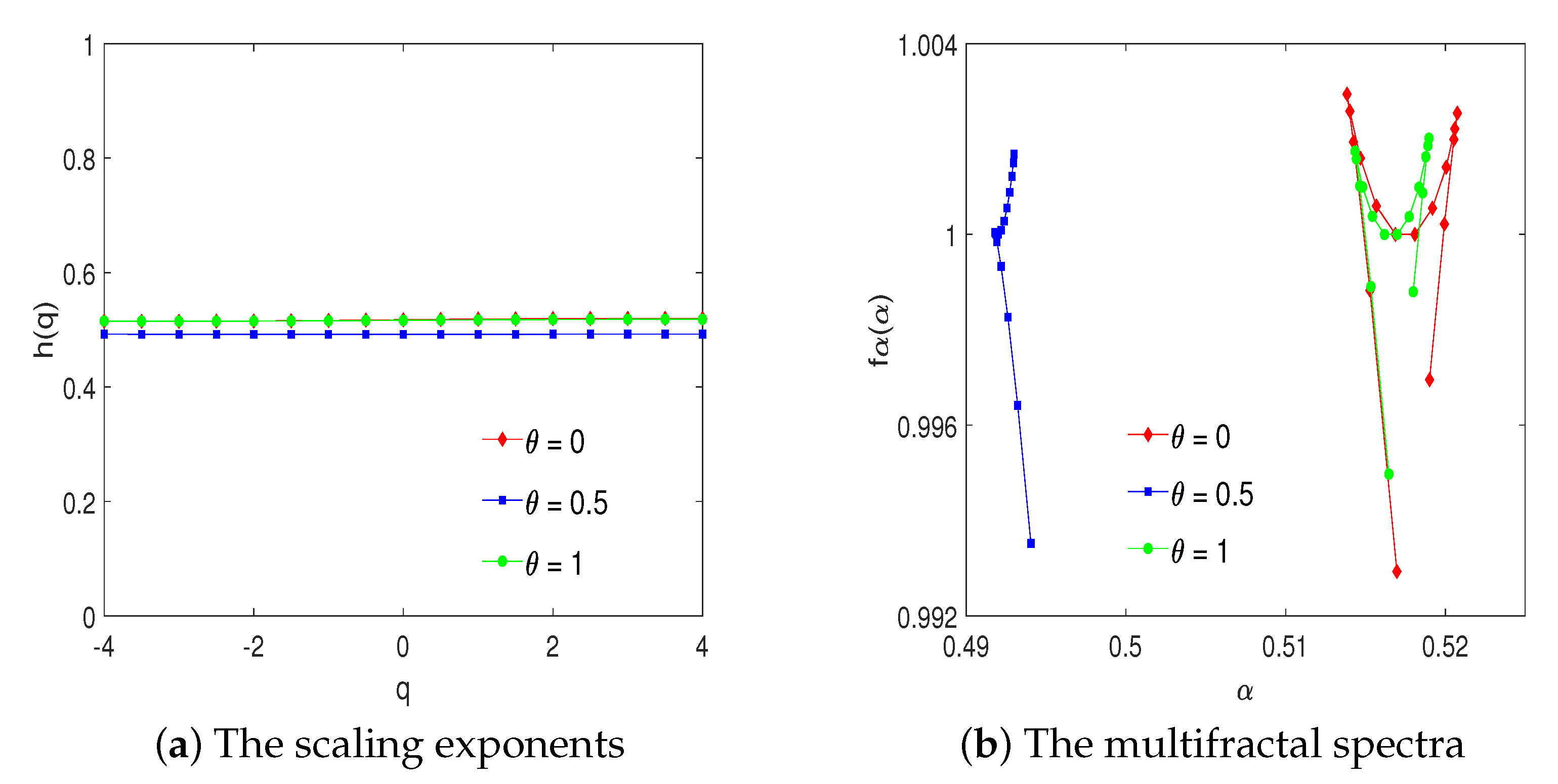
Figure 1 displays the scaling exponents $h\left(q\right)$ as a function of q and multifractal spectra $f\left(\alpha \right)$ obtained by applying the MV-MFDMA to trivariate uncorrelated monofractal series, for $\theta =0,0.5,1$. As expected, regardless of $\theta$, for trivariate uncorrelated monofractal series, the estimated scaling exponent $h\left(q\right)$ equals $0.5$. This result implies the monofractal properties of multivariate series and holds regardless of the parameter $\theta$. The multifractal spectra $f\left(\alpha \right)$ confirms the validity of the algorithm.

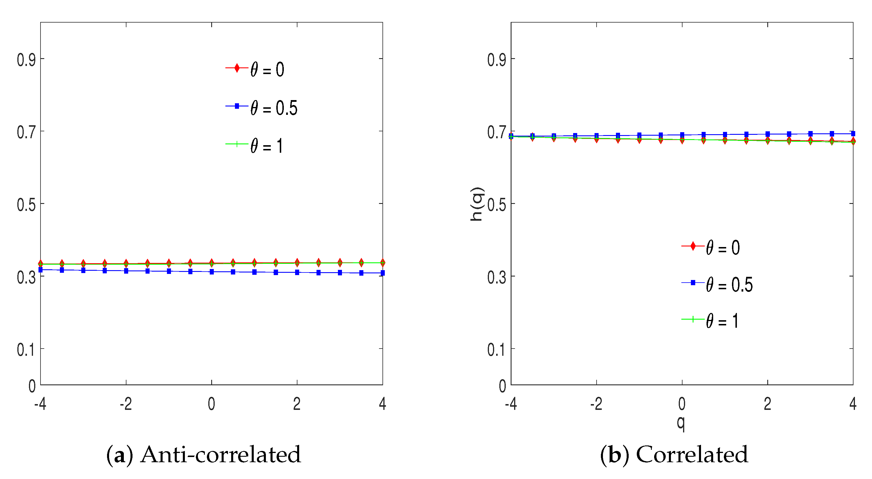
Next, we simulated trivariate anti-correlated and correlated monofractal time series with the following scaling exponents: $h=0.3$$(d=-0.2)$ and $h=0.7$$(d=0.2)$; see Figure 2. The results show that $h\left(q\right)$ is independent of q and practicality equal to $0.3$ and $0.7$, respectively. These results hold regardless of the chosen parameter $\theta$.

3.2. Correlated Bivariate Monofractal Series

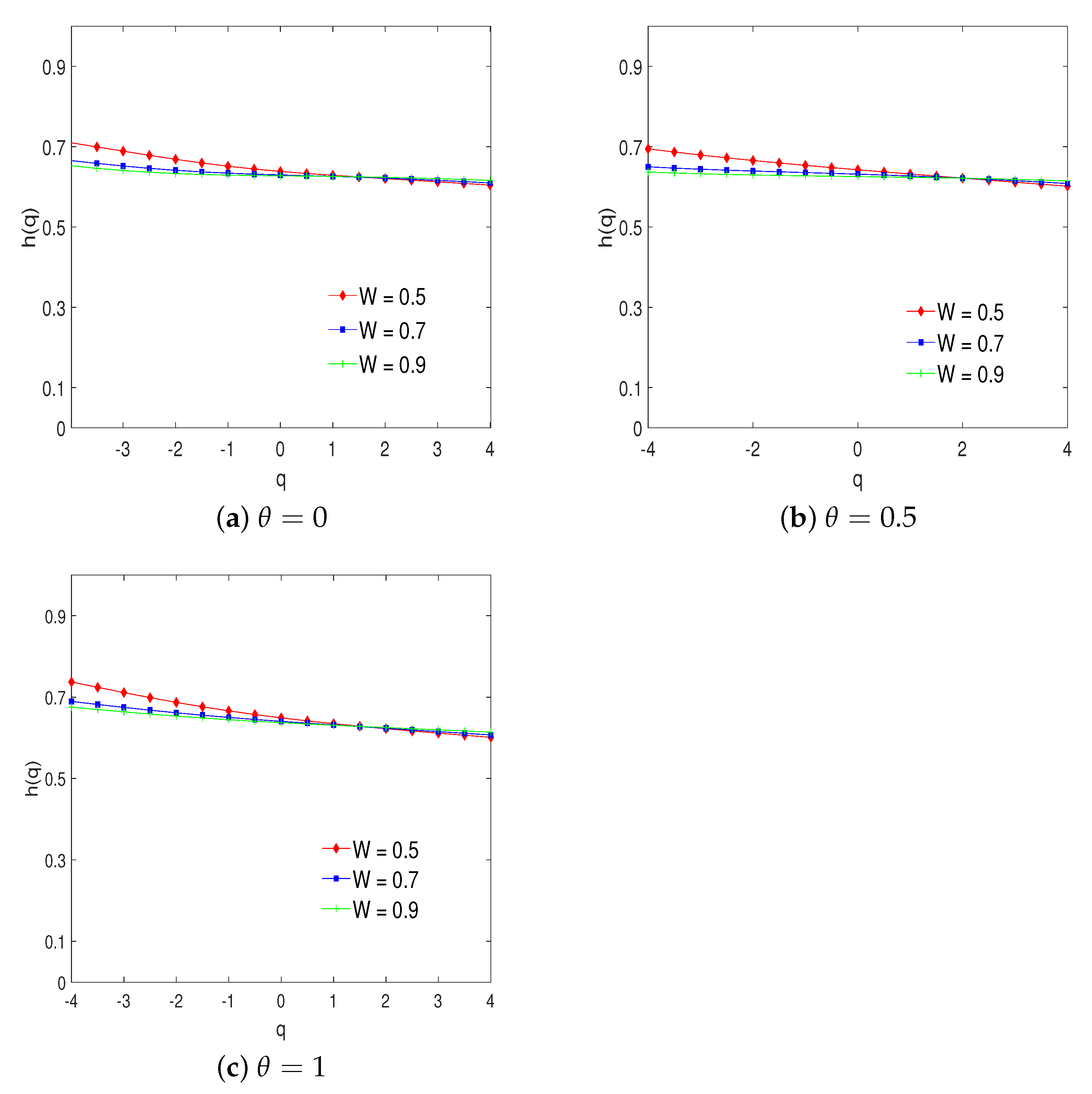
The MV-MFDMA method was also applied and tested on the correlated bivariate time series simulated by the two-component ARFIMA model following the procedure in [12]. The following values of a free parameter controlling the coupling strength between time series were considered: $W=0.5,0.7,0.9$, while the parameters of the model $d_1=d_2=0.2$ corresponded to scaling coefficients $h_1=h_2=0.7$. Figure 3 shows the average MV-MFDMA results of correlated bivariate time series with different correlation levels for $\theta =0,0.5,1$. If we fix the coupling parameter W, the scaling exponents $h\left(q\right)$ do not depend on the value of q and are nearly equal to the value of $0.7$. This result is in harmony with the scaling exponent of individual univariate series. Moreover, even if we change the coupling parameter W, the scaling exponents $h\left(q\right)$ remain the same for different values of q.

3.3. Multivariate Multifractal Series

Finally, we applied the MV-MFDMA to multifractal time series simulated by the following binomial multifractal model:

$$x_k=p_x^{n(k-1)}{(1-p_x)}^{n_{max}-n(k-1)},$$

(11)

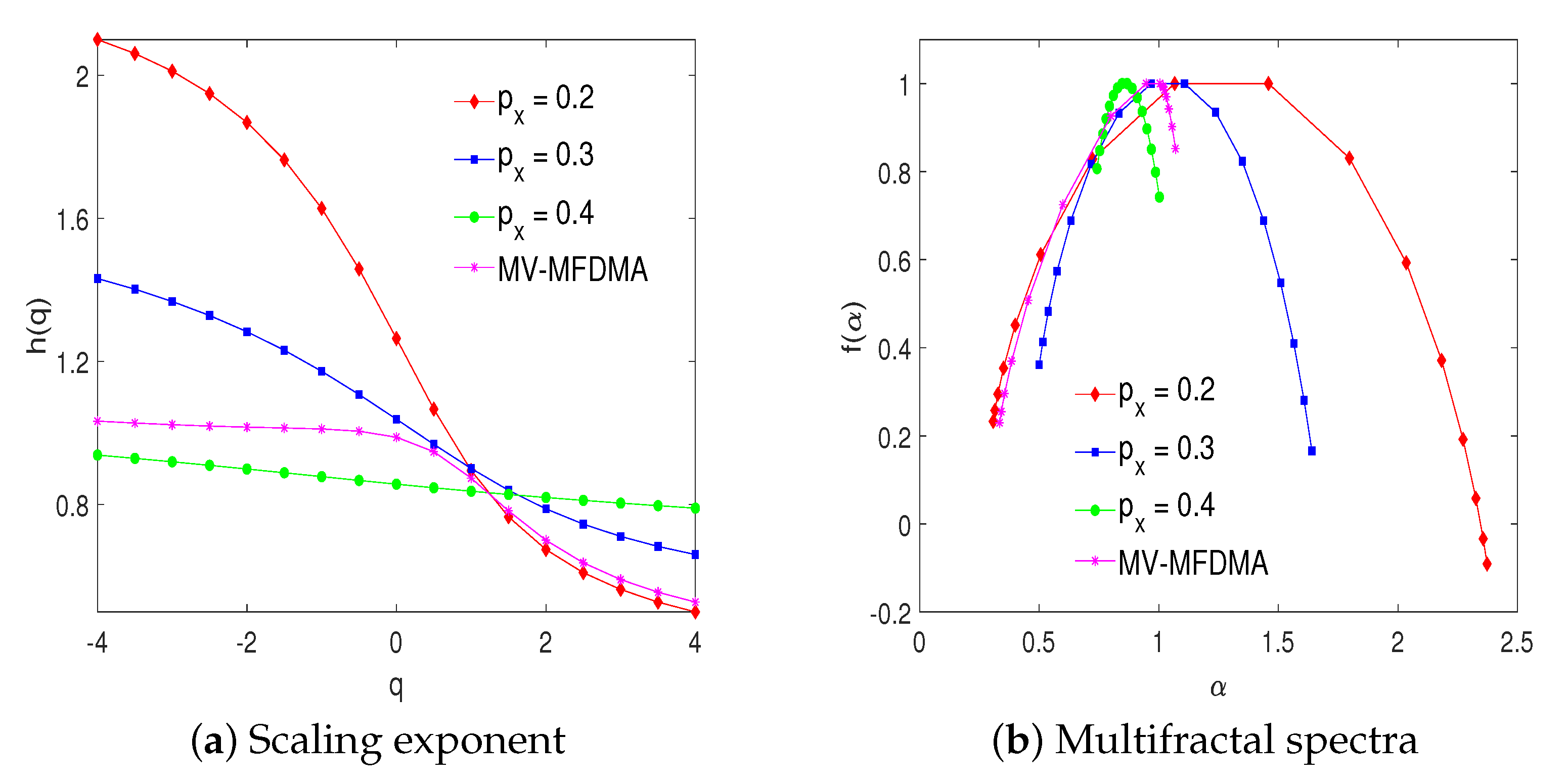
where $p_x\in (0,0.5)$ and $n\left(k\right)$ is the number of the digits equal to one in the binary representation of index k [12]. More precisely, we simulated trivariate time series $x,y,z$ according to (11) and chose $p_x=0.2$, $p_y=0.3$ and $p_z=0.4$, respectively. The proposed algorithm was applied to the generated series, and the obtained results are shown in Figure 4 in terms of scaling exponent $h\left(q\right)$ and multifractal spectra $f\left(\alpha \right)$ for $\theta =0.5$. We also present the same results for individual time series.

The individual univariate time series manifest the expected multifractal characteristics, while it can be observed that the scaling exponents $h\left(q\right)$ of the considered trivariate multifractal series obtained by the new MV-MFDMA vary among the scaling exponents $h\left(q\right)$ of individual univariate series. For negative values of q, the scaling exponents $h\left(q\right)$ of the trivariate multifractal series are most harmonized to the scaling exponents of a univariate series for $p_z=0.4$. On the other hand, for positive values of q, it is most adjusted to the scaling exponents of a univariate series for $p_x=0.2$. This phenomenon was also revealed in [12]. The large fluctuations of univariate series with $p_x=0.2$ have a major impact on the large fluctuation of multivariate series. Similarly, the major impact on the small fluctuations of multivariate series originates from the small fluctuations of univariate series with $p_z=0.4$.

Based on the presented results, we can observe that the MV-MFDMA algorithm preserves the properties of the univariate MFDMA. Namely, it is known that algorithms based on the multifractal detrending moving average are sensitive to the sample size, the selection of the scaling range, the choice of q-orders, and the position of the moving window [23]. These algorithms require a larger sample size, i.e., a larger number of observations are needed to obtain a more accurate estimation of the multifractal spectrum. Then, the accuracy is also influenced by the selection of the appropriate scaling range. Equal spacing between scales is suggested, where the scaling range varies from 10 to $N/10$ [23]. The choice of the q-orders should include both positive and negative values. It is evident from the presented results that the algorithm depends on the position of the moving window. According to [24], the lowest accuracy is obtained when $\theta =0.5$, while $\theta =0$ and $\theta =1$ provide higher accuracy.

A comparison of the proposed MV-MFDMA algorithm with other algorithms for detecting multifractal properties is given in

Table 1. Comparison of the algorithms for detecting multifractality.

Method	Description	Comments
MFDFA [4]	•  applies to univariate time series	•  requires a larger sample size for accurate estimates
	•  detects a long-range correlation and multifractal properties	•  non-overlapping segmentation can cause pseudo fluctuation errors
	•  detrends the original series by removing its average
MFDMA [6]	•  applies to univariate time series	•  requires a larger sample size for accurate estimates
	•  detects a long-range correlation and multifractal properties	•  the backward MFDMA outperforms the MFDFA
	•  detrends the original series by removing the moving average function
MVDFA [1]	•  applies to multivariate time series	•  preserves the characteristics of the univariate DFA
	•  represents a generalization of the DFA	•  characterized by one scaling exponent
	•  describes the autocorrelations’ behavior	•  requires an equal length of time series
MV-MFDFA [12]	•  applies to multivariate time series	•  preserves the characteristics of the univariate MFDFA
	•  represents a generalization of the MFDFA	•  requires an equal length of time series
	•  detects a long-range correlation and the multifractal properties of multichannel data directly
MV-MFDMA Section 2	•  applies to multivariate time series	•  preserves the characteristics of the univariate MFDMA
	•  represents a generalization of the MFDMA	•  requires an equal length of time series
	•  detects a long-range correlation and the multifractal properties of multichannel data directly	•  represents an alternative of both the MV-MFDFA and the MFDMA

.

4. Air Pollutant Time Series via MV-MFDMA

In this section, we present the data and analyze the multifractal properties of multivariate air pollutant time series. We performed the MV-MFDMA algorithm on raw series, seasonally adjusted series, and remainder components and then compared the results.

4.1. Data

Data for this paper were acquired from [25]. For the purposes of testing the MV-MFDMA, we used datasets of five air pollutants presented in

Table 2. Variables.

Variable	Time-Span	Unit	Frequency	State	Monitor Site
Carbon Monoxide (CO)	2010–2019	ppm	daily	California	60010009
Nitrogen Dioxide (NO2)	2010–2019	ppb	daily	California	60010009
Ozone (O3)	2010–2019	ppm	daily	California	60010009
Particulate Matter (PM2.5)	2010–2019	g/m3	daily	California	60010009
Sulfur Dioxide (SO2)	2010–2019	ppb	daily	California	60010011

. To obtain uniform series in terms of length, values were used only on days when all five variables were measured.

Table 3. Descriptive statistics: raw data series.

		CO	NO2	O3	PM2.5	SO2
Mean		0.4375	21.4214	0.0280	8.8429	1.9949
Std. Dev.		0.2508	11.0571	0.0091	7.7520	2.7298
Skewness		1.4251	0.6122	0.1371	8.5209	7.9297
Kurtosis		7.4013	3.4522	4.2429	131.7860	141.7981
Jarque–Bera		3825.237 *	237.0335 *	225.3758 *	2,347,909 *	2,715,223 *
Observations		3339	3339	3339	3339	3339
ADF (AIC)	intercept	−4.4779 *	−4.8280 *	−6.6122 *	−12.1969 *	−7.4589 *
	trend and intercept	−4.5956 *	−5.0117 *	−6.6436 *	−12.1979 *	−8.6055 *
ADF (SIC)	intercept	−5.9964 *	−5.8778 *	−8.0346 *	−16.5856 *	−10.4407 *
	trend and intercept	−6.1243 *	−6.0941 *	−8.0991 *	−16.5850 *	−11.4677 *
PP	intercept	−27.8682 *	−34.4109 *	−40.4884 *	−19.5129 *	−52.3557 *
	trend and intercept	−28.07811 *	−35.2493 *	−40.7289 *	−19.5138 *	−50.2368 *

Note: ADF—augmented Dickey–Fuller unit root test; PP—Philips–Perron unit root test; AIC—Akaike information criterion; SIC—Schwarz information criterion; *—stat.sig. < 0.01

provides the descriptive statistics of the air pollutant time series. Positive values of skewness indicate that the distributions of all air pollutants are positively skewed. Kurtosis is greater than three for all air pollutants, which indicates that the homogeneity of the distribution in all cases is leptokurtic in relation to the normal distribution. The Jarque–Bera test rejects the null hypothesis of normality in air pollutants’ series distribution, which is further corroborated by the fact that kurtosis is larger than three, and there is no zero skewness in any of the five cases. The statistics of the augmented Dickey–Fuller (ADF) unit root test based on both the Akaike (AIC) and Schwarz information criterion (SIC) reject the null hypothesis of a unit root at the 1% significance level. Additionally, the Philips–Perron (PP) test also rejects the null hypothesis of a unit root at the same significance level. Both the ADF and PP tests were done for both the trend and intercept and just the intercept cases. The t-statistics for all six cases of unit root tests are also presented in Table 3 and indicate that the air pollutants series are stationary.

The state of California was chosen because it is usually singled out as a leader in air pollution among other U.S. states. Even though all air pollutants are high in California, the O₃ levels particularly stand out. Since seasonal trends can sometimes influence the multifractal behavior of time series, it is preferable to perform seasonal decomposition; see for example [15,26,27]. It is interesting to note that a common approach for analyzing trendless fluctuations is absent. Nigmatullin and Vorobev [28] stated that in most cases, authors use traditional methods, such as the Fourier method, the wavelet method, Yulmenteyev’s method, and Timashev’s method or some additional processing algorithms that are also based on conventional methods containing some model assumptions and treatment methods associated with continuous mathematics. Nigmatullin, Lino, and Maione [29] pointed out that these sets of methods solve some specific tasks, but cannot be viewed as universal. To address this gap, a universal “platform” for treating various types of different trendless sequences has been proposed (see [28,29] for more details). For the purposes of this paper, we adjusted the considered time series by performing seasonal and trend decomposition using LOESS (STL) decomposition [30]. Through this algorithm, each time series is additively decomposed into deterministic trends, seasonal components, and stochastic remainder components. Removing seasonal components from the raw time series does not significantly influence the descriptive statistics results. All the descriptive statistics and unit root tests conclusions from the raw data are valid for the seasonally adjusted data as well (see Appendix A). 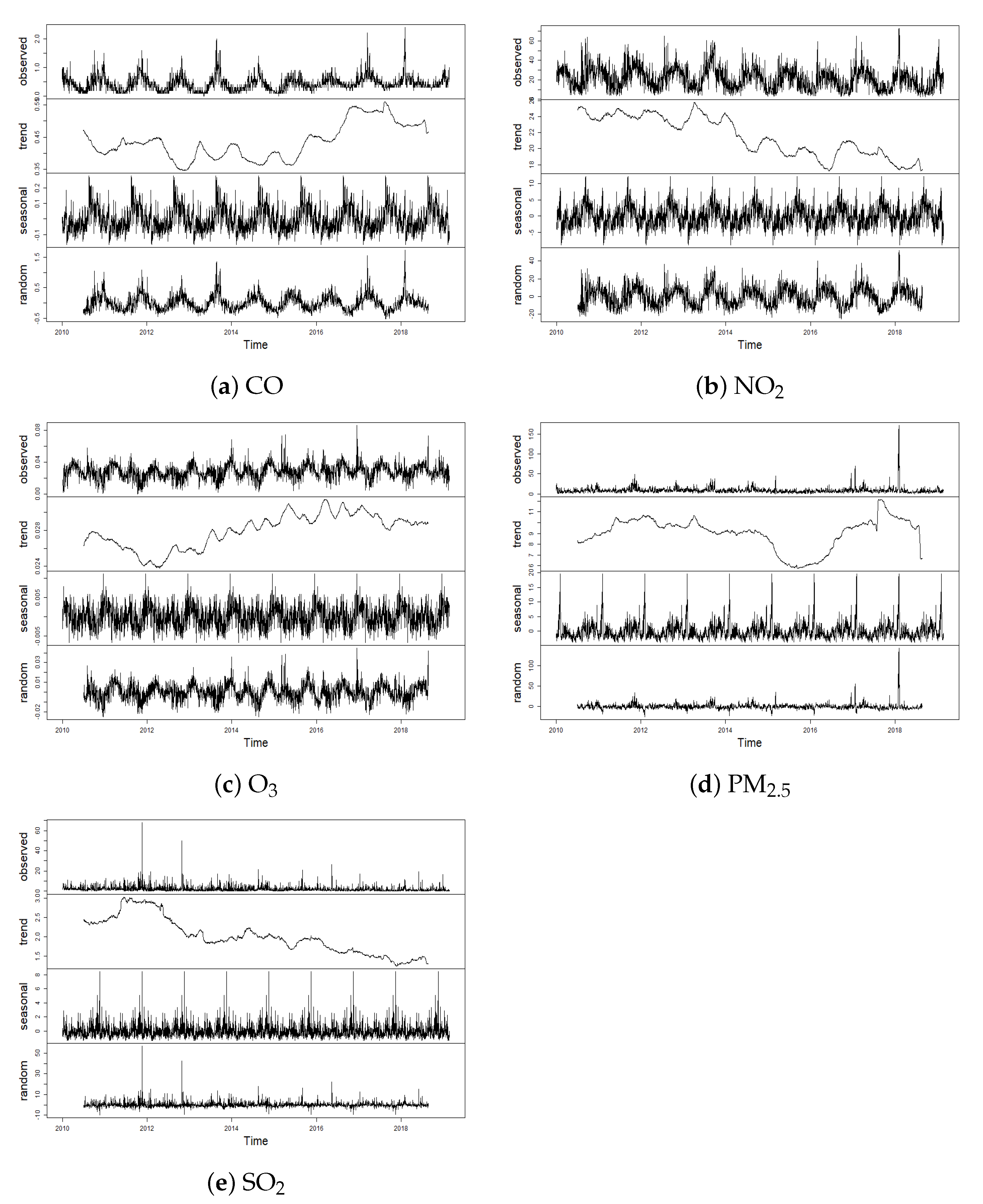Figure 5 shows that the seasonal components of all time series are characterized by the annual oscillation. Figure 5 also demonstrates, among others, the evolution trend of five air pollutant concentration series. The PM_2.5 and SO₂ series are more prone to extreme spikes, whereas NO₂, CO, and O₃ concentrations have somewhat different trends in winter and summer, indicating a seasonal inclination. On the other hand, the trend components are characterized by a very small range of variability and do not show a large temporal evolution. The range of variability is the largest for series NO₂ and PM_2.5. The remainder components of all time series do not display discernible patterns, and there are small fluctuations around zero.

4.2. Results

The MV-MFDMA presented in Section 2 was applied to the above-mentioned raw and seasonally adjusted air pollutant time series obtained upon removal of the seasonal components, as well as on the remainder components of the series. Applying multifractal analysis on the remainder components ensures the identification of the dynamic characteristics of air pollutants’ inner fluctuations and enhances the robustness of the results. We set the range of time scale n to be $10<n<N/10$, where N is the length of each time series.

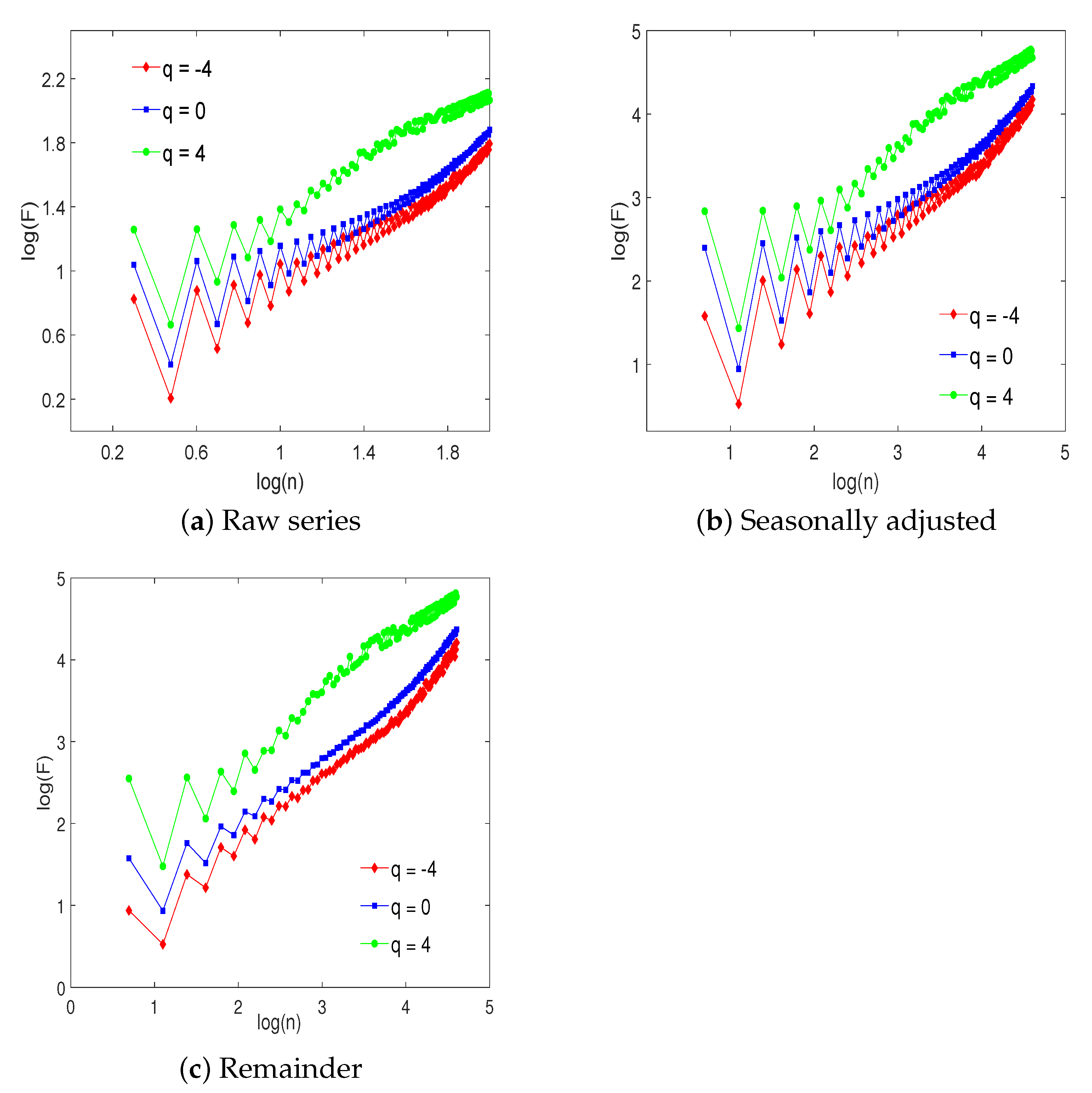
Figure 6 illustrates the behavior of the MV-MFDMA fluctuation function versus time in the logarithmic scale for all three case: raw, seasonally adjusted, and remainder. The plots are presented for $q=-4,0,4$ and fixed $\theta =0.5$. All curves are approximately linear under large scales, indicating the power law behavior and the presence of multifractality. The MV-MFDMA fluctuation functions have quite similar behavior in all three cases, while we can note that fluctuations are the smallest for the remainder components. Fluctuations are observed regardless of the q values for small $log\left(s\right)$ values. That is, the results show crossover time scales, i.e., different scaling laws and scaling exponents for time scales $n<n^{*}$ (where $n^{*}\approx 3.32$ for raw and $n^{*}\approx 12$ for the other two cases). When $n>n^{*}$, we find that the MV-MFDMA fluctuation functions nicely respect the scaling relation, i.e., scale well with the scale size. Additionally, although not displayed, the MV-MFDMA is tested for $\theta =0,1$. The results confirm the power law behavior and demonstrate the absence of large fluctuations.

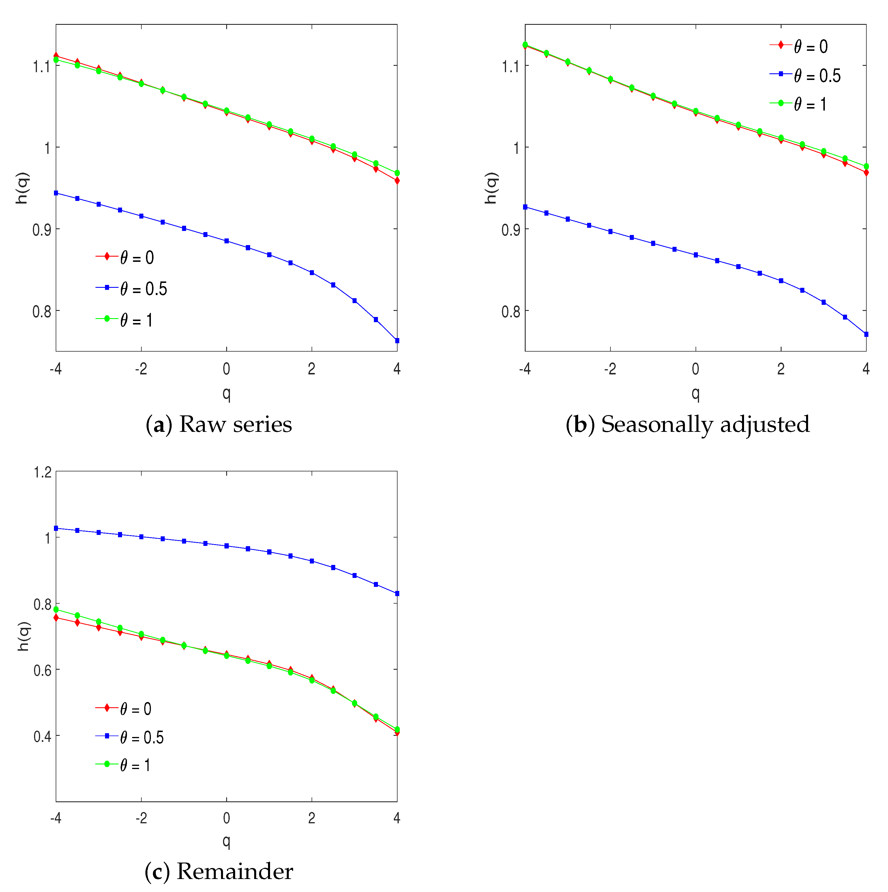
Figure 7 shows the values of the generalized Hurst exponents $h\left(q\right)$ versus q, where the variation of q belongs to the interval $[-4,4]$ for raw, seasonally adjusted, and remainder series. In all cases for $\theta =0,0.5,1$, we observe the dependence of MV-MFDMA $h\left(q\right)$ on q. The MV-MFDMA $h\left(q\right)$ monotonically decreases when the value of q increases. This result implies the multifractality of the examined time series. It is interesting to note that raw and seasonally adjusted series display almost the same behavior of the generalized Hurst exponents $h\left(q\right)$ for all values of parameter $\theta$. On the contrary, the values of the generalized Hurst exponents $h\left(q\right)$ for the remainder series are above $0.5$ for $\theta =0.5$, which indicates a strong long-term persistence. However, in the cases of the forward and backward moving average, the values of $h\left(q\right)$ are lower.

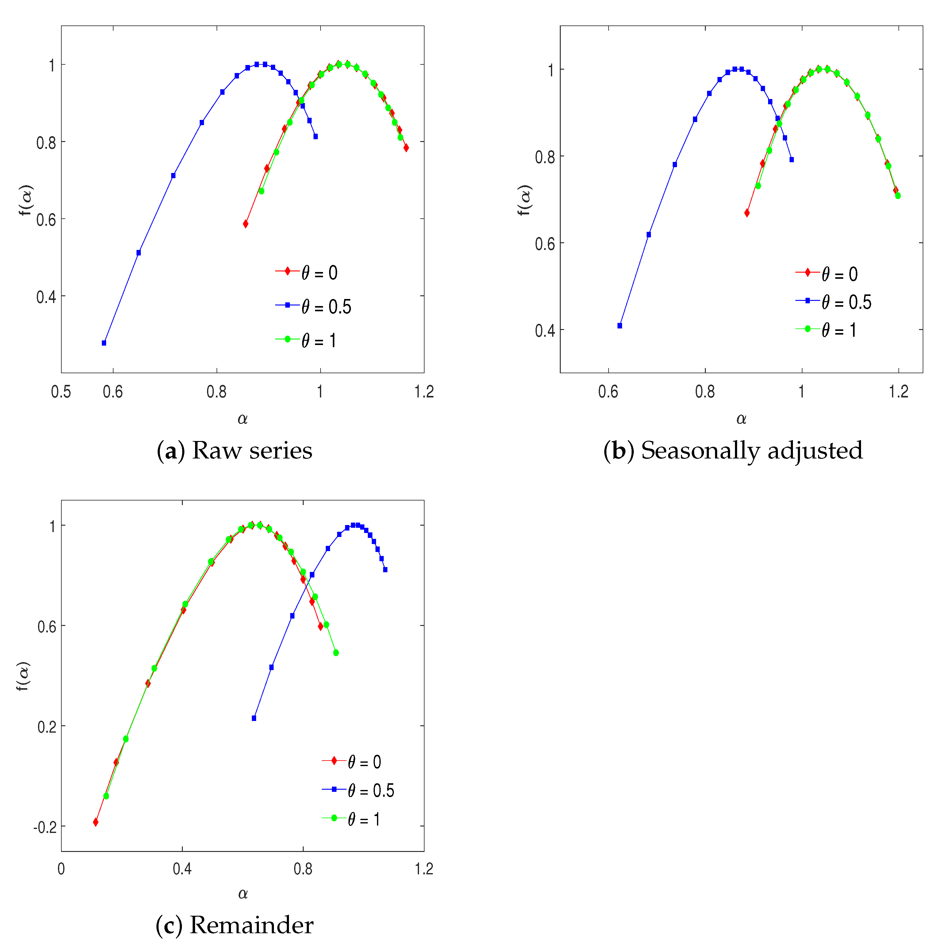
Figure 8 displays the multifractal spectra of $\alpha \sim f\left(\alpha \right)$ via the Legendre transform. The shapes of the inverted U parabola of the spectra confirm the fact of the multifractality in the time series. The smallest range of the multifractality is observed when $\theta =0.5$. The results hold for all raw, seasonally adjusted, and remainder series.

With the aim of quantifying the degree of the multifractality of the multivariate system, we use the following measures (12) and (13) [12]:

$$\mathsf{\Delta }h=maxh\left(q\right)-minh\left(q\right)$$

(12)

$$\mathsf{\Delta }\alpha ={\alpha }_{max}-{\alpha }_{min}.$$

(13)

The larger the measures of $\mathsf{\Delta }h$ and $\mathsf{\Delta }\alpha$, the richer and stronger the degree of multifractality of the time series is.

Table 4. The scaling exponent $h\left(2\right)$, multifractality degrees $\mathsf{\Delta }h$, and $\mathsf{\Delta }\alpha$: raw series.

		CO	NO2	O3	PM2.5	SO2	Multiv.
$\theta =0$	$h\left(2\right)$	0.9980	1.0164	1.0190	0.9823	0.9785	1.0076
$\theta =0.5$		0.9295	0.8741	0.7073	0.7071	0.6414	0.8463
$\theta =1$		0.9937	1.0126	1.0190	0.9775	0.9837	1.0101
$\theta =0$	$\mathsf{\Delta }h$	0.2204	0.1544	0.0559	0.3006	0.2016	0.1525
$\theta =0.5$		0.2074	0.1658	0.0301	0.2875	0.4126	0.1807
$\theta =1$		0.2126	0.1501	0.0559	0.2844	0.3074	0.1387
$\theta =0$	$\mathsf{\Delta }\alpha$	0.3888	0.2678	0.1078	0.6490	0.5710	0.3099
$\theta =0.5$		0.3854	0.3003	0.0650	0.6950	0.7838	0.4080
$\theta =1$		0.3667	0.2573	0.1078	0.6045	0.6098	0.2681

,

Table 5. The scaling exponent $h\left(2\right)$, multifractality degrees $\mathsf{\Delta }h$, and $\mathsf{\Delta }\alpha$: seasonally adjusted series.

		CO	NO2	O3	PM2.5	SO2	Multiv.
$\theta =0$	$h\left(2\right)$	1.1277	1.2088	1.0583	1.0980	1.1991	1.1140
$\theta =0.5$		1.1333	0.9998	0.7086	0.8579	0.7928	0.9192
$\theta =1$		1.1399	1.1881	1.0608	1.1425	1.2301	1.1149
$\theta =0$	$\mathsf{\Delta }h$	0.1758	0.2485	0.0522	0.2778	0.2814	0.1551
$\theta =0.5$		0.2988	0.1793	0.0190	0.3510	0.2923	0.1559
$\theta =1$		0.2002	0.2162	0.0570	0.3208	0.3142	0.1490
$\theta =0$	$\mathsf{\Delta }\alpha$	0.3051	0.4907	0.1006	0.6269	0.5462	0.3076
$\theta =0.5$		0.6336	0.3357	0.0385	0.8267	0.5706	0.3557
$\theta =1$		0.3834	0.4052	0.1150	0.7193	0.6135	0.2891

and

Table 6. The scaling exponent $h\left(2\right)$, multifractality degrees $\mathsf{\Delta }h$, and $\mathsf{\Delta }\alpha$: remainder component.

		CO	NO2	O3	PM2.5	SO2	Multiv.
$\theta =0$	$h\left(2\right)$	0.6209	0.6123	0.5481	0.3940	0.4522	0.5727
$\theta =0.5$		1.0275	0.9819	0.8858	0.7224	0.6188	0.9279
$\theta =1$		0.6206	0.6065	0.5603	0.3878	0.4435	0.5669
$\theta =0$	$\mathsf{\Delta }h$	0.4764	0.3253	0.3109	0.6585	0.5222	0.3471
$\theta =0.5$		0.1945	0.1448	0.1793	0.4061	0.3391	0.1974
$\theta =1$		0.4954	0.3624	0.3160	0.6304	0.3737	0.3632
$\theta =0$	$\mathsf{\Delta }\alpha$	0.8184	0.6024	0.5106	1.1022	1.0444	0.7440
$\theta =0.5$		0.3740	0.2705	0.3500	0.7443	0.6627	0.4341
$\theta =1$		0.8240	0.6388	0.5368	1.0571	0.7054	0.7603

present the scaling exponent $h\left(2\right)$ and the multifractality degrees $\mathsf{\Delta }h$ and $\mathsf{\Delta }\alpha$ for the individual and multivariate air pollutants for all levels $\theta =0,0.5,1$ and for raw, seasonally adjusted, and remainder series, respectively.

Raw and seasonally adjusted series have similar characteristics of multifractal parameters. For $\theta =0$ and $\theta =1$, the values of $h\left(2\right)$ are approximately around one, while in the case of $\theta =0.5$, the values are a bit lower, namely $h\left(2\right)\approx 0.85$ and $h\left(2\right)\approx 0.9$ for raw and seasonally adjusted series, respectively. This holds for both individual and multivariate time series. The results imply that both individual and multivariate series show persistent long-range correlation. Analogous to $1/f$, noise can be deducted in the case of the scaling exponent $h\left(2\right)$ of multivariate time series less than one. In the case of the remainder components, the fluctuations are also characterized by a long-term persistence. However, the values of $h\left(2\right)$ suggest that the remainder components are characterized by a weak persistence suggesting stable trends in the next period. In summary, multivariate series of five air pollutants show consistent, positive autocorrelation behavior. In all three cases, an interesting fact is that all values of $\mathsf{\Delta }h$ and $\mathsf{\Delta }\alpha$ are significantly larger than zero. On the other hand, the values for multivariate air pollutants range around those values for individual time series and are lower than the maximum values of the individuals in each case. Both the $\mathsf{\Delta }h$ and $\mathsf{\Delta }\alpha$ values in the remainder components are higher than the values of both raw and seasonally adjusted series. This finding reveals that the considered air pollutants can be characterized by multifractality behavior. Furthermore, since the relationship always exists among the individuals, it possibly makes the multifractal level weaker. As a result, the $\mathsf{\Delta }h$ and $\mathsf{\Delta }\alpha$ values for multivariate time series are smaller than the maximum and average of the $\mathsf{\Delta }h$ and $\mathsf{\Delta }\alpha$ values of individuals.

5. Conclusions

The multivariate approach and analysis may have a key role in cases when a high degree of uncertainty and coupling underlying dynamical mechanics is present. Hence, in this paper, we introduced the multivariate multifractal detrended moving average analysis (MV-MFDMA) as a multivariate generalization of the MFDMA method. The proposed method provides a way to analyze and investigate fractal dynamics information in multivariate time series data sets generated by complex systems. The validity of the proposed method was investigated by conducting numerical simulations on synthetic monofractal and multifractal time series. The correlation properties of multivariate monofractal time series are in line with the univariate case, and the fractal behavior of correlated bivariate time series is independent of its correlation level. In the case of the multivariate multifractal series, the multivariate system exhibits multifractal properties. The corresponding multifractal degree decreases with the decreasing of the multifractal degree of individual series. According to our simulation results, the MV-MFDMA represents a reliable technique for measuring the long-term correlations of non-stationary multivariate time series.

The MV-MFDMA was also utilized to investigate the multifractal properties of air pollutant time series where the individual air pollutants were considered as different variables from the same system. We analyzed raw and seasonally adjusted time series of air pollutants obtained upon removing the annual oscillations. We found that air pollutants exhibited multifractal auto-correlation behavior, even after removing the seasonal pattern. In both cases, the air pollutant time series data exhibited multifractal properties, with persistent long-range correlations. In order to capture the dynamic characteristics of the inner fluctuations of the air pollutants, we also applied the algorithm to the stochastic remainder components of the time series. The results confirmed that multivariate time series of air pollutants possessed multifractal properties and exhibited long-term persistence such that an increase (decrease) in the previous period will be followed by an increase (decrease) in the next period.

The findings of this paper provide an elevated understanding of the evolutionary activity and temporal links of five air pollutants in the state of California. In general, it is necessary to achieve a better comprehension of the associations between different air pollution time series to manage the environmental air quality based on evidence. Researchers from any scientific field that operate with multivariate frequent time series are encouraged to apply the proposed algorithm since it provides an improvement in detecting long-range correlations and multifractal properties of multichannel data. However, the proposed algorithm has certain limitations. It applies only to frequent and large-dimensional multivariate time series with an equal length N. Moreover, when applying the proposed algorithm, it is suggested to use an equal spacing between scales, where the scaling range varies from 10 to $N/10$, while the q-orders should include both positive and negative values. Finally, in some cases, seasonality can influence the selected time series, so if that is the case, the series should be firstly depersonalized before applying the algorithm. Future research papers can use the proposed MV-MFDMA algorithm, not only the environmental quality ones, but on the widest range of different real-world complex system time series, for example on financial, economic, meteorological, and health care time series. Therefore, directions for future research should go towards studying new time series when a better comprehension of their interconnections is necessary.