Article

Empowering Advanced Driver-Assistance Systems from Topological Data Analysis

1
PIMM Lab, Arts et Metiers Institute of Technology, 151 boulevard de l’Hopital, 75013 Paris, France
2
Departamento de Matemáticas, Física y Ciencias Tecnológicas, Universidad Cardenal Herrera-CEU, CEU Universities, San Bartolome 55, 46115 Alfara del Patriarca, Valencia, Spain
3
I3A, Aragon Institute of Engineering Research, Universidad de Zaragoza, 50018 Zaragoza, Aragon, Spain
4
Department of Mechanical and System Design Engineering, Hongik University, 94 Wausanro, Mapogu, Seoul 04066, Korea
5
Digital Human Lab, Hongik University, 94 Wausanro, Mapogu, Seoul 04066, Korea
6
ESI Group, 3bis rue Saarinen, CEDEX 1, 94528 Rungis, France
*
Author to whom correspondence should be addressed.
Mathematics 2021, 9(6), 634; https://doi.org/10.3390/math9060634
Submission received: 31 January 2021 / Revised: 6 March 2021 / Accepted: 11 March 2021 / Published: 16 March 2021
(This article belongs to the Special Issue Numerical Simulation in Biomechanics and Biomedical Engineering)

Abstract

:
We are interested in evaluating the state of drivers to determine whether they are attentive to the road or not by using motion sensor data collected from car driving experiments. That is, our goal is to design a predictive model that can estimate the state of drivers given the data collected from motion sensors. For that purpose, we leverage recent developments in topological data analysis (TDA) to analyze and transform the data coming from sensor time series and build a machine learning model based on the topological features extracted with the TDA. We provide some experiments showing that our model proves to be accurate in the identification of the state of the user, predicting whether they are relaxed or tense.

1. Introduction

While there have recently been considerable advances in self-driving car technology, driving still relies mainly on human factors. Even in self-driving mode, human drivers must often make decision in a fraction of a second to avoid accidents. Therefore, it is still of utmost importance to develop systems capable of discerning if the human driver is attentive or not to the road conditions. In general, the so-called advanced driver assistance systems (ADAS) [1,2] are systems that are able to improve the driver’s performance, among which, adaptive speed limiters, pedestrian detectors [3], and cruise controllers are some of the most popular systems. Fatigue alerting systems are among the most useful among ADAS systems, and the aim of this work is to contribute to the development of such a system based on a systematic analysis of drivers in actual driving conditions.
The estimation of the driver’s condition (degree of attention to the road, fatigue, etc.) is a very important factor to ensure safety in driving [4,5]. A recent review on the topic can be found in [6]. The goal of this work is to extract behavior patterns from car user data to be able to accurately estimate their state. We used data obtained by the laboratory of prof. Hyung Yun Choi at Hongik University in Seoul. His experiment involved the application of mechanical stimulation to people seated in an automobile.
Our main goal is to extract patterns of behavior from experimental data so as to allow us to learn the most relevant factors affecting driver’s attention to the situation of the road.
In the present work, we combine some tools from Morse theory [7] and topological data analysis (TDA) with all of the associated concepts and methods (e.g., Betti numbers, homology persistence, barcodes, persistence images, etc.) [8], most of them introduced and employed later in order to analyze and classify the experimental data. This allows us to introduce concepts as barcodes, that is, persistent and life-time diagrams in a similar way to how they are used in persistent homology. Our main goal is to predict car user behavior following a supervised approach [9]. Instead of considering an original sensor signal as the quantity of interest, we focus on its topological features. In this sense, the framework proposed in this paper allows us to unveil the true dimensionality of data or, in other words, the actual number of factors affecting driver’s performance. Thus, we model a sensor signal as a dynamical system, and, therefore, our approach seems to be better at describing its properties, or rather its variations, such as extrema, patterns, and self-similarity, than other approaches. We note that our approach is, in some senses, similar to that followed by Milnor and Thurston [10] in the study of the combinatorial properties of dynamical systems by combining tools from automata theory.
The structure of the paper is as follows: In Section 2, we describe the material and methods employed in this work. Particular attention is paid to the process of data acquisition and the description of time series and data curation. In Section 3, we present the main results of this work, and we discuss the main consequences in Section 4. As a complement, in Appendix A, we thoroughly illustrate the process of computing persistence images for the data of interest.

2. Material and Methods

In this section, we describe the collection and preprocessing of the experimental data. In Section 2.1, we describe the data acquisition, and in Section 2.2, we provide a description of the time series. Section 2.3 is devoted to data preprocessing. The mathematical tools used to describe the times series at a topological level are explained in Section 2.4. Finally, the image classification methodology is given in Section 2.5.

2.1. Data Acquisition

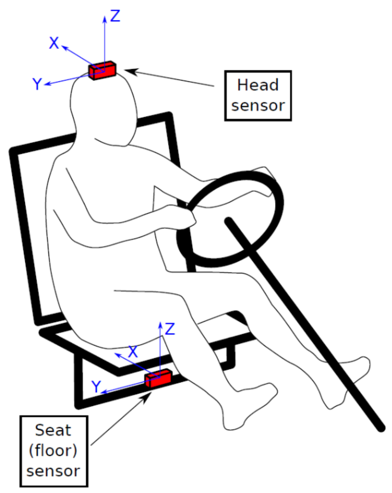
Our proposed predictor directly uses the data collected from the experiments. The data acquisition process involves measuring the response of human behavior when an excitation is applied to the seat. Figure 1 shows the location of the sensors in the experiments.
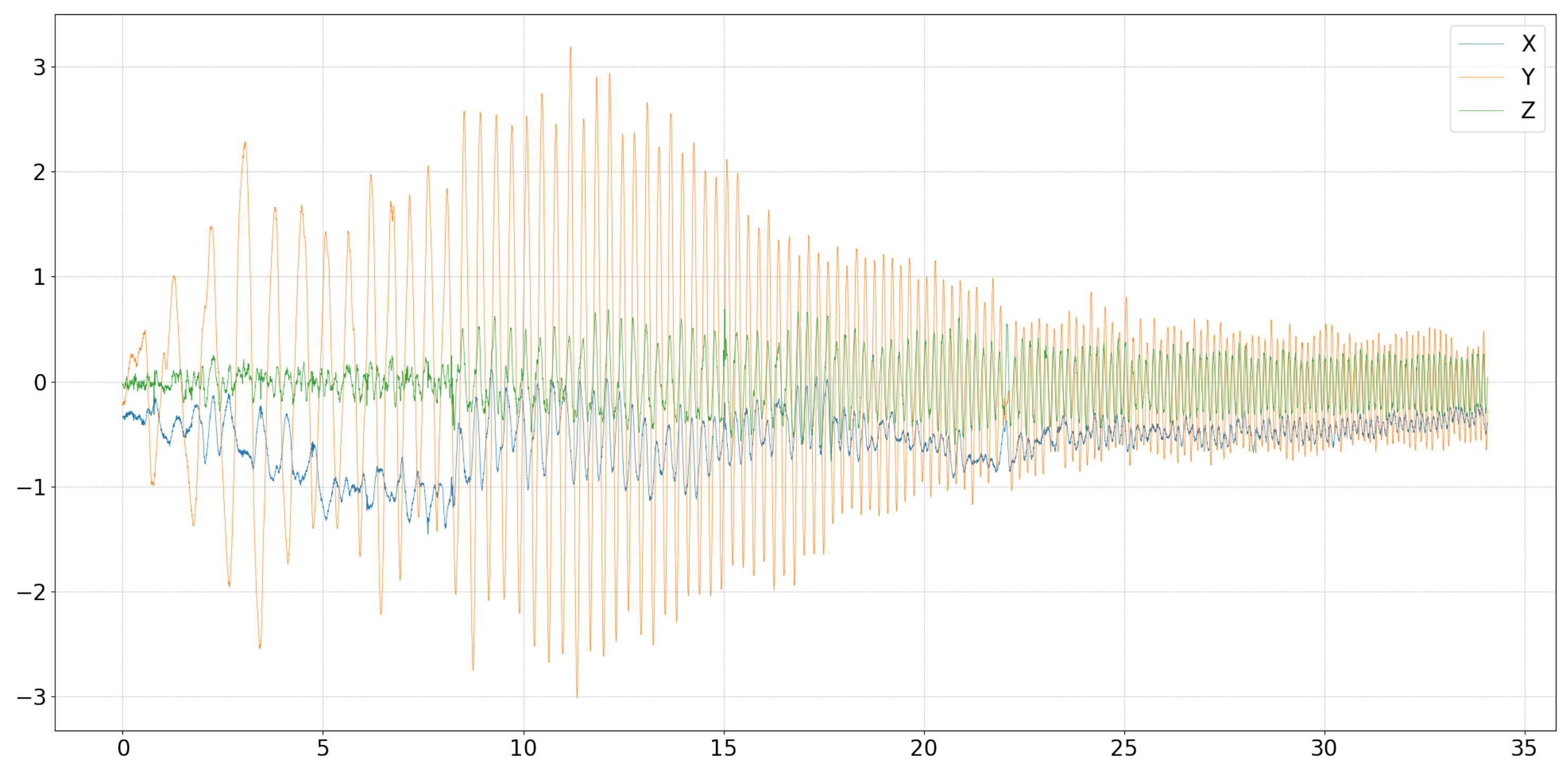
The excitation signal is an angular acceleration imposed on the seat of the user. This acceleration is an oscillating chirp function with a frequency range of 1 to 7.5 Hz on the X axis in rotation. The linear acceleration a = ( a x , a y , a z ) and angular velocity ω = ( ω x , ω y , ω z ) were measured in both the head and the seat by two IMU (Shimmer inertia measurement unit (IMU) sensors) at 256 Hz. By observing the floor excitation signals, we noted that the excitation is purely rotational around the X-axis—see Figure 2.
Several experiences were conducted by nine people by taking into account a set of six fixed states: driver, passenger, tense person, relaxed person, rigid seat, and SAV (sport activity vehicle seat). In particular, for each individual, eight experiments for the six available states were performed:
Class Label 1 SAVRelaxedPassager 2 SAVTensePassager 3 SAVRelaxedDriver 4 SAVTenseDriver 5 RigidRelaxedPassager 6 RigidTensePassager 7 RigidRelaxedDriver 8 RigidTenseDriver
As a consequence, we worked with a sample of 72 experiences, each of them encoded in a time series (as we explain later). Our goal is to classify the behavior of a generic driver, assigning one of the two states (tense or relaxed) by using the sensor data.

2.2. Time Series Description

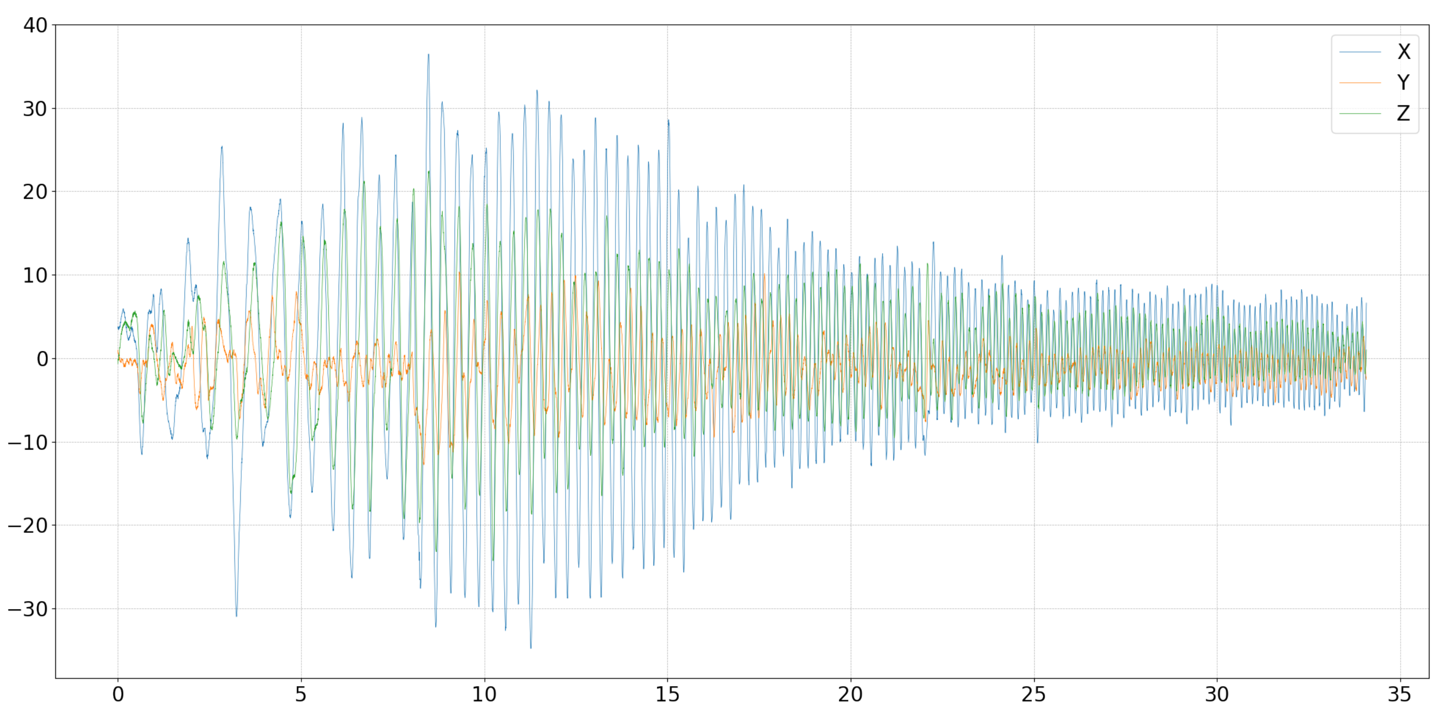
The data acquired from sensors (see Figure 3 and Figure 4) were stored into six-dimensional time series, for both linear acceleration and angular velocity of the head movement. The sampling frequency of the data was 256 Hz, and the duration of the experiment was 34 s; hence, the resulting data dimensionality is 256 × 34 = 8704 . For each times series, where 1 t 8704 , we constructed three new times series called the sliding window, embedding a length of 5800. The first one is given by the times values from t = 1 to t = 5800 , the second is given by the times values from t = 1450 to t = 7250 , and, to conclude, the third time window is defined as from t = 2904 to t = 8704 . Each element in the sample ( 1 i 72 ) was encoded by means of three six-dimensional time series representing each of the three sliding windows that we represent in matrix form as follows:
T S 3 ( i 1 ) + 1 = a x ( 1 ) a x ( 2 ) a x ( 5800 ) a y ( 1 ) a y ( 2 ) a y ( 5800 ) a z ( 1 ) a z ( 2 ) a z ( 5800 ) ω x ( 1 ) ω x ( 2 ) ω x ( 5800 ) ω y ( 1 ) ω y ( 2 ) ω y ( 5800 ) ω z ( 1 ) ω z ( 2 ) ω z ( 5800 ) , T S 3 ( i 1 ) + 2 = a x ( 1450 ) a x ( 1451 ) a x ( 7251 ) a y ( 1450 ) a y ( 1451 ) a y ( 7251 ) a z ( 1450 ) a z ( 1451 ) a z ( 7251 ) ω x ( 1450 ) ω x ( 1451 ) ω x ( 7251 ) ω y ( 1450 ) ω y ( 1451 ) ω y ( 7251 ) ω z ( 1450 ) ω z ( 1451 ) ω z ( 7251 )
and
T S 3 i = a x ( 2903 ) a x ( 2905 ) a x ( 8704 ) a y ( 2903 ) a y ( 2905 ) a y ( 8704 ) a z ( 2903 ) a z ( 2905 ) a z ( 8704 ) ω x ( 2903 ) ω x ( 2905 ) ω x ( 8704 ) ω y ( 2903 ) ω y ( 2905 ) ω y ( 8704 ) ω z ( 2903 ) ω z ( 2905 ) ω z ( 8704 ) .
Here, the matrices have a size of 6 × 5800 and 1 i 72 . This allows us to represent the information by using a third-order tensor, namely, Z R 216 × 6 × 5800 defined by
Z i , j , k : = ( T S i ) j , k
for 1 i 216 , 1 j 6 and 1 k 5800 . We can identify Z i = T S i for 1 i 216 .

2.3. Data Preprocessing

In order to obtain a single series for each observation, we concatenated all of the 6 time series (linear accelerations and angular velocities) for each observation horizontally and then created a data frame by stacking the 216 in sample observations.
The concatenation operation on the multidimensional time series collapsed the last two dimensions into one dimensional arrays with a length of 5800 × 6 = 34,800 . The result is the two-dimensional table of concatenated time series
D = v e c ( Z 1 , : , : ) v e c ( Z 216 , : , : ) R 216 × 34800 .
We chose not to filter the signals because the topological sub-level set method should filter the high-frequency features naturally. We also chose to keep working on acceleration signals in order to avoid signal deviations after two integrations in time so as to obtain positions, the sensors not always keeping a zero mean height. Thus, the approach is completely (topologically) data-based.
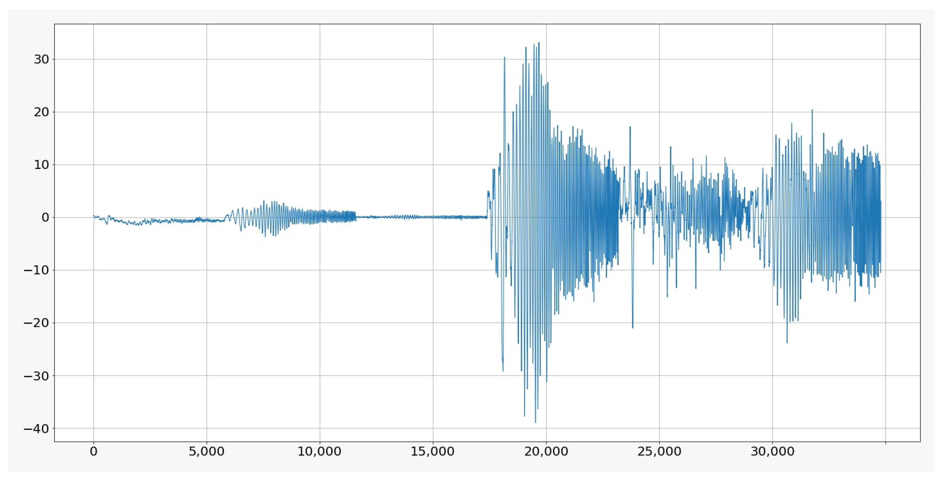
The six time series Z i of each observation were collapsed into a single concatenated time series with a size of 34,800—see Figure 5. The concatenated time series for the 216 observations were then stacked to create the dataset D with a size of 216 × 34,800. We also used binary labels in the chained time series Z i on the two target classes that we were interested in. In particular, we wrote Z i ( α ) where α is "0" for a relaxed driver and “1” for a tense one.

2.4. Extracting Topological Features from a Time Series

The idea to extract the topological information regarding the times series is to consider each sample observation as a piecewise linear continuous map from a closed interval to the real line. Therefore, we used a construction closely related to the Reeb graph [11] used in Morse theory to describe the times series at the topological level.
To this end, we consider the time series x t for 0 t N 1 ( N 3 ) given by a vector
X = ( x 0 , x 1 , , x N 1 ) R N .
we can view X as a function also denoted by X : { 0 , 1 , , N 1 } R defined by X ( i ) = x i for 0 i N 1 . Here, to study the topological features of X we use the sub-level set of a piecewise-linear function f X : R R associated with X satisfying that f X ( i ) = X ( i ) = x i for 0 i N 1 .
To construct this function, we consider the basis functions { φ 0 , , φ N 1 } of continuous functions φ i : R R defined by
φ i ( s ) : = s i + 1 if i 1 s i i + 1 s if i s i + 1 0 if s ] i 1 , i + 1 [
where i = 1 , , N 2 and
φ 0 ( s ) : = 1 s if 0 s 1 0 if s [ 0 , 1 ]
φ N 1 ( s ) : = s N + 2 if N 2 s N 1 0 if s [ N 2 , N 1 [
This allows us to construct a piecewise continuous map f X : R R by
f X ( s ) = j = 0 N 1 x j φ j ( s ) ,
and also to endow R N with a norm given by
X : = f X L 2 ( R ) = | f X ( s ) | 2 d s 1 / 2 .
In particular, we prove the following result, which helps us to identify the time series given by the vector X in R N with the function f X in L 2 ( R ) .
Proposition 1.
The linear map Φ : ( R N , · ) ( L 2 ( R ) , · L 2 ( R ) ) given by Φ ( X ) = f X is an injective isometry between Hilbert spaces. Furthermore, Φ ( R N ) is a closed subspace in L 2 ( R N ) .
Proof. 
The map is clearly isometric and injective because { φ 0 , , φ N 1 } is a set of linear independent functions in L 2 ( R ) . □
Here, we describe the maps f X Φ ( R N ) at the combinatorial level using the connected components (intervals) associated with its λ sub-level sets
LS λ ( f X ) : = { x [ 0 , N 1 ] : f X ( x ) λ }
for λ R . For this purpose, we introduce the following distinguished objects related to the supp ( f X ) = [ 0 , N 1 ] R of f X :
  • The nodes or vertices denoted by
    V : = { [ 0 ] , [ 1 ] , , [ N 1 ] }
    that represent the components of the vector X , ;
  • The faces denoted by
    F : = { [ 0 , 1 ] [ 1 , 2 ] , , [ N 2 , N 1 ] }
    that represent the intervals used to construct the connected components of the sub-level sets of the map f X . Recall that we consider
    [ i , i + 1 ] : = { z R : z = μ x i + 1 + ( 1 μ ) x i , 0 μ 1 } R .
Let
λ max = max s [ 0 , N 1 ] f X ( s ) = max 0 i N 1 X ( i ) ,
and
λ min = min s [ 0 , N 1 ] f X ( s ) = min 0 i N 1 X ( i ) .
For each λ min λ λ max , we introduce the following symbolic λ sub-level set for the map f X :
L S λ ( f X ) : = σ F : f ( σ ) λ
For λ min λ λ λ max , it holds
L S λ ( f X ) L S λ ( f X ) .
Our next goal was to quantify the evolution of the above symbolic λ sub-level with. To this end, we introduce the notion of feature associated with the λ sub-level set L S λ ( f X ) .
We define the set of features for functions in Φ ( R N ) as
F ( Φ ( R N ) ) : = [ i , j ] R : 0 i < j N 1 .
We note that L S λ ( f X ) F F ( Φ ( R N ) ) . Then next definition introduces the notion of features for a symbolic λ sub-level set as the interval of F ( Φ ( R N ) ) constructed by a maximal union of faces of L S λ ( f X ) .
Definition 1.
We suggest that I F ( Φ ( R N ) ) is a feature for the symbolic λ sub-level set L S λ ( f X ) if there exists I 1 , , I k L S λ ( f X ) such that I = j = 1 k I k and for every J L S λ ( f X ) such that J I i for 1 i k it holds that I J = . We denote by F ( L S λ ( f X ) ) the set of features for the λ sub-level set L S λ ( f X ) .
A feature for a λ sub-level set L S λ ( f X ) is the maximal interval of F ( Φ ( R N ) ) that we can construct by unions of intervals in L S λ ( f X ) . To illustrate this definition, we give the following example:
Example 1.
Let us consider the time series
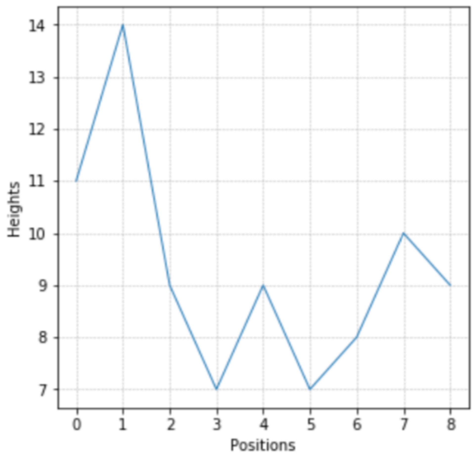
X = ( 11 , 14 , 9 , 7 , 9 , 7 , 8 , 10 , 9 ) .
This allows us to construct the map f X as shown in Figure 6. Then, λ m i n = 7 and λ max = 14 , and we have the following symbolic λ sub-level sets.
L S λ = 7 ( f X ) = L S λ = 8 ( f X ) = L S λ = 7 ( f X ) { [ 5 , 6 ] } L S λ = 9 ( f X ) = L S λ = 8 ( f X ) { [ 2 , 3 ] , [ 3 , 4 ] , [ 4 , 5 ] } L S λ = 10 ( f X ) = L S λ = 9 ( f X ) { [ 6 , 7 ] , [ 7 , 8 ] } L S λ = 11 ( f X ) = L S λ = 10 ( f X ) L S λ = 12 ( f X ) = L S λ = 11 ( f X ) L S λ = 13 ( f X ) = L S λ = 11 ( f X ) L S λ = 14 ( f X ) = L S λ = 11 ( f X ) { [ 0 , 1 ] } .
This allows us to compute the available features for each λ-value:
λ = 7 λ = 8 λ = 9 λ = 10 λ = 11 λ = 12 λ = 13 λ = 14
F ( L S λ ( f X ) ) [ 5 , 6 ] [ 2 , 6 ] [ 2 , 8 ] [ 2 , 8 ] [ 2 , 8 ] [ 2 , 8 ] [ 0 , 8 ]
Let F ( f X ) be the whole set of features for f X , that is,
F ( f X ) = I : I F ( L S λ ( f X ) ) for some λ min λ λ max .
Example 2.
From Example 1, we obtain
F ( f X ) = { [ 5 , 6 ] , [ 2 , 6 ] , [ 2 , 8 ] , [ 0 , 8 ] } .
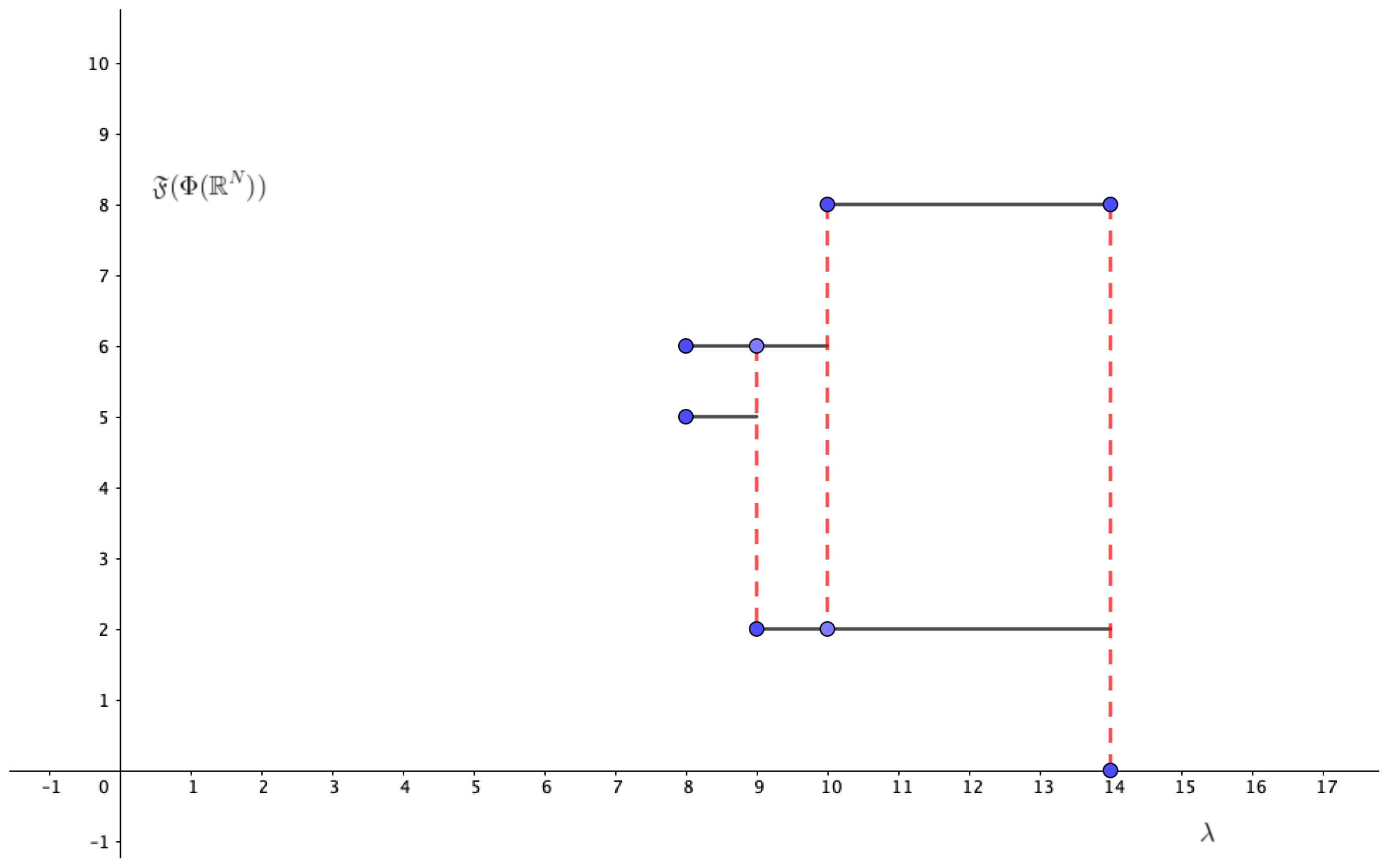
We can represent the map λ L S λ ( f X ) from [ λ min , λ max ] to F ( f X ) as shown in Figure 7.
Let I F ( f X ) ; in order to quantify the persistence of this particular feature for the map f X , we use the map λ L S λ ( f X ) from [ λ min , λ max ] to F ( f X ) . To this end, we introduce the following definition: the birth point of the feature I is defined by
a ( I ) = inf λ : I F ( L S λ ( f X ) )
and the corresponding death point by
b ( I ) = sup λ : I F ( L S λ ( f X ) ) .
In particular, we note that a ( [ 0 , N 1 ] ) = λ max (see Figure 7). Since a ( I ) b ( I ) < holds for all I F ( f X ) , I [ 0 , N 1 ] , we call the finite interval [ a ( I ) , b ( I ) ] the barcode of the feature I F ( f X ) \ { [ 0 , N 1 ] } .
Example 3.
From Example 1 we consider the features [ 5 , 6 ] L S λ = 8 ( f X ) , [ 2 , 6 ] L S λ = 9 ( f X ) , and [ 2 , 8 ] L S λ = 10 ( f X ) . Then, the feature [ 5 , 6 ] has its birth point at a ( [ 5 , 6 ] ) = 8 and its death point at b ( [ 5 , 6 ] ) = 9 ; the feature [ 2 , 6 ] has its birth point at a ( [ 2 , 6 ] ) = 9 and its death point at b ( [ 2 , 6 ] ) = 10 . Finally, the feature [ 2 , 8 ] has its birth point at a ( [ 2 , 8 ] ) = 10 and its death point at b ( [ 2 , 8 ] ) = 14 . As a consequence, the set
B ( f X ) : = { ( [ 5 , 6 ] ; 8 , 9 ) , ( [ 2 , 6 ] ; 9 , 10 ) , ( [ 2 , 8 ] ; 10 , 14 ) }
of features and its corresponding barcodes contain the relevant information of the shape of f X (see Figure 7).
Thus, we define the set of barcodes for f X by
B ( f X ) = ( I ; a ( I ) , b ( I ) ) : I F ( f X ) \ { [ 0 , N 1 ] }
and its persistence diagram as
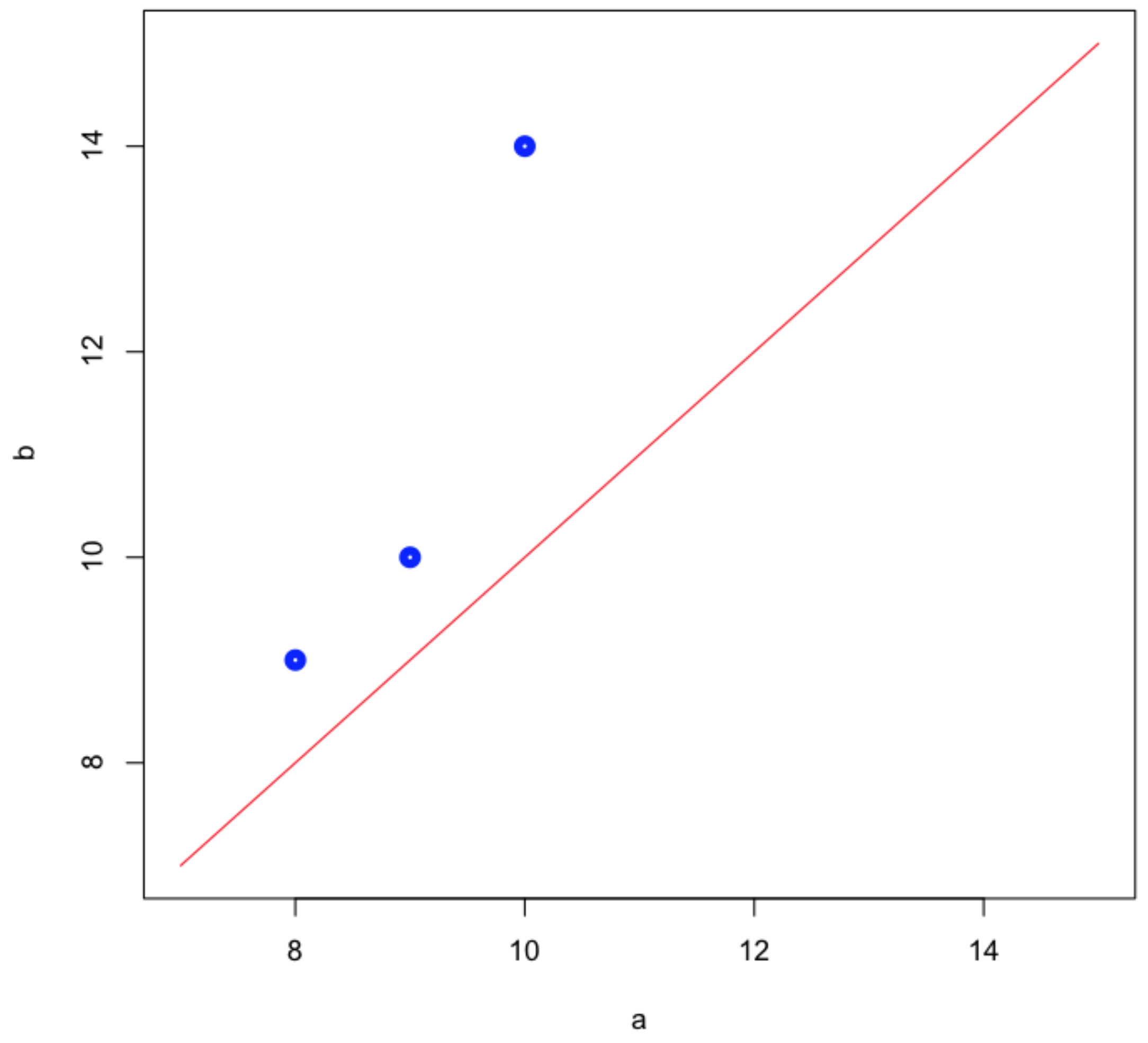
PD ( f X ) : = ( a ( I ) , b ( I ) ) R 2 : I F ( f X ) \ { [ 0 , N 1 ] }
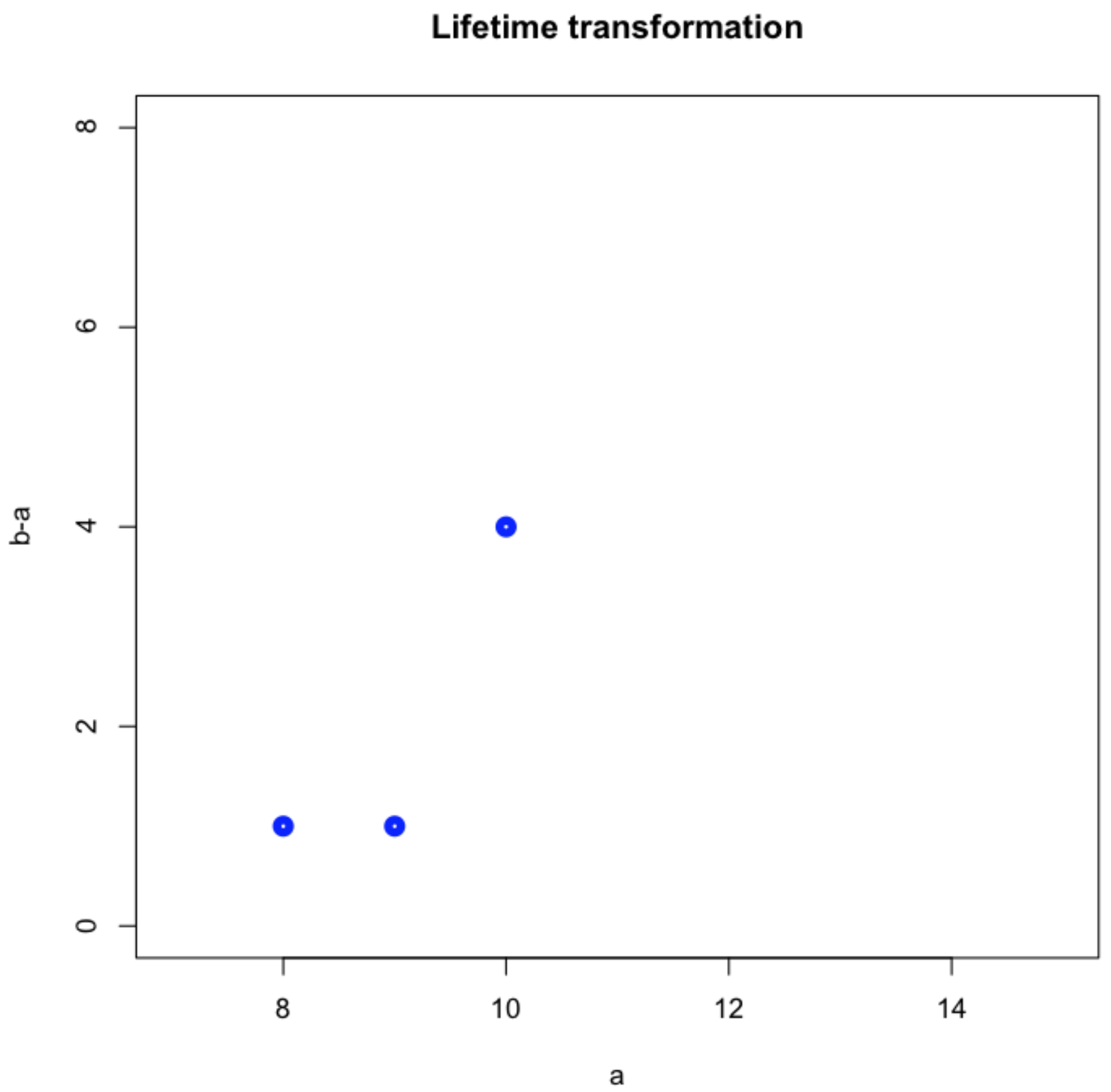
(see Figure 8). An equivalent representation of the persistence diagram is the life-time diagram for f X , which is constructed by means of a bijective transformation T ( a , b ) = ( a , b a ) , acting over PD ( f X ) , that is,
LT ( f X ) : = ( a ( I ) , b ( I ) a ( I ) ) R 2 : I F ( f X ) ) \ { [ 0 , N 1 ] } ;
see Figure 9.
In order to determine the grade of similarity between two barcodes from two different time series, we need to set a similarity metric. To this end, we construct the persistent image for f X as follows: we observe that LT ( f X ) is a finite set of points, namely,
LT ( f X ) = { ( a 1 , b 1 a 1 ) , , ( a k , b k a k ) }
for some natural numbers k 1 and such that b 1 a 1 b 2 a 2 b k a k . Then, we consider a non-negative weighting function w : LT ( f X ) [ 0 , 1 ] given by
w ( a i , b i a i ) = b i a i b k a k for 1 i k
.
Finally, we fix M, a natural number, and take a bivariate normal distribution g u ( x , y ) centered at each point u LT ( f X ) and with its variance σ i d = 1 M max 1 i k ( b i a i ) i d , where i d is the 2 × 2 identity matrix. A persistence kernel is then defined by means of a function ρ X : R 2 R , where
ρ X ( x , y ) = u LT ( f X ) w ( u ) g u ( x , y ) .
We associate with each X R a matrix in R M × M as follows: let ε > 0 be a non-negative real number that is sufficiently small, and then consider a square region Ω X , ε = [ α , β ] × [ α * , β * ] R 2 , covering the support of ρ X ( x , y ) (up to a certain precision), such that
Ω X , ε ρ X ( x , y ) d x d y 1 ε
holds. Next, we consider two equispaced partitions of the intervals
α = p 0 p 1 p M = β and α * = p 0 * p 1 * p M * = β * .
Now, we put
Ω X , ε = i = 0 M 1 j = 0 M 1 [ p i , p i + 1 ] × [ p j * , p j + 1 * ] = i = 0 M 1 j = 0 M 1 P i , j
The persistence image of X associated with the partition P = { P i , j } is then described by the matrix given by the following equation:
P I ( X , M , P , ε ) = P i , j ρ X ( x , y ) d x d y i = 0 , j = 0 i = M 1 , j = M 1 R M × M .

2.5. Classification

Image classification is a procedure that is used to automatically categorize images into classes by assigning to each image a label representative of its class. A supervised classification algorithm requires a training sample for each class, that is, a collection of data points whose class of interest is known. Labels are assigned to each class of interest. The classification problem applied to a new observation is thus based on how close a new point is to each training sample. The Euclidean distance is the most common distance metric used in low-dimensional datasets. The training samples are representative of the known classes of interest to the analyst. In order to classify the persistence diagrams, we can use any state-of-the-art technique. In our case, we considered the random forest classification.
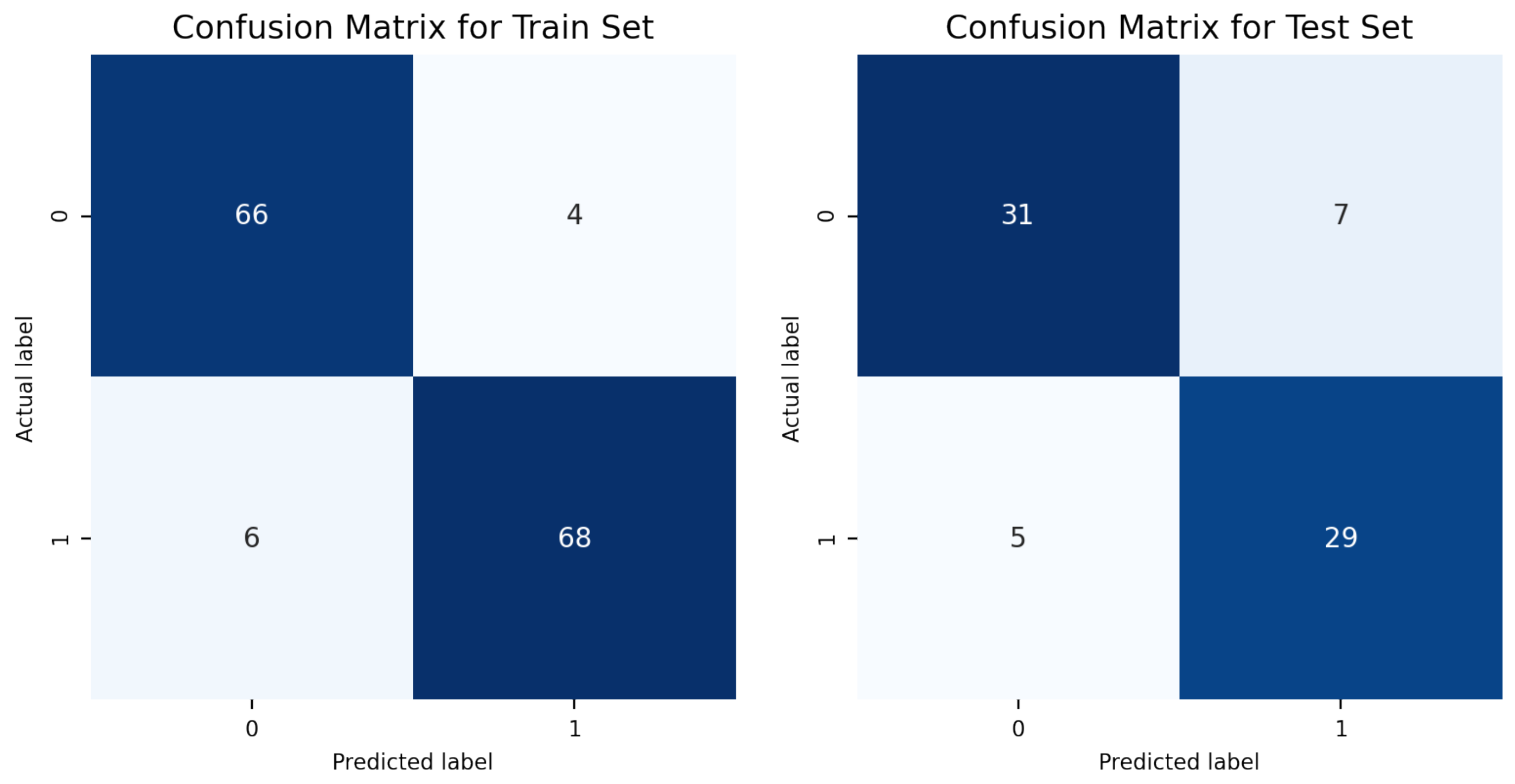
Recall that we conducted 9 different experiments, with 24 samples associated with each one of them corresponding to 3 samples for each of the different experimental conditions: relaxed rigid driver, relaxed rigid passenger, relaxed SAV driver, relaxed SAV passenger, tense rigid driver, tense rigid passenger, tense SAV driver, and tense SAV passenger. Their respective labels are { 0 , 0 , 0 , 0 , 1 , 1 , 1 , 1 } . Therefore, we designed the following training validation process: The model is trained over 144 samples and evaluated over the remaining unseen 72 experiments (two-to-one training-to-testing ratio). The split between training and sampling is achieved using random shuffling and stratification to ensure balance between the classes. In order to improve the evaluation of the model generalizability, we also performed a cross-validation procedure following a leave-one-out strategy, consisting of iteratively training over the full dataset except one sample that was left out and used to test and score the model. We used the accuracy metric to evaluate the classification model. We can represent the performance of the model using the so-called confusion matrix: a 2D entries table where elements account for the number of samples in each category, with the first axis representing the true labels and the second axis the predicted labels. We also computed the different classification metrics to obtain a more detailed reporting of the model performances.

3. Results

The trained random forest classifier model for the persistence images has a notably high accuracy score on the training dataset (144) for both approaches and high accuracy for the testing dataset (72 samples). This suggests strong differentiation of the images with the respect to their generating signals, see Figure 10. The scores on the training and testing are 93 and 83%, respectively. The leave-one-out cross-validation achieved a score of 81%, indicating a good variance–bias trade-off and good generalization potential of the model.

4. Discussion

The combination of Morse theory and topological data analysis allows us to extract information from real data without the need for smoothness or regularity assumption on the time series. In our case, input data for each experiment were reduced from six-sensor time series of measurements to one single image containing the persistent pattern for attention to the road. Using the obtained persistence images as the new inputs, supervised learning proved to successfully predict the attention state of the driver or passenger.
The procedure used and described in this paper does not involve any additional pre-processing of the sensor data; is robust to noise and degraded signals; and supports large quantities of data, which makes it efficient and scalable.
It is important to highlight the fact that while the proposed methodology based on the TDA (successfully applied in large datasets [9]) seems general and powerful and it was able to extract the main data features, the validity of the driver behaviors observed in the analyzed dataset should be carefully checked due to the overly reduced dataset employed (limited to nine individuals) that does not allow for the full validation of prediction robustness.

Author Contributions

Conceptualization, F.C., H.Y.C. and M.H.; data curation, T.F., A.B. and M.H.; formal analysis, F.C., A.F., A.B., E.C., H.Y.C. and J.-L.D.; funding acquisition, F.C.; investigation, T.F., A.F. and M.H.; methodology, F.C., A.F., A.B. and H.Y.C.; software, A.B.; supervision, F.C., E.C. and H.Y.C.; writing—original draft, T.F.; writing—review editing, A.B. and E.C. All authors have read and agreed to the published version of the manuscript.

Funding

This research was funded by ESI Group, Contract 2019-0060 with the University of Zaragoza.

Institutional Review Board Statement

Ethical review and approval were waived for this study due to the research presents no risk of harm to subjects and only collects non-personalized anonymized data.

Informed Consent Statement

Informed consent was obtained from all subjects involved in the study.

Data Availability Statement

Data are available under request.

Conflicts of Interest

The authors declare no conflict of interest. The funders had no role in the design of the study; in the collection, analyses, or interpretation of data; in the writing of the manuscript, or in the decision to publish the results.

Appendix A

We can illustrate the process of computing the persistence diagrams, the lifetime diagrams, and the persistence images for the driver time series for each experimental setup:
  • Relaxed driver with SAV seat;
  • Relaxed driver with rigid seat;
  • Relaxed passenger with SAV seat;
  • Relaxed passenger with rigid seat;
  • Tense driver with SAV seat;
  • Tense driver with rigid seat;
  • Tense passenger with SAV seat;
  • Tense passenger with rigid seat.
Figure A1. Relaxed driver with SAV seat.
Mathematics 09 00634 g0a1
Figure A2. Relaxed driver with rigid seat.
Mathematics 09 00634 g0a2
Figure A3. Relaxed passenger with SAV seat.
Mathematics 09 00634 g0a3
Figure A4. Relaxed passenger with rigid seat.
Mathematics 09 00634 g0a4
Figure A5. Tense driver with SAV seat.
Mathematics 09 00634 g0a5
Figure A6. Tense driver with rigid seat.
Mathematics 09 00634 g0a6
Figure A7. Tense passenger with SAV seat.
Mathematics 09 00634 g0a7
Figure A8. Tense passenger with rigid seat.
Mathematics 09 00634 g0a8

Appendix B

To better evaluate a classification model, we are interested in quantities that express how often a sample is correctly or wrongly labelled into a particular class over all the samples and all the classes:
  • A T r u e p o s i t i v e (TP): the correct prediction of a sample into a class;
  • A T r u e n e g a t i v e (TN): the correct prediction of a sample out of a class;
  • A F a l s e p o s i t i v e (FP): the incorrect prediction of a sample into a class;
  • A F a l s e n e g a t i v e (FN): the incorrect prediction of a sample out of class.
Therefore, we can examine in more detail the classification model performance using the following metrics:
  • The p r e c i s i o n P is the number of correct positive results divided by the number of all positive results.
    P = T P T P + F P
  • The r e c a l l R is the number of correct positive results divided by the number of all relevant samples.
    R = T P T P + F N
  • The F-1 score is the harmonic mean of precision and recall.
    F 1 = 2 × P × R P + R
  • The a c c u r a c y A is the number of correct predictions over the number of all samples.
    A = T P + T N T P + T N + F P + F N
We can summarize the presented metrics for our model in the following two reports:
Figure A9. Classification report.
Mathematics 09 00634 g0a9

References

  1. Paul, A.; Chauhan, R.; Srivastava, R.; Baruah, M. Advanced Driver Assistance Systems (No. 2016-28-0223); SAE Technical Paper; SAE International: Warrendale, PA, USA, 2016. [Google Scholar] [CrossRef]
  2. Shaout, A.; Colella, D.; Awad, S.S. Advanced Driver Assistance Systems-Past, Present and Future. In Proceedings of the 2011 Seventh International Computer Engineering Conference (ICENCO’2011), Cairo, Egypt, 27–28 December 2011; pp. 72–82. [Google Scholar]
  3. Geronimo, D.; Lopez, A.M.; Sappa, A.D.; Graf, T. Survey of pedestrian detection for advanced driver assistance systems. IEEE Trans. Pattern Anal. Mach. Intell. 2009, 32, 1239–1258. [Google Scholar] [CrossRef] [Green Version]
  4. Lindgren, A.; Chen, F. State of the art analysis: An overview of advanced driver assistance systems (adas) and possible human factors issues. Hum. Factors Econ. Asp. Saf. 2006, 38, 50. [Google Scholar]
  5. Izquierdo-Reyes, J.; Ramirez-Mendoza, R.A.; Bustamante-Bello, M.R. A study of the effects of advanced driver assistance systems alerts on driver performance. Int. J. Interact. Des. Manuf. 2018, 12, 263–272. [Google Scholar] [CrossRef]
  6. Sikander, G.; Anwar, S. Driver fatigue detection systems: A review. IEEE Trans. Intell. Transp. Syst. 2018, 20, 2339–2352. [Google Scholar] [CrossRef]
  7. Milnor, J. Morse Theory; Princeton University Press: Princeton, NJ, USA, 1963. [Google Scholar]
  8. Epstein, C.; Carlsson, G.; Edelsbrunner, H. Topological data analysis. Inverse Probl. 2011, 27, 120201. [Google Scholar]
  9. Frahi, T.; Argerich, C.; Youn, M.; Chinesta, F.; Falco, A. Tape surfaces characterization with persistence images. AIMS Mater. Sci. 2020, 7, 364–380. [Google Scholar] [CrossRef]
  10. Milnor, J.W.; Thurston, W. On iterated maps of the interval, Dynamical systems (College Park, MD, 1986–87). In Lecture Notes in Mathematics; Springer: Berlin/Heidelberg, Germany, 1988; pp. 465–563. [Google Scholar]
  11. Reeb, G. Sur les points singuliers d’une forme de Pfaff complètement intégrable ou d’une fonction numérique. C. R. Acad. Sci. Paris 1946, 222, 847–849. [Google Scholar]
Figure 1. Scheme of the data acquisition process showing the location of the sensors.
Mathematics 09 00634 g001
Figure 2. Floor excitation: X-axis angular velocity time series.
Mathematics 09 00634 g002
Figure 3. Sensor data: linear acceleration time series.
Mathematics 09 00634 g003
Figure 4. Sensor data: angular velocity time series.
Mathematics 09 00634 g004
Figure 5. Tensor reduction of a sensor time series.
Mathematics 09 00634 g005
Figure 6. The map f X for X = ( 11 , 14 , 9 , 7 , 9 , 7 , 8 , 10 , 9 ) .
Mathematics 09 00634 g006
Figure 7. The map λ L S λ ( f X ) for X = ( 11 , 14 , 9 , 7 , 9 , 7 , 8 , 10 , 9 ) .
Mathematics 09 00634 g007
Figure 8. Persistence diagram for the map f X when X = ( 11 , 14 , 9 , 7 , 9 , 7 , 8 , 10 , 9 ) .
Mathematics 09 00634 g008
Figure 9. Life-time diagram for the map f X when X = ( 11 , 14 , 9 , 7 , 9 , 7 , 8 , 10 , 9 ) .
Mathematics 09 00634 g009
Figure 10. Model performance for prediciting the attention state.
Mathematics 09 00634 g010
Publisher’s Note: MDPI stays neutral with regard to jurisdictional claims in published maps and institutional affiliations.