Regression Models in Complex Survey Sampling for Sensitive Quantitative Variables

Abstract

Randomized response (RR) techniques are widely used in research involving sensitive variables, such as drugs, violence or crime, especially when a population mean or prevalence must be estimated. However, they are not generally applied to examine relationships between a sensitive variable and other characteristics. This type of technique was initially applied to qualitative variables, and studies later showed that a logistic regression may be performed with RR data. Since many of the variables considered in this context are quantitative, RR techniques were extended to these cases to estimate the values required. Regression analysis is a valuable statistical tool for exploring relationships among variables and for establishing associations between responses and covariates. In this article, we propose a design-based regression analysis for complex sample designs based on the unified RR approach. We present estimators of the regression coefficients, study their theoretical properties and consider different ways to estimate their variance. The properties of these estimation techniques were simulated using various quantitative randomized models. The method proposed was also used to analyse the findings from a real-world survey.

1. Introduction

Standard randomized response (RR) methods are mainly used in surveys that elicit a binary response to a sensitive question in order to estimate the proportion of the study population presenting a given (sensitive) characteristic. Warner’s study generated a rapidly expanding body of research literature on alternative techniques for eliciting suitable RR schemes in order to estimate such a population proportion ([1,2,3,4,5,6]).

Some studies addressed situations in which the response to a sensitive question results in a quantitative variable and when the researcher wishes to estimate a linear parameter as the mean or the total of the sensitive variable under study. In the method proposed by [7], the interviewee was asked to choose, by means of a randomization device, from two questions; one concerned the sensitive variable and the other was unrelated (both were of the same order of magnitude). Other important papers in this regard include [8,9,10,11,12,13,14,15,16,17,18,19,20,21], together with the contributions compiled by [22,23,24,25,26]. When dealing with quantitative sensitive variables, the idea is that respondents should not disclose the true value of the sensitive variable but rather provide a scrambled value, which is obtained by algebraically perturbing the true response. This is done by applying one or more scrambling random variables, independent from each other and from the sensitive variable, the distributions of which are fully known to the researcher.

RR methods were also been applied to examine relationships between a qualitative sensitive variable and other variables. Thus, reference [27] showed that logistic regression may be performed with RR data, and [28] developed multivariate regression logistic techniques for four RR designs. In addition, reference [29] considered the univariate logistic regression model for binary RR response variables and presented this model as a generalized linear model. The same research group also developed a multivariate logistic regression model for RR response variables. Under simple random sampling, reference [30] considered a generalized linear model and generalized linear mixed models for RR designs where the probability of obtaining a positive response can be written as a linear equation of the answer to the sensitive question. Finally, reference [31] presented a logistic regression model on RR data when the covariates for some subjects were randomly missing.

However, few prior studies were made of regression techniques for quantitative randomized response variables. reference [32] performed a linear regression analysis using the model presented in [10] for the simple random sampling case, from which the variance of the estimate was calculated. In a related paper, reference [33] discussed the maximum likelihood estimation of an independently and identically distributed normal linear regression model when some of the covariates are subject to RR.

In this paper, we address the question of regression techniques for quantitative RR data under a general sampling design. Specifically, we consider a general class of RR methods ([34]) for quantitative variables and show how the RR can be used as the outcome in regression models.

The rest of this paper is organized as follows. First, we review the unified RRT approach described by [21] to establish the framework, and clarify the notation used (Section 2). We then show how RR can be used as the outcome in regression models, present estimators for the regression coefficients and investigate their theoretical properties in Section 3. Based on the asymptotic variance, we propose an estimator for the variance and discuss two interesting resampling methods, jackknife and bootstrap. Simulation experiments were carried out to confirm the finite size sample properties of the proposed estimators. These simulations are discussed in Section 4, after which the method described is applied to a real-world situation, that of a survey focused on sensitive characteristics. Finally, in Section 6, we summarize the main findings obtained and the conclusions drawn.

2. Randomized Response Survey Designs for Quantitative Variables

Let $U=\{1,\dots ,i,\dots ,N\}$ be a finite population consisting of N different elements. Let $y_i$ be the value of the sensitive aspect under study for the i-th population element.

In this case, y is a sensitive variable that cannot be observed directly. We consider the unified approach given by [21] because some important RR techniques [8,10,11,13] can be viewed as particular cases of this approach.

The respondent performs a random experiment with three possible outcomes. If the first result is obtained, the respondent reports the real value of variable; with the second result, the respondent reports the scrambled response $y_i{S}_{1i}+S_{2i}$, and otherwise the respondent reports a value of a variable $S_{3i}$ where $S_1$, $S_2$ and $S_3$ are scramble variables whose distributions are known. In this randomization device, the distribution of the response given by person i is

$$z_i=\left\{\begin{array}{cc}{y}_i\hfill & \mathrm{with}\mathrm{probability}{p}_1\\ y_i{S}_{1i}+S_{2i}\hfill & \mathrm{with}\mathrm{probability}{p}_2\\ S_{3i}\hfill & \mathrm{otherwise}\end{array}\right.$$

$m_j$ and ${\sigma }_j^2$ denote the mean and the variance, respectively, of the variable $S_j$ ($j=1,2,3$).

The sample s of individuals is chosen according to a sampling design $p(·)$. ${\pi }_i={\sum }_{s\ni i}p\left(s\right)$ and ${\pi }_{ij}={\sum }_{s\ni i,j}p\left(s\right)$ where $i,j\in U$ are the first- and second-order inclusion probabilities. We assume that the sampling design and the randomization stage are independent of each other and that the randomization stage is performed on each selected individual independently ([35]).

The main study goal is usually to estimate $\overline{Y}=\frac{1}{N}{\sum }_{i=1}^N{y}_i$. A design-unbiased estimator of the population mean $\overline{Y}$ is given by the Horvitz-Thompson (HT) estimator:

$${\overline{y}}_{rrt}=\frac{1}{N}\sum _{i\in s}{w}_i{r}_i$$

(1)

where $w_i=\frac{1}{{\pi }_i}$ is the sampling weight and

$$r_i=\frac{z_i-p_2{m}_2-p_3{m}_3}{p_1+p_2{m}_1}.$$

The variance of this estimator and an estimator of this variance are given in [21]. In cases where the population size N is unknown, is usual to consider the Hájek estimator (see [36,37]). The Hájek estimator is generally preferred to the Horvitz-Thompson estimator for the mean, although it is not considered in this paper.

3. Regression for RR Models

Consider a regression problem, in which the data that are collected on the i-th subject are the outcome variable $y_i$ and a vector ${\mathbf{x}}_i={(x_1,x_2,\dots ,x_K)}^{\prime }$ of K covariates. Under this scenario, we can consider superpopulation models, in which it is assumed that the population under study $\mathbf{y}={(y_1,\dots ,y_N)}^{\prime }$ constitutes a realization of superpopulation random variables $\mathbf{Y}={(Y_1,\dots ,Y_N)}^{\prime }$ under a superpopulation model M. The value of the variable of interest, associated with the i-th unit of the population, has two terms: a deterministic element ${\mu }_i=g\left({\mathbf{x}}_i^{\prime }\beta \right)$ and a random element:

$$Y_i={\mu }_i+e_i,i=1,\dots ,N$$

where $g(·)$ is a specific function and the random vector $e=(e_1,\dots ,e_N)$ is assumed to have a zero mean and independent components.

Now, our aim is to estimate the regression coefficients $\beta$. To do so, let ${\mu }_i=E_M\left(Y_i\right|{\mathbf{x}}_i,\beta )$ denote the expectation under the model of $Y_i$ given the covariates and $\beta$.

Because the values of $Y_i$ cannot be observed directly we need to relate the randomized response to the linear predictor of the sensitive question. This relation is given by:

$$E\left(Z_i\right|{\mathbf{x}}_i,\beta )=E_M{E}_R\left(Z_i\right|{\mathbf{x}}_i,\beta )=E_M(Y_i{p}_1+(Y_i{m}_1+m_2)p_2+m_3{p}_3|{\mathbf{x}}_i,\beta )$$

$$=g\left({\mathbf{x}}_i^{\prime }\beta \right)(p_1+m_1{p}_2)+m_2{p}_2+m_3{p}_3$$

where $E_R$ denotes the expectation under the RR mechanism.

A linear transformation of the observed values can then be performed:

$$r_i=\frac{z_i-m_2{p}_2-m_3{p}_3}{p_1+m_1{p}_2}$$

which can be considered a realization of the variables

$$R_i=\frac{Z_i-m_2{p}_2-m_3{p}_3}{p_1+m_1{p}_2}.$$

Thus, we consider the new regression model $R_i=g\left({\mathbf{x}}_i^{\prime }\beta \right)+{ϵ}_i$. The components of random vector $ϵ=({ϵ}_1,\dots ,{ϵ}_N)$ are supposed to be independent with a zero mean and a positive definite covariance matrix which is diagonal, $E\left({ϵ}_i^2\right|{\mathbf{x}}_i)={\sigma }^2{v}_i={\sigma }_{Ri}^2$. The $v_i$ are known constants depending on ${\mathbf{x}}_i$. This model verifies that $E\left(R_i\right)=g\left({\mathbf{x}}_i^{\prime }\beta \right)=E_M\left(Y_i\right)$.

3.1. Estimation of the Regression Coefficients

Consider the population function:

$$\mathbf{U}\left(\beta \right)=\frac{1}{N}\sum _U{\mathbf{d}}_{\mathbf{i}}\frac{r_i-g\left({\mathbf{x}}_i^{\prime }\beta \right)}{{\sigma }_{Ri}^2}=\frac{1}{N}\sum _U\mathbf{u}(r_i,{\mathbf{x}}_i,\beta )$$

where ${\mathbf{d}}_{\mathbf{i}}=\frac{\partial g\left({\mathbf{x}}_i^{\prime }\beta \right)}{\partial \beta }$.

The population regression coefficient ${\beta }_N$ is obtained as the solution of the estimating equations $\mathbf{U}\left(\beta \right)=\mathbf{0}$. ${\beta }_N$ is an estimate of the model parameter $\beta$ if the census data set is known and ${\beta }_N$ defines a parameter for the survey population if it is unknown.

Given the values observed in the sample we consider the weighted estimation function

$$\widehat{\mathbf{U}}\left(\beta \right)=\frac{1}{N}\sum _s{w}_i{\mathbf{d}}_{\mathbf{i}}\frac{r_i-g\left({\mathbf{x}}_i^{\prime }\beta \right)}{{\sigma }_{Ri}^2}$$

Let ${\widehat{\beta }}_W$ be a solution to $\widehat{\mathbf{U}}\left(\beta \right)=\mathbf{0}$. We study the properties of ${\widehat{\beta }}_W$ as an estimator of ${\beta }_N$.

The usual asymptotic framework in survey sampling is adopted: the finite population U and the sampling design $p(·)$ are embedded within a sequence of populations and designs indexed by $\nu$, $\{U_{\nu },p_{\nu }\}$, with $\nu \to \infty$. Stochastic order $O_p(·)$ is with respect to the above sequence of designs. To confirm our results, the following technical assumptions are made:

• A.1. The survey design satisfies $\widehat{\mathbf{U}}\left(\beta \right)-\mathbf{U}\left(\beta \right)=O_p\left(n^{-1/2}\right)$ for any $\beta \in \Theta$.
• A.2. The survey design ensures that $\widehat{\mathbf{U}}\left(\beta \right)$ is asymptotically normally distributed with mean $\mathbf{U}\left(\beta \right)$ and entries of the variance-covariance matrix at the order $n^{-1}$ for any $\beta \in \Theta$.
• A.3. The survey design satisfies $\frac{\partial \widehat{\mathbf{U}}}{\partial \beta }=O_p\left(1\right)$ and $\frac{{\partial }^2\widehat{\mathbf{U}}}{\partial \beta \partial {\beta }^{\prime }}=O_p\left(1\right)$ for any $\beta \in \Theta$.

Theorem 1.

Under assumptions A.1 and A.3, the solution to $\widehat{\mathbf{U}}\left(\beta \right)=\mathbf{0}$ provides a consistent estimator for the parameter ${\beta }_N$. If condition A.2 is also met, the weighted quasi-likelihood estimator ${\widehat{\beta }}_W$ is asymptotically normally distributed with mean ${\beta }_N$ and variance-covariance matrix

$$\mathbf{V}({\widehat{\beta }}_W)=\mathbf{J}{\left({\beta }_N\right)}^{-1}\mathbf{V}\left(\frac{1}{N}\sum _s{w}_i{\mathbf{d}}_{\mathbf{i}}\frac{r_i-g\left({\mathbf{x}}_i^{\prime }{\beta }_N\right)}{{\sigma }_{Ri}^2}\right){\mathbf{J}}^{\prime }{\left({\beta }_N\right)}^{-1}$$

(2)

where $\mathbf{V}$ is the design variance-covariance matrix and$\mathbf{J}\left(\beta \right)=\frac{1}{N}{\sum }_U\frac{\partial \mathbf{u}(r_i,{\mathbf{x}}_i,\beta )}{\partial \beta }$.

Proof. 

The estimating function $\mathbf{u}(r_i,{\mathbf{x}}_i,\beta )={\mathbf{d}}_{\mathbf{i}}\frac{r_i-g\left({\mathbf{x}}_i^{\prime }\beta \right)}{{\sigma }_{Ri}^2}$ is twice differentiable with respect to $\beta$. [38] showed that, under these conditions, a general parameter ${\theta }_N$ given by the solution of the population equation $\mathbf{U}\left(\theta \right)=\mathbf{0}$ is consistently estimated by $\widehat{\theta }$ the solution to $\widehat{\mathbf{U}}\left(\theta \right)=\mathbf{0}$. In our case ${\theta }_N={\beta }_N$ and $\mathbf{U}\left(\theta \right)=\frac{1}{N}{\sum }_U{\mathbf{d}}_{\mathbf{i}}\frac{r_i-g\left({\mathbf{x}}_i^{\prime }\beta \right)}{{\sigma }_{Ri}^2}$.

Consider the following Taylor series expansion

$${\widehat{\beta }}_W={\beta }_N-\mathbf{J}{\left({\beta }_N\right)}^{-1}\widehat{\mathbf{U}}\left({\beta }_N\right)+O_p\left(n^{-1}\right).$$

Thus, ${\widehat{\beta }}_W$ is asymptotically normally distributed because $\widehat{\mathbf{U}}\left({\beta }_N\right)$ is asymptotically normally distributed under assumption A.2. The asymptotic variance-covariance matrix of ${\widehat{\beta }}_W$ is easily derived:

$$\mathbf{J}{\left({\beta }_N\right)}^{-1}\mathbf{V}(\widehat{\mathbf{U}}\left({\beta }_N\right)){\mathbf{J}}^{\prime }{\left({\beta }_N\right)}^{-1}$$

and thus expression (2) is obtained. □

Remark 1.

Please note that in the RR setting there are two sources of randomness (if we do not account for the model variability), due to the sampling design, and to the randomization device that scrambles the variable of interest. Thus, the variances in $\mathbf{V}(\widehat{\mathbf{U}}\left({\beta }_N\right))$ are composed of two terms.

Let $E_d$ and $V_d$ denote the expectation and variance operators for any sampling design d. Taking into account the two sources of variability induced by the sampling design and the randomization device, we have the variance decomposition formula:

$$V\left(\frac{1}{N}\sum _s{w}_i\frac{\partial g\left({\mathbf{x}}_i^{\prime }\beta \right)}{\partial {\beta }_k}\frac{r_i-g\left({\mathbf{x}}_i^{\prime }\beta \right)}{{\sigma }_{Ri}^2}\right)=$$

$$\frac{1}{N^2}{E}_d{V}_R\left(\sum _s{w}_i\frac{\partial g\left({\mathbf{x}}_i^{\prime }\beta \right)}{\partial {\beta }_k}\frac{r_i-g\left({\mathbf{x}}_i^{\prime }\beta \right)}{{\sigma }_{Ri}^2}\right)+\frac{1}{N^2}{V}_d{E}_R\left(\sum _s{w}_i\frac{\partial g\left({\mathbf{x}}_i^{\prime }\beta \right)}{\partial {\beta }_k}\frac{r_i-g\left({\mathbf{x}}_i^{\prime }\beta \right)}{{\sigma }_{Ri}^2}\right)=$$

$$\frac{1}{N^2}\left[E_d\left(\sum _{i\in s}\frac{w_i^2}{{\sigma }_{Ri}^4}{\frac{\partial g\left({\mathbf{x}}_i^{\prime }\beta \right)}{\partial {\beta }_k}}^2{V}_R\left(r_i\right)\right)+V_d\left(\sum _s{w}_i\frac{\partial g\left({\mathbf{x}}_i^{\prime }\beta \right)}{\partial {\beta }_k}\frac{y_i-g\left({\mathbf{x}}_i^{\prime }\beta \right)}{{\sigma }_{Ri}^2}\right)\right]=$$

$$\frac{1}{N^2}\left[\sum _{i\in U}\frac{w_i}{{\sigma }_{Ri}^4}{(\frac{\partial g\left({\mathbf{x}}_i^{\prime }\beta \right)}{\partial {\beta }_k})}^2{V}_R\left(r_i\right)+\right.$$

$$\left.\sum _{i,j\in U}(w_i{w}_j{\pi }_{ij}-1)\frac{\partial g\left({\mathbf{x}}_i^{\prime }\beta \right)}{\partial {\beta }_k}\frac{\partial g({\mathbf{x}}_j^{\prime }\beta )}{\partial {\beta }_k}\frac{y_i-g\left({\mathbf{x}}_i^{\prime }\beta \right)}{{\sigma }_{Ri}^2}\frac{y_j-g({\mathbf{x}}_j^{\prime }\beta )}{{\sigma }_{Rj}^2}\right]$$

where $E_R$ and $V_R$ are the expectation–variance operators over the RR device. A detailed expression of $V_R\left(r_i\right)$ can be seen in ([21], formulae 3).

The expressions of the covariances are simpler since the randomization stage is performed on each selected individual independently ($co{v}_R(r_i,r_j)=0$ ).

Remark 2.

Software packages such as survey [39] in R with the function svyglm can be used to fit linear and generalized linear models incorporating the design weights and thus to calculate ${\widehat{\beta }}_W$ from the randomized values $r_i$, but the reported variances and covariances are incorrect. Accordingly, the standard significance test based on these values is invalid and can lead to grossly misleading conclusions being drawn.

From (2) we can construct a design-based estimator for the variance-covariance matrix of ${\widehat{\beta }}_W$ through the plug-in method:

$$\mathbf{v}({\widehat{\beta }}_W)={\widehat{\mathbf{J}}}^{-1}\widehat{\mathbf{V}}{\widehat{\mathbf{J}}}^{\prime -1}$$

(3)

where

$$\widehat{\mathbf{J}}=\frac{1}{N}\sum _s{w}_i{\left[\frac{\partial \mathbf{u}}{\partial \beta }\right]}_{\beta ={\widehat{\beta }}_W}$$

and

$$\widehat{\mathbf{V}}=\frac{1}{N^2}\sum _{i,j\in s}{\tilde{\mathbf{u}}}_i{\tilde{\mathbf{u}}}_j^{\prime }\frac{w_i{w}_j{\pi }_{ij}-1}{{\pi }_{ij}}$$

with ${\tilde{\mathbf{u}}}_i={\mathbf{d}}_{\mathbf{i}}\frac{r_i-g\left({\mathbf{x}}_i^{\prime }{\widehat{\beta }}_W\right)}{{\widehat{\sigma }}_{Ri}^2}$ and where ${\widehat{\sigma }}_{Ri}^2$ is an estimator of ${\sigma }_{Ri}^2$.

This variance estimator is not unbiased because it does not include the terms of variability induced by the randomization device; moreover, it is difficult to obtain because on many occasions it does not have an estimator of ${\sigma }_{Ri}^2$. Furthermore, the estimator requires knowledge of second-order inclusion probabilities, which are often impossible to compute or are not available for complex sampling designs.

From a practical viewpoint therefore, it is better to use the jackknife ([40]) and bootstrap techniques ([41]), which are readily applicable under diverse conditions.

The application of the jackknife method to the regression coefficient under simple random sampling is given in Section 4.4 and its use in stratified sampling is given in Section 4.5 of [42]. We apply these methods to $r_i$ rather than $y_i$.

The jackknife estimation of variance of an estimator of the population mean based on a RR survey data is considered in [43,44]. The authors show that the jackknife estimator underestimates the variance of the Horvitz-Thompson estimator of the population mean and propose modifications of the conventional jackknife estimator. These modifications include an additional term that adds an estimate of the variance due to the randomization device that scrambles the variable of interest.

The bootstrap method developed by [41] has been adjusted for survey sampling and its sampling design is incorporated in several studies (see e.g., [45,46,47]). Direct applications of bootstrap methods for estimating the variance-covariance matrix (2) involve solving the equation $\widehat{\mathbf{U}}\left(\beta \right)=0$ repeatedly for each bootstrap sample. Multiplier bootstrap with estimating functions was proposed by [48]. We use this method with the $r_i$ values to estimate the variance of the proposed estimator. See [49] for a detailed description of this bootstrap method, Section 10.3.1.

Obtaining jackknife and bootstrap estimators for the variance of ${\widehat{\beta }}_W$ that takes into account the randomness due to the RR process is a lot more complex than in the case of estimating means. Measuring the influence of the randomization mechanism on the variance estimation using jackknife or bootstrap is an open problem that requires further investigation.

3.2. The Homoscedastic Linear Model

Let us now consider the case of the homoscedastic linear model: ${\mu }_i={\mathbf{x}}_i^{\prime }\beta$ and $var\left(R_i\right|{\mathbf{x}}_i)={\sigma }^2$. In this case the weighted quasi-likelihood estimate ${\widehat{\beta }}_W$ reduces to the weighted least squared estimator that is the solution to the equation:

$$\widehat{\mathbf{U}}\left(\beta \right)=\sum _s{w}_i{\mathbf{x}}_i\frac{r_i-{\mathbf{x}}_i^{\prime }\beta }{{\sigma }^2}=\mathbf{0}$$

The solution is given by the design-weighted estimator:

$${\widehat{\beta }}_W=\frac{{\sum }_s{w}_i{\mathbf{x}}_i{r}_i}{{\sum }_s{w}_i{\mathbf{x}}_i{\mathbf{x}}_i^{\prime }}$$

(4)

This estimator is model-unbiased and design-consistent.

For this linear model, matrix $\mathbf{J}$ is simplified, and takes the simple expression

$$\mathbf{J}=\frac{1}{N}\sum _U\frac{{\mathbf{x}}_i{\mathbf{x}}_i^{\prime }}{{\sigma }^2},$$

Thus, an estimator of the asymptotic variance of ${\widehat{\beta }}_W$ is given by:

$$\widehat{var}({\widehat{\beta }}_W)={\left(\frac{1}{N}\frac{{\sum }_s{w}_i{\mathbf{x}}_i{\mathbf{x}}_i^{\prime }}{{\widehat{\sigma }}^2}\right)}^{-1}\widehat{var}(\widehat{\mathbf{U}}({\widehat{\beta }}_W)){\left(\frac{1}{N}\frac{{\sum }_s{w}_i{\mathbf{x}}_i{\mathbf{x}}_i^{\prime }}{{\widehat{\sigma }}^2}\right)}^{-1}$$

(5)

with ${\widehat{\sigma }}^2={\sum }_s\frac{w_i{(r_i-{\mathbf{x}}_i^{\prime }\widehat{\beta })}^2}{{\sum }_s{w}_i}$ and where $\widehat{var}(\widehat{\mathbf{U}}({\widehat{\beta }}_W))$ is the estimated HT variance.

3.3. The Ratio Model

We now consider the case of a single auxiliary variable, x, and the following ratio model ([37])

$$E\left(R_i\right)=\beta x_i\mathrm{and}V\left(R_i\right)={\sigma }^2{x}_i$$

The weighted quasi-likelihood estimate ${\beta }_W$ can be reduced to the solution of the simple equation:

$$\widehat{U}\left(\beta \right)=\sum _s{w}_i\frac{r_i-x_i\beta }{{\sigma }^2}=0.$$

This solution is given by the design-weighted ratio estimator:

$${\widehat{\beta }}_R=\frac{{\sum }_s{w}_i{r}_i}{{\sum }_s{w}_i{x}_i}=\frac{{\overline{y}}_{rrt}}{{\overline{x}}_{HT}}$$

(6)

where ${\overline{x}}_{HT}$ is the HT estimator of the population mean $\overline{X}$. The estimator of the variance of a ratio estimator is straightforwardly obtained by Taylor linearization (see e.g., [42]):

$$\widehat{V}({\widehat{\beta }}_R)=\frac{1}{{\overline{x}}_{HT}^2}(\widehat{V}\left({\overline{y}}_{rrt}\right)+{\widehat{\beta }}_R^2\widehat{V}\left({\overline{x}}_{HT}\right)-2{\widehat{\beta }}_R\widehat{cov}({\overline{y}}_{rrt},{\overline{x}}_{HT}))$$

where

$$\widehat{V}\left({\overline{y}}_{rrt}\right)=\frac{1}{N^2}\sum _{i\in s}{v}_i{w}_i^2+\sum _{i,j\in s}{r}_i{r}_j\frac{w_i{w}_j{\pi }_{ij}-1}{{\pi }_{ij}}$$

and where $v_i=\frac{1}{{(p_1+p_2{\mu }_1)}^2}(r_i^{2}A+r_{i}B+C)$ (see ([21]) and

$$\widehat{V}\left({\overline{x}}_{HT}\right)=\frac{1}{N^2}\sum _{i,j\in s}{x}_i{x}_j\frac{w_i{w}_j{\pi }_{ij}-1}{{\pi }_{ij}}.$$

Since

$$cov({\overline{y}}_{rrt},{\overline{x}}_{HT})=E_{d}co{v}_R({\overline{y}}_{rrt},{\overline{x}}_{HT})+co{v}_d(E_r\left({\overline{y}}_{rrt}\right),{\overline{x}}_{HT})=0+co{v}_d(\left({\overline{y}}_{HT}\right),{\overline{x}}_{HT})$$

an estimator for this covariance can be obtained as follows:

$$\widehat{cov}({\overline{y}}_{rrt},{\overline{x}}_{HT})=\frac{1}{N^2}\sum _{i,j\in s}{x}_i{r}_j\frac{w_i{w}_j{\pi }_{ij}-1}{{\pi }_{ij}}.$$

4. Simulation Study

This section describes an extensive simulation study, which was implemented in R. In the first study, the variables were simulated using the R-package simstudy ([50]) and the samples were selected with sampling package discussed in ([51]).

The population size was $N=2350$. The main variable y and two auxiliary variables $x_1$ and $x_2$ were generated using the genCorData function. The means, the standard deviations and the correlation matrix were:

$$\mu =(3,8,15),\sigma =(1,2.5,3)\mathrm{and}\rho =\left(\begin{array}{ccc}1.0& 0.5& 0.7\\ 0.5& 1.0& 0.2\\ 0.7& 0.2& 1.0\end{array}\right)$$

We use as sampling design stratified simple random sampling from a stratified population with six strata of sizes $N_h=$ 1000, 500, 150, 250, 150 and 300. Three different combinations of sample sizes were drawn for the population, corresponding to the following number of units per stratum:

$n_1=(70,35,27,38,26,54)=250$.

$n_2=(230,100,32,55,38,45)=500$.

$n_3=(310,215,27,65,40,93)=750$.

Point estimators of the coefficient of regression were computed using the Eichhorn and Hayre (EH) and the Bar-Lev, Bobovitch and Boukai (BBB) models. For both models we let S as an innocuous quantitative variable unrelated to the sensitive variable and assume that its distribution is known. In Eichhorn and Hayre model the i-th respondent answer the truth multiplied by a generated number $s_i$ from S. In BBB model, the procedure is as follows, the i-th respondent is asked to answer the truth about the sensible variable with probability p and answer the truth multiplied by a generated number $s_i$ from S with probability $1-p$. In this study a $F_{20,20}$ distribution was used for the scramble variable S, and in the BBB model $p=0.5$ was assumed. The use of the $F_{n,n}$ distribution as a scrambling distribution is justified by [10], who highlighted the protection it gives the respondent. For this reason, it is commonly used as a scramble variable in RRT simulation studies, see e.g., [17,21].

For each estimator ${\widehat{\beta }}_W$ of the population coefficient of regression ${\beta }_N$, we computed the relative bias $RB=E_{MC}({\widehat{\beta }}_W-{\beta }_N)/{\beta }_N\times 100$% (in percent) and the relative mean squared error $RMSE=E_{MC}[{({\widehat{\beta }}_W-{\beta }_N)}^2]/{\beta }_N^2\times 100$% (in percent), where $E_{MC}$ denotes the average based on 1000 simulation runs.

The results for every possible combination are shown in Table 1.

Table 1. Absolute relative bias and relative mean squared error in percent for ${\widehat{\beta }}_{W1}$ and ${\widehat{\beta }}_{W2}$ in SRSS for the BBB and EH models.

	BBB Method				EH Method
	${\widehat{\mathbf{\beta }}}_{\mathbf{W}\mathbf{1}}$		${\widehat{\mathbf{\beta }}}_{\mathbf{W}\mathbf{2}}$		${\widehat{\mathbf{\beta }}}_{\mathbf{W}\mathbf{1}}$		${\widehat{\mathbf{\beta }}}_{\mathbf{W}\mathbf{2}}$
n	|RB|	RMSE	|RB|	RMSE	|RB|	RMSE	|RB|	RMSE
250	4.374	9.152	1.51	1.44	7.83	14.73	2.89	2.25
500	2.99	4.13	0.56	0.07	6.06	7.07	1.89	1.08
750	1.46	2.2	0.07	0.86	1.56	3.27	1.22	0.89

The RMSE values in this table confirm that the estimators ${\widehat{\beta }}_{W1}$ and ${\widehat{\beta }}_{W2}$ obtained using the EH method are less efficient than with BBB method. Moreover, on comparing the estimator ${\widehat{\beta }}_W$ for ${\beta }_{W1}$ and for ${\beta }_{W2}$ the estimates for the first parameter are worse.

The second simulation study examines the behaviour of variance estimators. In this study, we obtained the plug-in method based on the asymptotic variance formulae AV (described in Section 3.1), the jackknife JK and the bootstrap BS variance estimators. Table 2 shows the average length (L) of the $95\%$ confidence intervals based on a normal distribution, the simulated coverage (Cov) probability for each method, the absolute relative bias (|RB|) and the relative mean squared error (RMSE) in percent. In this case, and for each variance estimator, AV, JK, BS, RB and RMSE are calculated based on a simulated variance obtained as the average of 1000 independent runs.

Table 2. Average length and coverage, relative bias and relative mean squared error for AV, JK and BS variances of ${\widehat{\beta }}_{W1}$ and ${\widehat{\beta }}_{W2}$ in SRSS for the BBB and EH models.

	Asymptotic Variance				Jackknife				Bootstrap
	${\widehat{\mathbf{\beta }}}_{\mathbf{W}\mathbf{1}}$		${\widehat{\mathbf{\beta }}}_{\mathbf{W}\mathbf{2}}$		${\widehat{\mathbf{\beta }}}_{\mathbf{W}\mathbf{1}}$		${\widehat{\mathbf{\beta }}}_{\mathbf{W}\mathbf{2}}$		${\widehat{\mathbf{\beta }}}_{\mathbf{W}\mathbf{1}}$		${\widehat{\mathbf{\beta }}}_{\mathbf{W}\mathbf{2}}$
n	L	Cov	L	Cov	L	Cov	L	Cov	L	Cov	L	Cov
	BBB method
250	0.161	0.967	0.085	0.952	0.122	0.936	0.066	0.931	0.129	0.954	0.070	0.940
500	0.116	0.969	0.060	0.965	0.085	0.926	0.045	0.924	0.095	0.950	0.051	0.953
750	0.082	0.982	0.043	0.971	0.058	0.911	0.031	0.905	0.070	0.960	0.038	0.966
	EH model
250	0.189	0.952	0.101	0.956	0.153	0.922	0.083	0.930	0.163	0.933	0.089	0.939
500	0.133	0.957	0.069	0.954	0.107	0.931	0.057	0.930	0.120	0.958	0.064	0.960
750	0.092	0.976	0.049	0.958	0.072	0.912	0.039	0.920	0.087	0.964	0.047	0.964
n	|RB|	RMSE	|RB|	RMSE	|RB|	RMSE	|RB|	RMSE	|RB|	RMSE	|RB|	RMSE
	BBB method
250	0.667	1.023	0.616	1.017	0.076	0.082	0.062	0.093	0.039	0.099	0.061	0.118
500	0.616	0.619	0.530	0.546	0.143	0.077	0.139	0.074	0.081	0.094	0.091	0.095
750	0.562	0.450	0.484	0.382	0.228	0.070	0.231	0.071	0.126	0.075	0.130	0.071
	EH model
250	0.391	0.489	0.397	0.534	0.109	0.043	0.071	0.044	0.009	0.048	0.057	0.061
500	0.353	0.251	0.303	0.238	0.129	0.042	0.119	0.039	0.094	0.052	0.109	0.053
750	0.263	0.145	0.244	0.149	0.233	0.040	0.222	0.032	0.121	0.046	0.141	0.050

The most important observation is that, in general, all the variance estimators and the associated confidence intervals present good levels of performance. The lengths of the confidence intervals are small and the coverage probabilities of the 95% confidence interval are close to the nominal coverage.

The jackknife variance estimator has the smallest length, which means there is under-coverage for the confidence interval for some sample sizes. The bootstrap variance estimator provides a short length and the resulting coverage is very close to the nominal value.

We start by noting that the percent relative bias of all variance estimators were small, (less than 0.667% in absolute value for estimator AV, less than 0.233% in absolute value for estimator JK and less than 0.141% in absolute value for estimator BS). The model used to randomize the response has a low impact on the relative bias. For all models and sample sizes, we observed that JK and BS estimators are similar in terms of relative mean squared error.

This study was then repeated with a sample size $n=500$ and considering also a $F_{5,5}$ distribution of the distribution of scramble variable S. The dispersion of the ${\widehat{\beta }}_{W1}$ and ${\widehat{\beta }}_{W2}$ values obtained for each randomization method and degrees of freedom are represented by boxplot graphics (Figure 1).

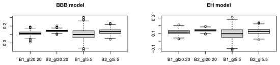
Figure 1. Boxplot for ${\widehat{\beta }}_{W1}$ and ${\widehat{\beta }}_{W2}$ in SRSS in the BBB model (left) and EH model (right).

The figure shows that the values of ${\widehat{\beta }}_{W2}$ are higher and the dispersion is lower than with ${\widehat{\beta }}_{W1}$ for all randomization methods. Moreover, the variance of the scramble variable increases in line with the dispersion.

Following this example, the value of the plug-in method based on the asymptotic variance, the jackknife and bootstrap variances and the dispersion obtained for each randomization method and degrees of freedom considered are represented by boxplot graphics (Figure 2).

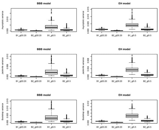
Figure 2. Boxplot for AV, JK and BS variances of ${\widehat{\beta }}_{W1}$ and ${\widehat{\beta }}_{W2}$ in SRSS in the BBB and EH models.

For each randomization method, we note that the greater the variance of the scramble variable S, the greater the dispersion. This behaviour is especially noticeable in the estimation of parameter ${\widehat{\beta }}_{W1}$. This result is expected, since adding more noise makes the dispersion increase, but in practice it is not possible to use scramble variables with little variance, as this reduces the privacy protection obtained.

To compare regression-based RR model and ratio-based RR model, we conducted the third simulation study in which both models are included. We use as sampling design the simple random sampling under a population of size $N=10,000$. Three different combinations of sample sizes were drawn from the population, $n=250,500,750$. As in the previous study, point estimators of the coefficient of regression were computed using the Eichhorn and Hayre (EH) and the Bar-Lev, Bobovitch and Boukai (BBB) models. A $F_{20,20}$ distribution was used for the scramble variable S, and in the BBB model $p=0.5$ was assumed. The main variable y and an auxiliary variables x were generated using the model $y_i=\beta x_i+{ϵ}_i$ with $E\left({ϵ}_i\right)={\sigma }^2{x}_i$, in this case $x\sim N(30,2)$, $\sigma =0.5$, $\beta =7$ and ${ϵ}_i\sim N(0,{\sigma }^2{x}_i)$.

For all randomization methods and in both models, regression and ratio, we can see (Table 3) how the values obtained from the relative bias and the relative mean squared error are small. Focusing on the RMSE, we observe that the value decreases as the sample size increases, as we expected, and we obtain a slightly better behavior of the ratio model compared to the regression model.

Table 3. Absolute relative bias and relative mean squared error in percent for ${\widehat{\beta }}_R$ and ${\widehat{\beta }}_W$ in SRS for the BBB and EH models.

	BBB Method				EH Method
	${\widehat{\mathbf{\beta }}}_{\mathbf{R}}$		${\widehat{\mathbf{\beta }}}_{\mathbf{W}}$		${\widehat{\mathbf{\beta }}}_{\mathbf{R}}$		${\widehat{\mathbf{\beta }}}_{\mathbf{W}}$
n	|RB|	RMSE	|RB|	RMSE	|RB|	RMSE	|RB|	RMSE
250	0.042	0.090	0.083	0.092	0.083	0.050	0.085	0.051
500	0.128	0.047	0.158	0.048	0.132	0.026	0.129	0.027
750	0.168	0.029	0.201	0.030	0.119	0.016	0.116	0.017

5. Real Application

As a real application of the methods described above, we conducted a survey by stratified random sampling at the University of *** to investigate the consumption of alcohol and drugs among the university population (in a sample of 754 students).

The sensitive question in this case was, “Indicates the age at which you started drinking alcohol and using drugs” and the RR technique used was the model proposed by [11]. To apply this model, each student was asked to use used as a randomizing device the app “Baraja Española” (a deck of cards, composed of 40 cards, divided into four families or suits, each numbered one to seven plus three face cards). When the user touches the screen, a card is shown. When it is a face card, the sensitive question should be answered; otherwise, the real number should be given, multiplied by the number shown on the card. Thus, the design parameter of the BarLev model was 3/10.

After the study data was compiled, a regression model was performed, in which the sensitive variable was taken as the dependent variable and the variable “Indicate on a scale of 0 (very bad) to 10 (optimal), how would you rate your relationship with your parents?” was an independent variable. After obtaining the value of the parameter, the estimate of the variance was obtained by the jackknife technique and the corresponding 95% confidence interval. This approach produced the following results:

$$\widehat{\beta }=2.392682,{\widehat{v}}_J(\widehat{\beta })=9.45795e^{-06}\mathrm{and}IC=[2.387;2.399].$$

In other words, the better the relationship with their parents, the higher the age at which these students began to consume alcohol and drugs.

6. Conclusions

Indirect interview techniques effectively reduce voluntary bias in surveys referring to sensitive questions. In recent years, many new techniques emerged for the estimation of proportions, means or totals of sensitive variables, but few studies addressed the question of dependency parameters.

In this paper, we propose a general scheme for a randomized response (RR) technique, under a general sampling design for estimating regression coefficients. We study the theoretical properties of the proposed estimators and we derive several estimators for their variances.

To assess the accuracy of the proposed estimators, a simulation study was conducted using two RR techniques. In this simulation study, the proposed estimators obtained good results in terms of relative bias and relative mean squared error.

The application of the proposed technique to a real survey enabled us to relate the age at which young people begin to consume alcohol and drugs with the perceived quality of the relationship with their parents.

References

- Arnab, R. Randomized response trials: A unified approach for qualitative data. Commun. Stat. Theory Methods 1996, 25, 1173–1183. [Google Scholar] [CrossRef]
- Barabesi, L.; Marcheselli, M. A practical implementation and Bayesian estimation in Franklin’s randomized response procedure. Commun. Stat. Simul. Comput. 2006, 35, 563–573. [Google Scholar] [CrossRef]
- Barabesi, L. A design-based randomized response procedure for the estimation of population proportion and sensitivity level. J. Stat. Plan. Inference 2008, 138, 2398–2408. [Google Scholar] [CrossRef]
- Perri, P. Modified randomized devices for Simmons’ model. Model Assist. Stat. Appl. 2008, 3, 233–239. [Google Scholar] [CrossRef]
- Lee, C.; Sedory, S.; Singh, S. Estimating at least seven measures of qualitative variables from a single sample using randomized response technique. Stat. Probab. Lett. 2013, 83, 399–409. [Google Scholar] [CrossRef]
- Liu, Y.; Tian, G. Multi-category parallel models in the design of surveys with sensitive questions. Stat. Interface 2013, 6, 137–142. [Google Scholar] [CrossRef]
- Greenberg, B.; Kuebler, R.; Abernathy, J.; Horvitz, D. Application of the randomized response technique in obtaining quantitative data. J. Am. Stat. Assoc. 1971, 66, 243–250. [Google Scholar] [CrossRef]
- Eriksson, S. A new model for randomized response. Int. Stat. Rev. 1973, 41, 40–43. [Google Scholar] [CrossRef]
- Pollock, K.; Bek, Y. A comparison of three randomized response models for quantitative data. J. Am. Stat. Assoc. 1976, 71, 884–886. [Google Scholar] [CrossRef]
- Eichhorn, B.; Hayre, L. Scrambled randomized response methods for obtaining sensitive quantitative data. J. Stat. Plan. Inference 1983, 7, 307–316. [Google Scholar] [CrossRef]
- Bar-Lev, S.; Bobovitch, E.; Boukai, B. A note on randomized response models for quantitative data. Metrika 2004, 60, 255–260. [Google Scholar] [CrossRef]
- Gjestvang, R.; Singh, S. A new randomized response model. J. R. Stat. Soc. B 2006, 68, 523–530. [Google Scholar] [CrossRef]
- Saha, A. A simple randomized response technique in complex surveys. Metron 2007, LXV, 59–66. [Google Scholar]
- Singh, S.; Kim, J. A pseudo-empirical log-likelihood estimator using scrambled responses. Statist. Probab. Lett. 2007, 81, 345–351. [Google Scholar] [CrossRef]
- Huang, K. Estimation for sensitive characteristics using optional randomized response technique. Qual. Quant. 2008, 42, 679–686. [Google Scholar] [CrossRef]
- Bouza, C. Ranked set sampling and randomized response procedures for estimating the mean of a sensitive quantitative character. Metrika 2009, 70, 267–277. [Google Scholar] [CrossRef]
- Diana, G.; Perri, P. A new scrambled response models for estimating the mean of a sensitive quantitative character. J. Appl. Stat. 2010, 37, 1875–1890. [Google Scholar] [CrossRef]
- Diana, G.; Perri, P. Calibration-based approach to sensitive data: A simulation study. J. Appl. Stat. 2012, 39, 53–65. [Google Scholar] [CrossRef]
- Gupta, S.; Shabbir, J.; Sehra, S. Mean and sensitivity estimation in optional randomized response models. J. Stat. Plan. Inference 2010, 140, 2870–2874. [Google Scholar] [CrossRef]
- Odumade, O.; Singh, S. An alternative to the Bar-Lev, Bobovitch, and Boukai randomized response model. Sociol. Methods Res. 2010, 20, 1–16. [Google Scholar] [CrossRef]
- Arcos, A.; Rueda, M.; Singh, S. A generalized approach to randomised response for quantitative variables. Qual. Quant. 2015, 49, 1239–1256. [Google Scholar] [CrossRef]
- Fox, J.; Tracy, P. Randomized Response: A Method for Sensitive Survey; Sage Publication, Inc.: Thousand Oaks, CA, USA, 1986. [Google Scholar]
- Chaudhuri, A.; Mukerjee, R. Randomized Response: Theory and Techniques; Marcel Dekker, Inc.: New York, NY, USA, 1988. [Google Scholar]
- Chaudhuri, A. Randomized Response and Indirect Questioning Techniques in Surveys; Chapman & Hall: London, UK, 2011. [Google Scholar]
- Chaudhuri, A.; Christofides, T. Indirect Questioning in Sample Surveys; Springer: Berlin/Heidelberg, Germany, 2013. [Google Scholar]
- Chaudhuri, A.; Christofides, T.; Rao, C. Data Gathering, Analysis and Protection of Privacy through Randomized Response Techniques: Qualitative and Quantitative Human Traits; Elsevier: Amsterdam, The Netherlands, 2016; Volume 34. [Google Scholar]
- Scheers, N.; Dayton, C. Improved estimation of academic cheating behavior using the randomized response technique. Res. High. Educ. 1987, 26, 61–69. [Google Scholar] [CrossRef]
- Blair, G.; Imai, K.; Zhou, Y. Design and Analysis of randomized response technique. J. Am. Stat. Assoc. 2005, 110, 1304–1319. [Google Scholar] [CrossRef]
- Van den Hout, A.; van der Heijden, P.; Gilchrist, R. The logistic regression model with response variables subject to randomized response. Comput. Stat. Data Anal. 2007, 51, 6060–6069. [Google Scholar] [CrossRef]
- Fox, J.; Veen, D.; Klotzke, K. Generalized Linear Mixed Models for Randomized Responses. Methodology 2019, 15, 1–18. [Google Scholar] [CrossRef]
- Hsieh, S.; Lee, S.; Shen, P. Logistic regression analysis of randomized response data with missing covariates. J. Stat. Plan. Inference 2010, 140, 927–940. [Google Scholar] [CrossRef]
- Singh, S.; Joarder, A.; King, M. Regression analysis using scrambled response. Aust. N. Z. J. Stat. 1996, 38, 201–211. [Google Scholar] [CrossRef]
- Van der Hout, A.; Kooiman, P. Estimating the linear regression model with categorical covariates subject to randomized response. Comput. Stat. Data Anal. 2006, 50, 3311–3323. [Google Scholar] [CrossRef]
- Arnab, R. Non-negative variance estimator in randomized response surveys. Commun. Stat. Theory Method 1994, 23, 1743–1752. [Google Scholar] [CrossRef]
- Barabesi, L.; Diana, G.; Perri, P. Design-based distribution function estimation for stigmatized populations. Metrika 2013, 76, 919–935. [Google Scholar] [CrossRef]
- Hájek, J. Comment on An essay on the logical foundations of survey sampling by Basu, D. In Foundations of Statistical Inference; Godambe, V.P., Sprott, D.A., Eds.; Springer: Berlin/Heidelberg, Germany, 1971. [Google Scholar]
- Särndal, C.E.; Swensson, B.; Wretman, J. Model Assisted Survey Sampling (Springer Series in Statistics); Springer: Berlin/Heidelberg, Germany, 1992. [Google Scholar]
- Binder, D. On the Variances of Asymptotically Normal Estimators from Complex Surveys. Int. Stat. Rev. Rev. Int. Stat. 1983, 51, 279–292. [Google Scholar] [CrossRef]
- Lumley, T. Package ‘survey’: Analysis of Complex Survey Samples. Available online: https://cran.r-project.org/web/packages/survey/index.html (accessed on 15 December 2020).
- Tukey, J. Bias and confidence in not-quite large samples. Ann. Math. Stat. 1958, 29, 614. [Google Scholar]
- Efron, B. Bootstrap methods: Another look at the jackknife. Ann. Stat. 1979, 7, 1–26. [Google Scholar] [CrossRef]
- Wolter, K. Introduction to Variance Estimation; Springer: Berlin/Heidelberg, Germany, 2007. [Google Scholar]
- Arnab, R.; Cobo, B. Variance jackknife estimation for randomized response surveys: A simulation study and an application to explore cheating in exams and bullying. Comput. Math. Methods 2020, 2, e1073. [Google Scholar] [CrossRef]
- Rueda, M.; Cobo, B.; Perri, P.F. Randomized response estimation in multiple frame surveys. Int. J. Comput. Math. 2020, 97, 189–206. [Google Scholar] [CrossRef]
- Booth, J.; Butler, R.; Hall, P. Bootstrap methods for finite populations. J. Am. Stat. Assoc. 1994, 89, 1282–1289. [Google Scholar] [CrossRef]
- Antal, E.; Tillé, Y. A direct bootstrap method for complex sampling designs from a finite population. J. Am. Stat. Assoc. 2011, 106, 534–543. [Google Scholar] [CrossRef]
- Antal, E.; Tillé, Y. A new resampling method for sampling designs without replacement: The doubled half bootstrap. Comput. Stat. 2014, 29, 1345–1363. [Google Scholar] [CrossRef]
- Zhao, P.; Haziza, D.; Wu, C. Survey weighted estimating equation inference with nuisance functionals. J. Econom. 2020, 216, 516–536. [Google Scholar] [CrossRef]
- Wu, C.; Thompson, M.E. Resampling and Replication Methods. In Sampling Theory and Practice. ICSA Book Series in Statistics; Springer: Berlin/Heidelberg, Germany, 2020. [Google Scholar] [CrossRef]
- Goldfeld, K. Package ‘simstudy’: Simulation of Study Data. Available online: https://cran.r-project.org/web/packages/simstudy/index.html (accessed on 15 December 2020).
- Tillé, Y.; Matei, A. Package ‘sampling’: Survey Sampling. Available online: https://cran.r-project.org/web/packages/sampling/index.html (accessed on 15 December 2020).
Publisher’s Note: MDPI stays neutral with regard to jurisdictional claims in published maps and institutional affiliations. |
© 2021 by the authors. Licensee MDPI, Basel, Switzerland. This article is an open access article distributed under the terms and conditions of the Creative Commons Attribution (CC BY) license (http://creativecommons.org/licenses/by/4.0/).