A Mathematical Model of Contact Tracing during the 2014–2016 West African Ebola Outbreak

Abstract

The 2014–2016 West African outbreak of Ebola Virus Disease (EVD) was the largest and most deadly to date. Contact tracing, following up those who may have been infected through contact with an infected individual to prevent secondary spread, plays a vital role in controlling such outbreaks. Our aim in this work was to mechanistically represent the contact tracing process to illustrate potential areas of improvement in managing contact tracing efforts. We also explored the role contact tracing played in eventually ending the outbreak. We present a system of ordinary differential equations to model contact tracing in Sierra Leonne during the outbreak. Using data on cumulative cases and deaths, we estimate most of the parameters in our model. We include the novel features of counting the total number of people being traced and tying this directly to the number of tracers doing this work. Our work highlights the importance of incorporating changing behavior into one’s model as needed when indicated by the data and reported trends. Our results show that a larger contact tracing program would have reduced the death toll of the outbreak. Counting the total number of people being traced and including changes in behavior in our model led to better understanding of disease management.

1. Introduction

In March 2014, the most deadly outbreak to date of Ebola virus disease (EVD), a hemorrhagic fever, began in Guinea and rapidly spread to Liberia, Nigeria, Senegal, and Sierra Leone [1]. In October 2014, the World Health Organization (WHO) Ebola Response Team estimated an overall case fatality rate of $70.8\%$ and basic reproduction numbers (${\Re }_0$) of $1.71$ for Guinea, $1.83$ for Libera and $1.38$ for Sierra Leone [2]. Concern that Ebola might spread globally via airline travel led to recommendations for health assessments at airports in the affected countries [3]. A review and meta-analysis of 31 reports found that the main methods of spread were direct contact with an infected individual and contact with deceased loved ones during traditional funeral practices [4]. In the 2014–2016 outbreak in Sierra Leone, among individuals confirmed to have EVD, $47.9\%$ reported that they had had contact with someone suspected of having EVD, and $25.5\%$ reported having attended a funeral [5]. These transmission pathways are further indicated as important by mathematical models and by statistical models [6,7,8,9]. Ebola can survive on some surfaces for up to 192 h unless they are properly disinfected [10]. This might be one of the reasons why so many health care workers became infected [11]. Outcomes for individuals who contracted EVD during the outbreak varied based on location, time of infection, and whether the individual was hospitalized [12].

Contact tracing, sometimes called partner notification, is often used in the fight against the spread of HIV (Human Immunodeficiency Virus) [13,14,15]. Contact tracing for Ebola is quite different, though, because it does not focus primarily on sexual partners but rather on people who have been in some kind of close contact with the infected or deceased individual. The goal of contact tracing is to identify secondary infections and to isolate them in order to stop disease transmission. Throughout the outbreak, the Centers for Disease Control and Prevention’s Morbidity and Mortality Weekly Report detailed the progress of the disease as well as some information about contact tracing efforts. The ideal process for contact tracing is now described, though in some cases it was altered due to constraints of geography, resource limitations, or testing availability. Contacts were traced for 21 days after their last known exposure to a confirmed, probable, or suspected case [16]. All contacts being traced were instructed to remain isolated from the general population. If a contact showed symptoms of EVD, they were moved to a suspected case isolation ward and tested. If the test was positive, that individual was moved to the confirmed case ward. If the test was negative, the individual was sent home to be traced for another 21 days.

Webb and Browne and their collaborators built two models using data from Sierra Leone and Guinea [17,18]. In their SEIR (Susceptible–Exposed–Infectious–Recovered) model [17], they incorporated contact tracing by building separate compartments for Exposed individuals and Infectious individuals being traced. Their model did not include spread within hospitals and spread from contact with deceased individuals. They found that increasing the fraction of cases reported and increasing the fraction of reported contacts that were traced could bring ${\Re }_0$ below 1. They also provided weekly point estimates for the effective reproduction number for Guinea and Sierra Leone. In [18], they had a system of ODEs and a corresponding stochastic model implementation, which included a compartment for improperly buried bodies of infectious individuals, but did not include a hospitalized compartment and did not include the workload of tracing persons who do not become infected. In this work, we will use a similar, but more mechanistic approach of counting persons being traced and accounting for the workload of the contact tracers. Our model will include compartments for hospitalized individuals and for dead bodies from improper burials.

Rivers et al. [19] built an SEIR model of the epidemic in Sierra Leone and Liberia while it was ongoing and before it had reached a peak. They concluded that improved contact tracing could have a large impact on number of cases but that even when combined with two other interventions contact tracing was insufficient to bring the epidemic to an end. They identified the duration of a traditional funeral in Sierra Leone as 4.5 days and the length of the incubation period as 10 days—values which we use in our model. Their work represented improved contact tracing implicitly by increasing the proportion of infected cases that are diagnosed and hospitalized and decreasing the time it takes for an infected individual to be hospitalized (from a baseline scenario), but our model will illustrate contact tracing more explicitly by counting the number of persons being traced. This counting will indicate the people resources needed for the tracing process, not just the effects of the tracing.

In Sierra Leone, contact tracing was hampered by practical difficulties [20]. Olu et al. analyzed contact tracing interview data in the western area districts of Sierra Leone [21], and noted that contact tracing was hindered by under-reporting of exposure, political difficulties in hiring tracers, and an incomplete database for use of tracers. Contacts being traced were supposed to be provided with basic needs, such as food and water, but this often did not occur. Some contacts were difficult to trace because of the stigma of being listed as a contact, and the average number of contacts per case was only 8.5 which was lower than in comparable situations. Olu et al. found that some people gave false information to tracers, withheld information from tracers, and communities tended not to trust tracers. This resulted in missed contacts. According to field staff (personal communication, Centers for Disease Control and Prevention) [22], there were difficulties in procuring additional people to perform contact tracing. In an urban area, a tracer could trace about 15 individuals per day, while in a rural area, a tracer could trace 10 individuals per day. In January 2015, there were 1200 contact tracers in Western Area, Sierra Leone. In neighboring Liberia, tracers faced difficulty finding contacts, difficulty with completing all 21 days of tracing, and resistance of symptomatic contacts to report to an Ebola Treatment Unit (ETU) [23]. Other challenges faced by contact tracers in Liberia included contacts hiding from tracers, people failing to identify all contacts or lying about their own exposure, resistance to in-home isolation, and difficulties in finding contact tracers. Many of the same problems were encountered in Sierra Leone. A study by Swanson et al. found that contact tracing in Liberia was performed for $26.7\%$ of cases and only identified $3.6\%$ of new cases [24], suggesting room for improvement. Chowell and Nishiura [25] illustrated the insights for disease management that can come from modeling connected with Ebola epidemiological data and discussed the need for understanding the effectiveness of contact tracing.

Our goal was to carefully and mechanistically represent the contact tracing process to illustrate potential areas of improvement in managing contact tracing efforts. We explored the role contact tracing played in eventually ending the outbreak. Our model uses a novel feature, which is explicitly counting the people being traced and connecting the total persons traced with the workload of contact tracer workers. We will focus our model on Sierra Leone, for which we have data from the Sierra Leone Ministry of Health [26,27]. These data include cumulative confirmed cases and cumulative confirmed deaths as reported online during the outbreak in the daily situation report. We will design a system of Ordinary Differential Equations (ODEs) explicitly incorporating contact tracing, fit this model to our data, and see what insights we might gain from this mechanistic approach.

2. Model

Our model is a compartmental model made up of a system of ODEs and follows an SEIR approach, similar to [17,18,19,21,28]. In addition to the Susceptible, Exposed, Infected, and Recovered classes, we also include a class (D) to account for the persons who have died from Ebola in the community (i.e., having not been effectively isolated in a hospital or by other means), because they are a significant source of infection due to traditional funeral practices, such as hugging and kissing the body of a deceased loved one. We also include a Hospitalized (H) class, in which individuals are assumed to be isolated and not contribute to infection, and if they die their bodies are assumed to be disposed of safely. We place no upper limit on the size of class H, which does not reflect the situation during the outbreak where insufficient beds and staffing were a major limiting factor in controlling the outbreak [29], but allows us to examine the operation of a contact tracing system assuming hospital resources are readily available.

Our investigation of contact tracing begins with adding two new classes of individuals being traced. Since exposure is a hidden trait, individuals being traced are either susceptible or exposed. We created a class called F of susceptible individuals who are being traced but will not become ill and a second class, $E_F$, for individuals being traced who are exposed and will become infectious. Two events can lead to initiation of contact tracing: either an individual enters the D class or an individual enters the H class. The contacts connected to the individuals involved in either of these two events will be contacted each day for 21 days by a contact tracer. We assume that individuals in the F class being traced will follow isolation guidelines to prevent them from becoming exposed. Individuals in $E_F$ are moved to the hospital when they present symptoms. 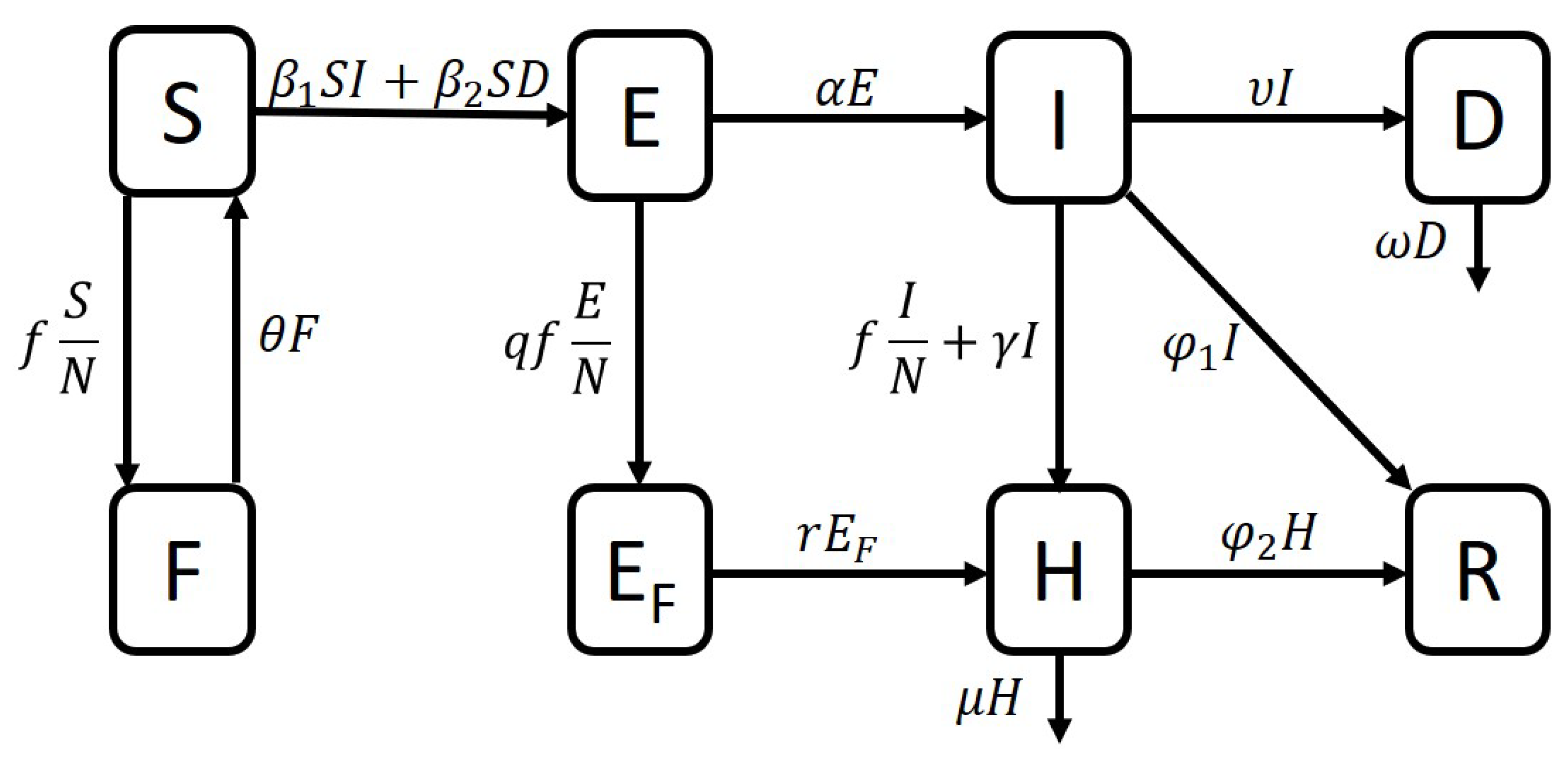The function f alters the completion rate of key contact tracing steps based on the amount of work to be done along with the number of available contact tracing staff. There is a limited number of contact tracers, and each contact tracer is able to trace a limited number of individuals at a time. To account for this, we place a threshold on the total number of contacts that can be traced at a time. Part of the work carried out by contact tracers is moving individuals to the hospital, and the remaining effort is dedicated to visiting contacts who have not (yet) displayed any symptoms of Ebola. In our flow diagram in Figure 1, one can see the terms with coefficient f representing the effects of contact tracing. Our model with eight compartments is below:

$$\begin{array}{cc}\hfill S^{\prime }& =-{\beta }_{1}SI-{\beta }_{2}SD-f{\displaystyle \frac{S}{N}}+\theta F\hfill \end{array}$$

(1)

$$\begin{array}{cc}\hfill F^{\prime }& =f{\displaystyle \frac{S}{N}}-\theta F\hfill \end{array}$$

(2)

$$\begin{array}{cc}\hfill E^{\prime }& ={\beta }_{1}SI+{\beta }_{2}SD-qf{\displaystyle \frac{E}{N}}-\alpha E\hfill \end{array}$$

(3)

$$\begin{array}{cc}\hfill E_F^{\prime }& =qf{\displaystyle \frac{E}{N}}-r{E}_F\hfill \end{array}$$

(4)

$$\begin{array}{cc}\hfill I^{\prime }& =\alpha E-f{\displaystyle \frac{I}{N}}-\gamma I-{\varphi }_{1}I-\nu I\hfill \end{array}$$

(5)

$$\begin{array}{cc}\hfill H^{\prime }& =r{E}_F+f{\displaystyle \frac{I}{N}}+\gamma I-{\varphi }_{2}H-\mu H\hfill \end{array}$$

(6)

$$\begin{array}{cc}\hfill R^{\prime }& ={\varphi }_{1}I+{\varphi }_{2}H\hfill \end{array}$$

(7)

$$\begin{array}{cc}\hfill D^{\prime }& =\nu I-\omega D\hfill \end{array}$$

(8)

where $N=S+E+I$. The function f depends on F, $E_F$, and I and gives the rate of finding new contacts

$$f=\left\{\begin{array}{cc}{\kappa }_1\gamma I+{\kappa }_2\nu I\hfill & \mathrm{if}F+E_F<\left(15\right)\left(1200\right)p\hfill \\ 0\hfill & \mathrm{else}\hfill \end{array}\right..$$

(9)

Here, $1-p$ is the proportion of the total available contact tracing effort dedicated to hospitalizing individuals identified as symptomatic. Note that the two events (movement into H and D) can be seen in the function f with the rates $\gamma I$ and $\nu I$. In the cutoff for f, the number 15 is how many contacts on average one contact tracer can trace, and the number 1200 is the maximum number of contact tracers that were employed in the Western Area, Sierra Leone (containing the capital city of Freetown), during the 2014–2016 epidemic [22]. Although the total number of contact tracers varied throughout the outbreak, we decided to assume the maximum of 1200 was available throughout the outbreak. The units of f are persons per day. The units of each compartment are individuals. The units and interpretation of each parameter are listed in

Table 1. The parameters and compartment names in our model with their interpretations and units.

Symbol	Interpretation	Units
${\beta }_1$	transmission from interactions between I and S	per person per time
${\beta }_2$	transmission from interactions between D and S	per person per time
$1/\theta$	number of days a person is traced	time
$1/\alpha$	length of the exposed period	time
r	rate of hospitalization for traced individuals	per time
$\gamma$	rate of hospitalization for untraced individuals	per time
${\varphi }_1$	recovery rate for untreated	per time
${\varphi }_2$	recovery rate for treated	per time
$\nu$	death rate for untreated	per time
$\mu$	death rate for treated	per time
$\omega$	rate at which dead bodies become non-infectious	per time
${\kappa }_1$	contacts recruited from hospitalization of one person	unitless
${\kappa }_2$	contacts recruited from funeral of one person	unitless
q	scaling factor for exposed contacts	unitless
S	susceptibles	individuals
F	susceptibles being traced	individuals
E	exposed	individuals
$E_F$	exposed being traced	individuals
I	infectious	individuals
H	hospitalized	individuals
D	dead bodies	individuals
R	recovered	individuals

. Note that we do not account for births or for deaths from any other cause than Ebola.

People can move from Susceptible to Exposed by coming into contact with a member of the Infectious class (term ${\beta }_{1}SI$) or by coming into contact with an infectious dead body (term ${\beta }_{2}DS$). People who are being traced move from Susceptible to F or from Exposed to $E_F$ by coming into contact with a person who has just been hospitalized or attending a funeral for somebody who has just died of Ebola (term $f\frac{S}{N}=({\kappa }_1\gamma I+{\kappa }_2\nu I)\frac{S}{N}$). This term is scaled by N because the persons moving in tracing are moved proportionally to the ratio of persons in their current class. For example, a person being traced from S moves to F at a rate proportional to $\frac{S}{N}=\frac{S}{S+E+I}$. A person is more likely to be in $E_F$ while being traced than to be in F because of the contact they had with either an infected person or a dead body. To account for this, we multiply the term $f\frac{E}{N}$ by a number $q>1$, a scaling factor to increase the likelihood of $E_F^{\prime }s$ being traced relative to that of $F^{\prime }s$ being traced. People who have completed their time being traced and have not developed symptoms move back into S (term $\theta F$). Once a person has been in the Exposed class for an average of 10 days, they move to the Infectious class (term $\alpha E$). A person in the class $E_F$ is moved to the hospital once they develop symptoms (term $r{E}_F$). If an individual being traced shows symptoms the first time they are contacted, they are immediately moved to the hospital (term $f\frac{I}{N}$). Some Infectious people decide to go to the hospital on their own (term $\gamma I$). Some Infectious people manage to survive Ebola and move to R (term ${\varphi }_{1}I$) but others die of the disease and we assume they are not safely buried and contribute to the class D (term $\nu I$). This is a simplifying assumption, because, as the epidemic drew on, many people who died in the community were safely buried. Some Hospitalized individuals will recover (term ${\varphi }_{2}H$) but others will die and be safely buried (term $\mu H$). After some time has passed, an unsafely buried dead body is no longer able to infect people (with decay term $\omega D$).

3. Reproductive Number

We will derive the basic reproductive number ${\Re }_0$ using the standard method of the Next Generation Matrix [30,31,32,33]. We expect that near the disease-free equilibrium (DFE), the number of infections will be small but non-zero. The population affected by the outbreak consisted entirely of susceptibles at the beginning of the outbreak. Therefore, for this analysis, we assume that $f={\kappa }_1\gamma I+{\kappa }_2\nu I$.

Now, Equation (7) implies

$${\varphi }_1{I}^{\ast }=-{\varphi }_2{H}^{\ast }.$$

(10)

Giving $I^{\ast }=H^{\ast }=0$. From Equation (8), we get $D^{\ast }=0$. Since $I^{\ast }=0$, Equation (2) gives $F^{\ast }=0$ and Equation (5) gives $E^{\ast }=0$. Since $I^{\ast }=H^{\ast }=0$, Equation (6) gives $E_F^{\ast }=0$. Since $E^{\ast }=I^{\ast }=0$, we conclude that $S^{\ast }=N\left(0\right)$. We have the DFE: $(S^{\ast },0,0,0,0,0,R^{\ast },0)$. However, we take $R^{\ast }=0$ for computation of the Next Generation Matrix. The diseased classes here are: E, $E_F$, I, H, and D, with corresponding vectors $\mathcal{F}-\mathcal{V}$ forming the right hand side of the system with only diseased classes,

$$\mathcal{F}=\left(\begin{array}{c}{\beta }_{1}SI+{\beta }_{2}SD\\ 0\\ 0\\ 0\\ 0\end{array}\right),\mathcal{V}=\left(\begin{array}{c}\alpha E+q({\kappa }_1\gamma I+{\kappa }_2\nu I)\frac{E}{S+I+E}\\ r{E}_F-q({\kappa }_1\gamma I+{\kappa }_2\nu I)\frac{E}{S+I+E}\\ ({\varphi }_1+\nu +\gamma )I+({\kappa }_1\gamma I+{\kappa }_2\nu I)\frac{I}{S+I+E}-\alpha E\\ ({\varphi }_2+\mu )H-r{E}_F-\gamma I-\frac{({\kappa }_1\gamma +{\kappa }_2\nu )I^2}{S+I+E}\\ \omega D-\nu I\end{array}\right).$$

It is easy to show that our model satisfies the assumptions required for use of the Next Generation Method. Note that our DFE is not unique and this is not required. We get the Jacobian matrices $D\mathcal{F}(E,E_F,I,H,D)$ and $D\mathcal{V}(E,E_F,I,H,D)$ at the DFE, $(0,0,0,0,0)$ with $S=S^{\ast }$,

$$\begin{array}{ccc}\hfill D\mathcal{F}(0,0,0,0,0)& =& \left(\begin{array}{ccccc}0& 0& {\beta }_1{S}^{\ast }& 0& {\beta }_2{S}^{\ast }\\ 0& 0& 0& 0& 0\\ 0& 0& 0& 0& 0\\ 0& 0& 0& 0& 0\\ 0& 0& 0& 0& 0\end{array}\right),\hfill \\ \hfill D\mathcal{V}(0,0,0,0,0)& =& \left(\begin{array}{ccccc}\alpha & 0& 0& 0& 0\\ 0& r& 0& 0& 0\\ -\alpha & 0& {\varphi }_1+\nu +\gamma & 0& 0\\ 0& -r& -\gamma & {\varphi }_2+\mu & 0\\ 0& 0& -\nu & 0& \omega \end{array}\right).\hfill \end{array}$$

Thus, the basic reproductive number we obtain as the spectral radius of the matrix $D\mathcal{F}(0,0,0,0,0){\left(D\mathcal{V}\right)}^{-1}(0,0,0,0,0)$ is

$${\Re }_0={\displaystyle \frac{{\beta }_1{S}^{\ast }}{{\varphi }_1+\nu +\gamma }}+{\displaystyle \frac{\nu {\beta }_2{S}^{\ast }}{\omega ({\varphi }_1+\nu +\gamma )}}.$$

(11)

The first term describes the number of new infections that we expect per individual from the I class, and the second term describes the number of new infections that we expect per body in the D class.

4. Parameter Estimation

Our data are taken from the Sierra Leone Ministry of Health daily situation reports, published on their website during the epidemic. We accessed these old web sites via the Wayback Machine at https://web.archive.org/web/20150314233800/http:/health.gov.sl/?page_id=583 (accessed on 28 February 2020). Data are listed in Appendix A. Situation reports were available beginning at Day 77 with the final day being Day 504, but not every intermediate day had a report. There were 343 total reports available for us to use. From these reports, we used confirmed cases and deaths. There was one report we chose to exclude because it listed more confirmed deaths than subsequent reports, making our total number of data points 342.

We chose some parameters from the literature and estimated others using our data. The parameters

$$\alpha =0.1,\frac{1}{\omega }=4.5,\frac{1}{\theta }=21$$

were taken from the literature [16,19,21,28]. Our data indicated that the initial condition for the H class was $H\left(0\right)=94$ individuals. We assumed the initial condition for the recovered class was $R\left(0\right)=0$ individuals, and that the initial condition for S was roughly equivalent to the population of Sierra Leone at the time, $S\left(0\right)=$ 6,348,350 people. We estimated the following parameters:

$${\beta }_1,{\beta }_2,\gamma ,{\kappa }_1,{\kappa }_2,r,p,\nu ,\mu ,{\varphi }_1,{\varphi }_2.$$

We estimated the following initial conditions:

$$F\left(0\right),E\left(0\right),E_F\left(0\right),I\left(0\right),D\left(0\right).$$

See Table 1 for parameter interpretations and units.

We estimated the above parameters in MATLAB using multistart to generate many vectors of starting parameter estimates. Each vector was used to initialize a search in fmincon, which is a local minimizer. In MATLAB ode45 served as our ODE solver. Parameter upper and lower bounds were based on ranges of parameters from the literature [19,21] and from our data. We used papers [19,21] for some ranges because they rely on data from Sierra Leone. For example, parameters comparable to our ${\beta }_1$, ${\beta }_2$, ${\varphi }_1$, and ${\varphi }_2$ were found in Rivers [19]. Our lower limit for r was based on both papers [19,21]. There is also a parameter in Olu comparable to our parameter ${\kappa }_1$ [21]. For example, the upper bound for $F_0$ was taken as 2500 because our data indicated that in early days this was roughly the number of contacts being traced. To estimate our cumulative simulated cases, we summed over the entries into the H class, assuming that cases for people in the community were unconfirmed. To estimate our cumulative simulated deaths, we summed over the deaths from H and I together. The data to be compared with simulation results are cumulative confirmed cases and cumulative confirmed deaths. We minimized the following:

$$J=\sum _{i=77}^{504}\left(\frac{{({\mathrm{Cases}}_{Estimated}\left(i\right)-{\mathrm{Cases}}_{Data}\left(i\right))}^2}{{\left({\mathrm{Cases}}_{Data}\left(i\right)\right)}^2}+\frac{{({\mathrm{Deaths}}_{Estimated}\left(i\right)-{\mathrm{Deaths}}_{Data}\left(i\right))}^2}{{\left({\mathrm{Deaths}}_{Data}\left(i\right)\right)}^2}\right),$$

(12)

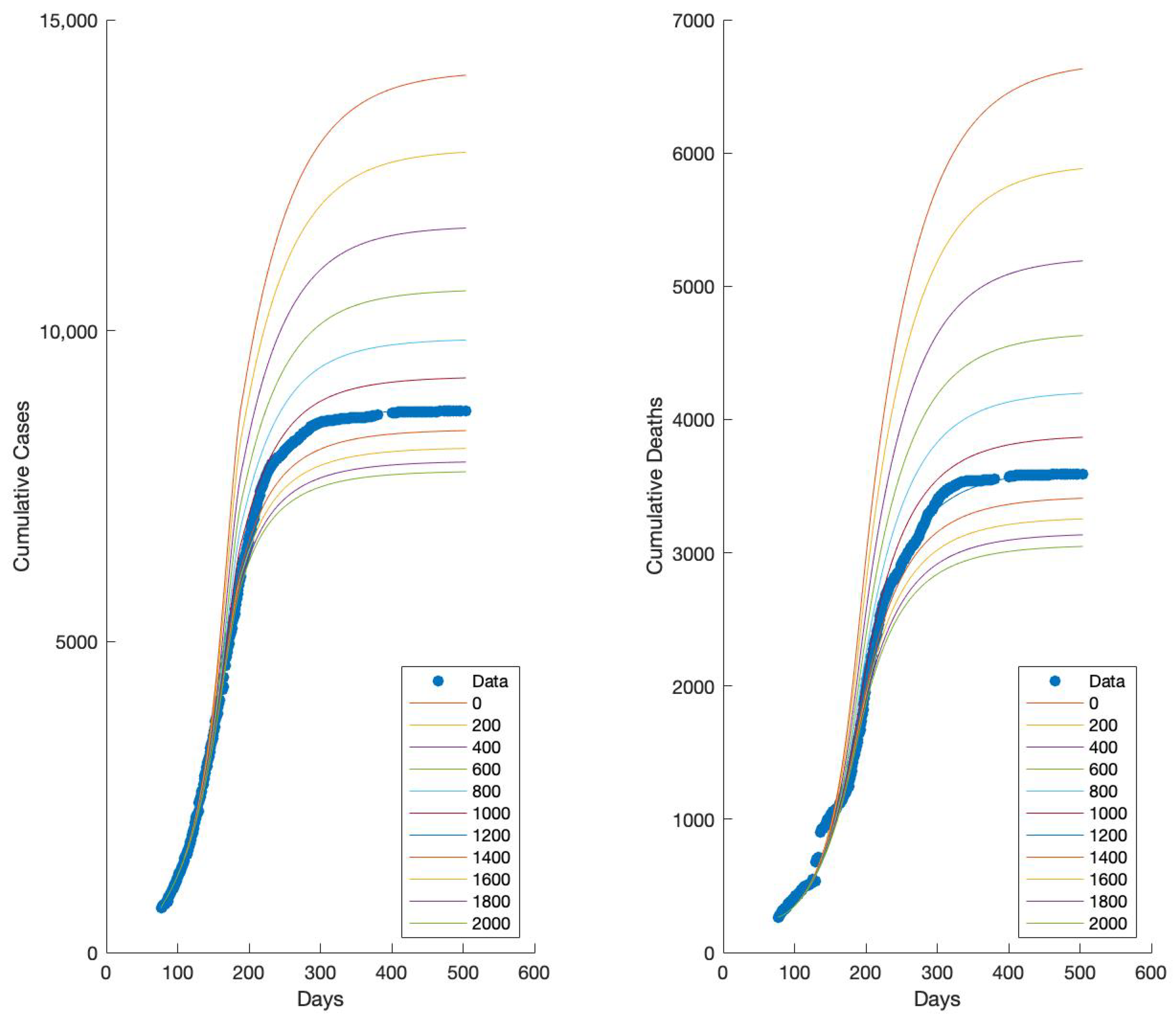
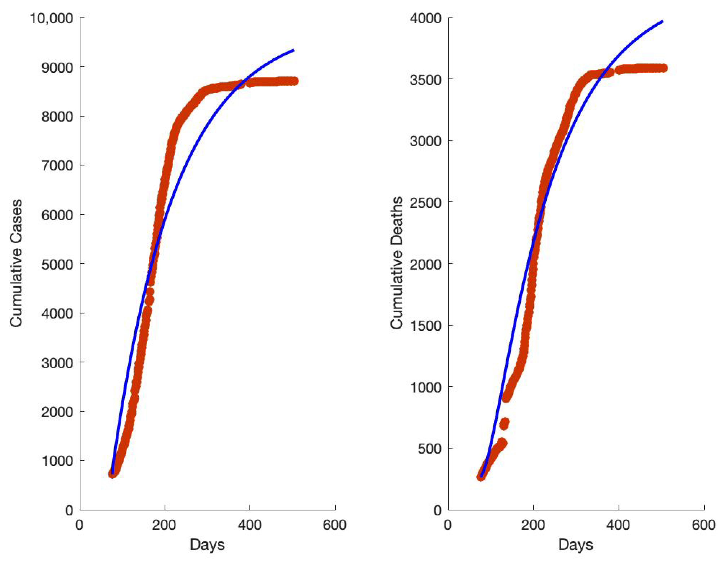
which is a type of sum of least squares for our model. Our data began at day 77 and ended at day 504, with 342 total data points each for cases and deaths. Note that this does not include every day between day 77 and day 504. The missing data are for days when the Ministry of Health situation report was unavailable. The data from one day, when cumulative deaths were higher than for following days, were excluded. You can see that some days do not have data by the gaps in the red dots in Figure 2.

We had two primary goals during the process of parameter estimation:

• Fit the data with a low J value;
• In each class, we wanted reasonable dynamics, meaning approximately the correct magnitude in the size of each compartment.

We tried several ways of fitting the data. First, we estimated all the parameters listed above, holding them all constant throughout the epidemic. This resulted in simulated epidemic curves that did not flatten at the end, indicating the epidemic would have kept going (see Appendix B). Then, we chose five parameters that seemed to vary during the epidemic according to the literature and allowed those five parameters to switch from one value to a second value in the middle of the epidemic with a smoothed transition between the two values. In order to achieve a good simulation of the data with reasonable compartments, we modified the model by inserting the parameter q. Then, we reestimated the parameters using the varying approach for five of the parameters. This resulted in good simulations of the data with reasonable compartments.

In order to achieve a simulated fit of the data, which would include a flattening of the cumulative cases and cumulative deaths curves rather than simulations that indicated the epidemic would not have ended, we decided to allow some parameters (specifically ${\beta }_1,{\beta }_2,\gamma ,{\kappa }_1,$ and ${\kappa }_2$) to vary over the course of the epidemic. We chose these parameters because we knew that people’s behavior changed during the epidemic. We smoothed the transition from the first value of each of these parameters to the second value using piecewise functions such as the one below for each of the parameters

$${\beta }_1\left(t\right)=\left\{\begin{array}{cc}6.68\times {10}^{-8}\hfill & t<160\hfill \\ 6.68\times {10}^{-8}(1-\frac{t-160}{30})+3.94\times {10}^{-8}\left(\frac{t-160}{30}\right)\hfill & 160\le t\le 190\hfill \\ 3.94\times {10}^{-8}\hfill & t>190.\hfill \end{array}\right.$$

(13)

Chowell et al. [34] built a system of ODEs representing Ebola outbreaks in Congo and Uganda and used a smooth transition between two transmission rates due to control interventions (such as education and contact tracing followed by quarantine).

The literature supports our decision to allow ${\beta }_1,{\beta }_2,\gamma ,{\kappa }_1$ and ${\kappa }_2$ to change over the course of the epidemic. Senga et al. [28] analyzed data on probable and confirmed cases of EVD and their contacts in Kenema district, Sierra Leone, taken from the national database. They found that the number of contacts per case increased over time. The low number of contacts per case reported early in the epidemic was much lower than those reported in other countries, which they concluded meant that the contact listings were incomplete. Olu et al. found that during the months of June 2014 to November 2014 the average number of contacts per case was nine, and that during the months of December 2014 to May 2015, the average number of contacts per case increased to 16 [21]. Lokuge et al. reported that, later in the epidemic, people were more likely to come to the hospital of their own volition, less likely to report funeral contact, and that contact tracing increased in efficacy [29]. These findings from the literature indicate it is reasonable to conclude that values for ${\beta }_1,{\beta }_2,\gamma ,{\kappa }_1$ and ${\kappa }_2$ changed during the course of the epidemic due to changes in behavior and the level of education in the population about EVD.

However, we were unable to generate reasonable sizes for compartment $E_F$. Our simulations were showing very few people passing through $E_F$, which is not reflective of the success that contact tracing achieved in locating exposed individuals during the outbreak. We decided to modify the model by adding a multiplier, q, in front of the $f\frac{E}{N}$ term. We tried several values and found that a value of $q=100$ generated reasonable sizes for compartment $E_F$. This multiplier indicates that people who were being traced had had contact with an individual who was infectious or with a dead body, so they were more likely to have been exposed to Ebola than a member of the population who had not had such contact. These changes resulted in the simulations shown in Figure 2, Figure 3 and Figure 4 which were generated using the parameters found in

Table 2. Values for parameters, with five parameters having early and late values. Parameters with * were taken from the data or the literature. Others were estimated.

Parameter	Value	Parameter	Value
${\beta }_1$ early	$1.00\times {10}^{-9}$	r	$0.056$
${\beta }_1$ late	$1.00\times {10}^{-9}$	p	$0.90$
${\beta }_2$ early	$1.00\times {10}^{-6}$	$\nu$	$0.024$
${\beta }_2$ late	$1.00\times {10}^{-7}$	$\mu$	$0.010$
$\gamma$ early	$0.41$	${\varphi }_1$	$0.020$
$\gamma$ late	$0.062$	${\varphi }_2$	$0.028$
${\kappa }_1$ early	$29.74$	$F\left(0\right)$	$2451.10$
${\kappa }_1$ late	$44.93$	$E\left(0\right)$	$32.04$
${\kappa }_2$ early	$44.62$	$E_F\left(0\right)$	$124.88$
${\kappa }_2$ late	$16.61$	$I\left(0\right)$	$71.76$
		$D\left(0\right)$	$6.09$
${\alpha }^{\ast }$	$0.1$	$1/{\omega }^{\ast }$	$4.5$
$H{\left(0\right)}^{\ast }$	94	$S{\left(0\right)}^{\ast }$	$6,348,350$
$R{\left(0\right)}^{\ast }$	0	$1/{\theta }^{\ast }$	21

.

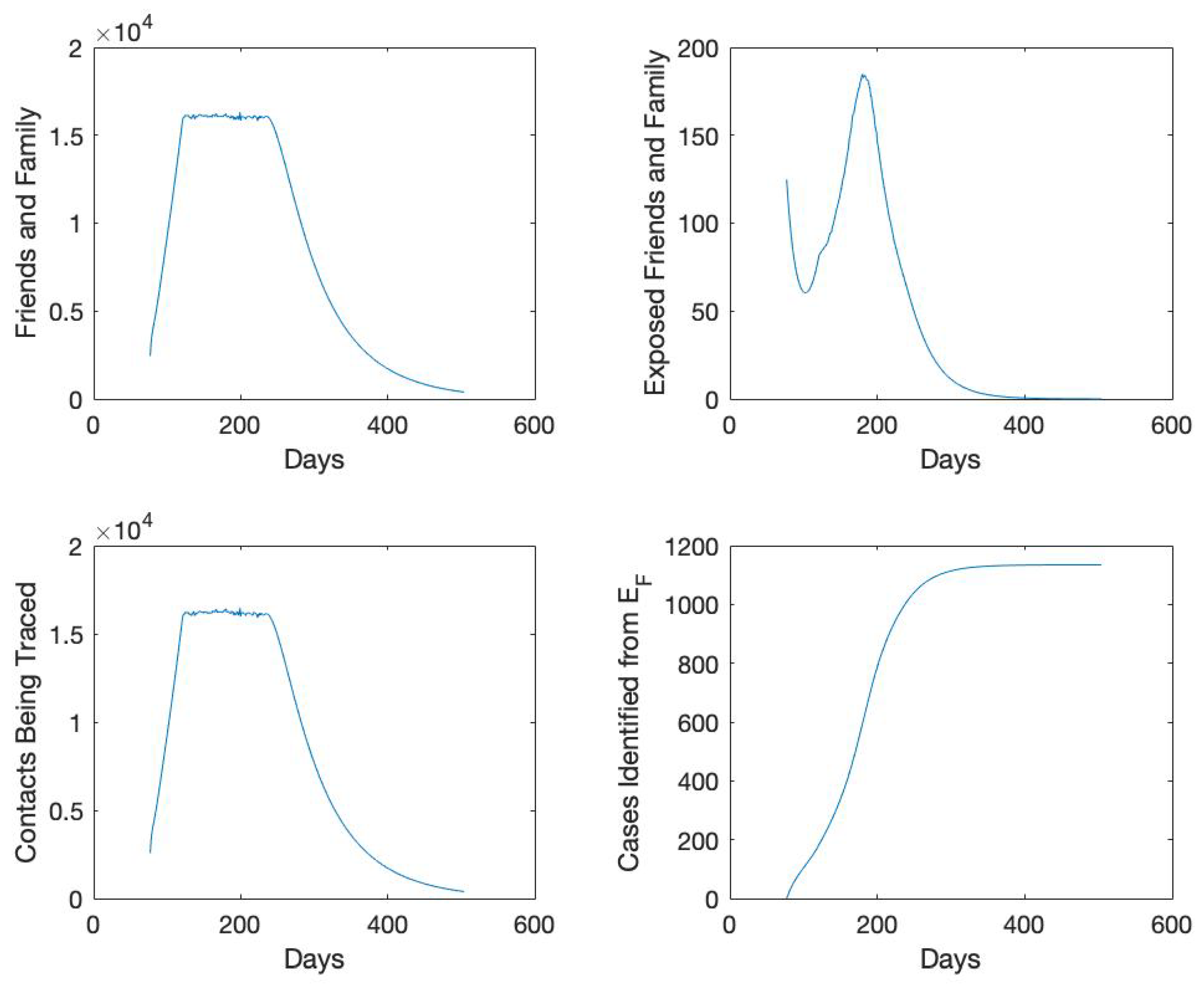
Figure 3 shows how many cases total were identified as part of the contact tracing effort. Near the end of the outbreak, this number reaches about 1100, which represents more than a tenth of all confirmed cases. This demonstrates the importance of successful contact tracing. The peak of contact tracing numbers corresponds to the slowing of the increase in cumulative cases, around day 200. This indicates that contact tracing efforts contributed to ending the epidemic.

Note that in Figure 4, the increase later in the epidemic of S results from people returning to S from F after being traced for 21 days and showing no symptoms. In Figure 4, the peak in E occurs at day 164, the peak in H about two weeks later on day 176, the peak in I about two weeks after that on day 192, and then the peak in D on day 197. It is not surprising that the peak in E precedes the other peaks, but it is surprising that the peak in D is the last peak to occur. This indicates that there may have been unsafely buried bodies later in the epidemic, but that fewer people were catching Ebola from funeral interactions despite this increase in funerals.

In Table 2, there is no difference between ${\beta }_1$ early and ${\beta }_1$ late. However, ${\beta }_2$ changes from an early value of $1.00\ast {10}^{-6}$ to a much lower later value of $1.00\ast {10}^{-7}$. These parameter values indicate that while the rate of transmission from interactions between S and I remained about the same throughout the epidemic, the rate of transmission from D to S decreased dramatically as people became more educated about Ebola. Oddly, $\gamma =0.41$ decreases to a later value of $\gamma =0.062$, which does not agree with accounts from the literature that people were more likely to come to the hospital once they developed symptoms later in the epidemic than they were earlier in the epidemic. The value of ${\kappa }_1=29.74$ early increases to ${\kappa }_1=44.93$ late, corresponding to reports from the literature that people were more likely to report more complete lists of contacts later in the epidemic. However, ${\kappa }_2=44.62$ early decreased to ${\kappa }_2=16.61$ late, adding to the conclusion that people were less likely to attend traditional funerals later in the epidemic. The changes in these parameters during the outbreak might be caused by a combination of factors, including educating the public about Ebola [35], increases in available beds at Ebola Treatment Centers, and more effective implementation of contact tracing.

The value of $r=0.056$ means that contacts who were infected took an average of 18 days to show symptoms. This value for r is probably unrealistically small, as it should likely be closer to $\alpha =0.1$. The parameter $\nu$ was slightly larger than $\mu$, since those who were treated had slightly lower chance of dying from Ebola. Similarly, ${\varphi }_2$ was larger than ${\varphi }_1$ because those who were treated were more likely to recover from the disease.

5. Importance of Contact Tracing

Figure 5 shows potential trajectories for epidemics with different numbers of contact tracer workers available, either more or fewer than were actually available during the epidemic. We varied the number of these workers from 0 to 2000, and note that 1200 is the corresponding number in our model. Without contact tracing at all, the highest blue curve, there would have been thousands more cases and deaths. Even a much smaller workforce than existed would have made a dramatic improvement on the trajectory of the epidemic from what would have happened without contact tracing. Once the number of contact tracers reaches about 1000, each increase in the number of workers has much less dramatic effects. More tracers still would have been better, but the difference in trajectories is much less dramatic than the difference between 0 tracers and 200 tracers.

The number of persons traced from each hospitalization (${\kappa }_1$) and the number from each funeral (${\kappa }_2$) were estimated as ${\kappa }_1=29.7$ early, ${\kappa }_1=44.9$ late, ${\kappa }_2=44.6$ early, and ${\kappa }_2=16.6$ late in our model. We vary those numbers from 5 to 50 to see the effect on the epidemic. If we hold each of the contact tracing parameters ${\kappa }_1$ and ${\kappa }_2$ constant at the values in Figure 6, the heat map shows the total number of deaths by day 504 of the outbreak. Increasing each of the two parameters reduces the total number of deaths, but ${\kappa }_1$ has a much more dramatic effect than ${\kappa }_2$. This seems to indicate that more deaths resulted from people having contact with infected individuals than resulted from people having contact with dead bodies.

6. Discussion and Conclusions

Better understanding of the mechanisms of contact tracing is important for disease management. Our model is novel in its inclusion of explicit contact tracing of both Susceptible and Exposed individuals, as well as including the limitation on the number of total contact tracers available for the work. We counted the total number of people being traced and tracked the length of time they were being traced. Li et al. analyzed 37 compartmental models of Ebola [9], and they identified models that explicitly included classes of hospitalized individuals and of funerals as more useful to management decisions, because they explicitly included targeted interventions. For this reason, we explicitly included contact tracing in our model, including the logistical limitations resulting from limited numbers of contact tracers, because contact tracing is another targeted intervention.

We found that better matching of the simulations with the data was possible when we allowed five parameters to change over the course of the epidemic: ${\beta }_1,{\beta }_2,\gamma ,{\kappa }_1$ and ${\kappa }_2$. These parameters are the per capita rate of transmission from the Infectious compartment to the Susceptible compartment, the per capita rate of transmission from the Dead Body compartment to the Susceptible compartment, the rate of transition from the Infectious compartment to the Hospital compartment, the number of contacts per person generated from a hospitalized case, and the number of contacts per person generated from a funeral. These parameters changed during the outbreak because more hospitals were available as the outbreak went on, people became more educated about the disease, and contact tracing became more effective. This work illustrates the value of changing parameters due to known behavior changes.

Early on in the epidemic, people were less likely to report as many contacts as they did later in the epidemic, as demonstrated by the increase from ${\kappa }_1=29.74$ early to ${\kappa }_1=44.93$ late. Later in the epidemic, people were less likely to attend traditional funerals, as seen in the decrease from ${\kappa }_2=44.62$ early to ${\kappa }_2=16.61$ late. The transmission parameter ${\beta }_1$ remained unchanged, while ${\beta }_2$ decreased from $1.00\times {10}^{-6}$ early to $1.00\times {10}^{-7}$ late.

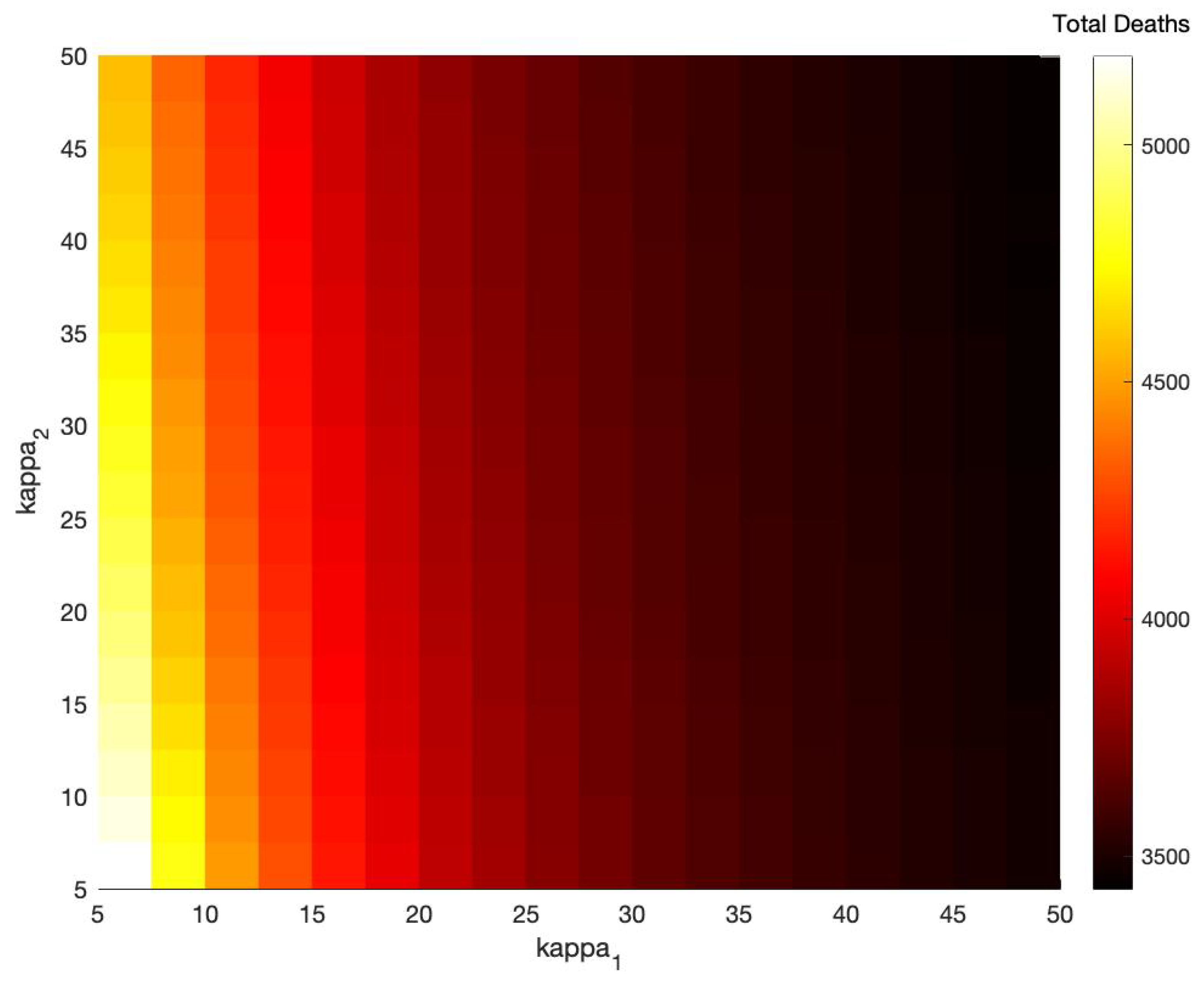
There was a period when the contact tracing infrastructure was overwhelmed by cases, as seen in the plateaus in Figure 4. More contact tracers available to work would have prevented this plateau, but the number of contact tracers available was sufficient to prevent many more cases and deaths from occurring. Increasing either ${\kappa }_1$ or ${\kappa }_2$ would have decreased the number of deaths that occurred, but ${\kappa }_1$ had a stronger effect than ${\kappa }_2$. Overall this work makes a strong contribution to understanding the effects of contact tracing and changes in behavior on disease management.

The results of this paper might be improved if we had more details about the number of contact tracers employed and about the number of individuals being traced through time. More knowledge about the change of behavior during this outbreak would have been useful. One limitation of this model is that we assumed there was no within-hospital transmission, while we know this occurred sometimes.

The practical utility of this model is its use to disease management. One conclusion of our model is that behavior change over the course of an outbreak significantly impacts dynamics and should be considered when formulating models and management responses. It could be interesting to retrospectively analyze other past outbreaks allowing for time-dependent parameters. One could try to connect behavior change with specific information campaigns. Figure 5 shows clearly how a linear decrease in the amount of adequate contact tracing during an outbreak can result in a nonlinear increase in the number of cases and deaths. As a result, our time-dependent modeling approach can be used in future outbreaks to assess the amount of contact tracing that should be conducted in order to limit the total number of cases and deaths.

In the future, we plan to further explore the role of contact tracing in epidemics. To add international spread features, one could consider mobility data [36]. We plan to build a model with a more realistic form to the function f which represents how contact tracing capacity grows in response to an epidemic. We will also explore the role contact tracing plays in outbreaks of other diseases, including diseases with a latent period such as COVID-19. The mechanisms of contact tracing procedures for other diseases might be quite different and require the development of disease-specific models. Optimization techniques (such as optimal control) could be used to design management strategies for contact tracing.