Empirical Convergence Theory of Harmony Search Algorithm for Box-Constrained Discrete Optimization of Convex Function

Abstract

The harmony search (HS) algorithm is an evolutionary computation technique, which was inspired by music improvisation. So far, it has been applied to various scientific and engineering optimization problems including project scheduling, structural design, energy system operation, car lane detection, ecological conservation, model parameter calibration, portfolio management, banking fraud detection, law enforcement, disease spread modeling, cancer detection, astronomical observation, music composition, fine art appreciation, and sudoku puzzle solving. While there are many application-oriented papers, only few papers exist on how HS performs for finding optimal solutions. Thus, this preliminary study proposes a new approach to show how HS converges on an optimal solution under specific conditions. Here, we introduce a distance concept and prove the convergence based on the empirical probability. Moreover, a numerical example is provided to easily explain the theorem.

1. Introduction

In recent years, many researchers have utilized various nature-inspired metaheuristic algorithms for solving scientific and engineering optimization problems. One of the popular algorithms is harmony search (HS), which was inspired by jazz improvisation [1]. As a musician plays a musical note from its memory or randomly, HS generates a value from its memory or randomly. As a new harmony, which is composed of musical notes, is evaluated in each practice and memorized if it is good, a new solution vector, which is composed of values, is evaluated in each iteration and memorized if it performs well. This HS optimization process, which utilizes three basic operations (memory consideration, pitch adjustment, and random selection), continues until it finds an optimal solution vector [2].

When compared with other algorithms, there is a similarity between HS and them [1]. HS is similar to Tabu Search with respect to keeping the past vectors in a memory called harmony memory (HM). In addition, HS can use the adaptative parameters of HMCR (Harmony Memory Consideration Rate) and PAR (Pitch Adjustment Rate), which are similar to Simulated Annealing in varying temperature. Furthermore, both HS and genetic algorithm (GA) manage multiple vectors simultaneously. However, there is also a difference between HS and GA. While HS generates a new vector by considering all the existing vectors, GA generates the new vector by considering only two of the existing vectors (the parents). In addition, HS considers each variable in a vector independently while GA cannot consider in that way because its major operation is crossover, which keeps the gene sequence (multiple variables together).

The HS algorithm has been applied to various optimization problems including project scheduling [3], structural design [4], energy system operation [5], car lane detection [6], ecological conservation [7], model parameter calibration [8], portfolio management [9], banking fraud detection [10], law enforcement [11], disease spread modeling [12], cancer detection [13], astronomical observation [14], music composition [15,16], fine art appreciation [17], and sudoku puzzle solving [18]. Furthermore, there are some application-oriented reviews of HS [19,20,21,22,23,24,25].

While there are many applications proposed so far, only a few studies have been dedicated to the theoretical background of the HS algorithm. Beyer [26] dealt with the expected population variance of several evolutionary algorithms, and Das et al. [27] proposed an approximated variance of the expectation of solution candidates and discussed the exploratory power of the HS algorithm. However, there has been no study discussing the convergence of the HS algorithm while the convergence of other optimization algorithms has been discussed in some studies [28,29,30,31].

As an evolutionary computation algorithm, HS considers an optimization problem:

$$mi{n}_{x\in \mathrm{X}}f\left(x\right),$$

(1)

where

$$\begin{gathered} \mathrm{X}=\{x=\left(x_i\right)\in {\mathrm{R}}^{\mathrm{n}}|l_i<x_i<u_i, i=1,\cdots ,n\}, \\ \mathrm{and}f:R^n\to R. \end{gathered}$$

If all the bounds are infinite, the above problem becomes an unconstrained optimization. However, most practical optimization problems adopt variables having certain prefixed range of values, and, therefore, become box-constrained problems [32].

In this paper, we propose the convergence theory based on the empirical probability for the HS, which is one of box-constrained optimization algorithms. In particular, we consider the convex optimization functions with single and multiple variable cases. For this, we define a discrete sequence to prove convergence using distance. This new approach can be applied to the algorithms, such as HS, which have candidate sets that store the improved solutions in the storage and iteratively update them.

2. Harmony Search Algorithm

2.1. Basic Structure of Harmony Search

The HS algorithm is an optimization method inspired by musical phenomena. This algorithm mimics the musical performing process that occurs when a musician searches for a better harmonic sound, such as jazz improvisation. Jazz improvisation finds a musically pleasing harmony (perfect state) determined by aesthetic standards, just as the optimization process finds a global solution (perfect state) determined by an objective function. While the pitch of each instrument determines its aesthetic quality, the value of each decision/design variable determines its solution quality of the objective function.

In order to optimize a problem using HS, we first define all possible candidate value set called the candidate set (universal set) $\Lambda$. Let us assume that $\Lambda$ includes $K \mathrm{candidate}\mathrm{values}.$ That is, $\Lambda =\left[{\Lambda }_1,\cdots {\Lambda }_n\right]$ and ${\Lambda }_i=\left\{x_i\left(1\right),\cdots ,x_i\left(K_i\right)\right\}.$

Here, the memory storage HM of the HS algorithm can be expressed as in Equation (2). To initialize HM, we randomly choose values from the universal set, and generate vectors as many as HMS (harmony memory size, that is, the number of vectors stored in HM). The value of the objective function is also kept next to each solution vector.

$$\mathrm{HM}=\left[\begin{array}{cccc}{x}_1^1& x_2^1& \cdots & x_n^1\\ x_1^2& x_2^2& \cdots & x_n^2\\ ⋮& \cdots & \cdots & \cdots \\ x_1^{HMS}& x_2^{HMS}& \cdots & x_n^{HMS}\end{array}\hspace{0.17em}|\hspace{0.17em}\begin{array}{c}f(x^1)\\ f(x^2)\\ ⋮\\ f(x^{HMS})\end{array}\right]$$

(2)

Once HM is prepared, the HM is refreshed with better solution vectors iteration by iteration. If a newly generated vector $x_{New}$ is better than the worst vector $x_{\mathit{Worst}}$ stored in the HM in terms of an objective function value, the new vector is swapped with the worst one.

$${\mathrm{HM}}_{\mathrm{New}}=\mathrm{HM}\backslash \left\{x_{Worst}\right\}{{\displaystyle \cup }}^{ }\left\{x_{New}\right\}$$

The value of variable $x_i \left(i=1,2,\cdots ,n\right)$ can be randomly selected from the set of all candidate discrete values ${\Lambda }_i=$$\left\{x_i(1),x_i(2),\dots ,x_i(K_i)\right\}$ with a probability of $P_R$ (random selection rate). Otherwise, the value of $x_i$ can be selected from the set of stored values, named $H{M}_i=\left\{x_i^1, x_i^2,\dots , x_i^{HMS}\right\}$, which is the i^th column of HM, with a probability of $P_M$ (the probability with which the value is selected solely from HM), or, once $x_i\left(k_p^i\right)$ is selected from $H{M}_i$, it can be slightly adjusted by moving it to neighboring values $x_i\left(k_p^i+m\right)$ with a probability of $P_P$ (the probability with which the value is selected solely using pitch adjustment) as follows:

$$x_i^{New}\leftarrow \{\begin{array}{c}{x}_i\left(k_R^i\right)\in {\Lambda }_i, with probability P_R, \\ x_i^h\in H{M}_i, with probability P_M,\\ x_i\left(k_P^i+m\right) \in {\Lambda }_i, with probability P_P,\end{array}$$

(3)

where $=1,\dots ,n;k_R^i,k_P^i\in \left\{1,\dots ,K_i\right\};h\in \left\{1,\dots ,HMS\right\},$ $P_R+P_M+P_P=1\left(100\%\right)$, $0\le P_R,P_M,P_P\le 1,\mathrm{and}m$ is some non-zero integer such that $x_i\left(k_P^i+m\right)\in {\Lambda }_i$. Here, $m$ is a predetermined parameter for adjustment. That is, $m$ = $\pm 1$ or $\pm 2$ or $\pm 3\dots \dots$, etc. For example, if $m$=$\pm 1,$ then we take

$$m=\{\begin{array}{c}1, with probability \frac{1}{2} \\ -1, with probability \frac{1}{2}\end{array}$$

For $P_M$ and $P_P$, we first define HMCR by HMCR $=1-P_R$. Then, after we define PAR, $P_M$ and $P_P$ are defined as $P_M=\mathrm{HMCR}\left(1-\mathrm{PAR}\right)$ and $P_P=\mathrm{HMCR}·\mathrm{PAR}$.

Here, for the pitch adjustment, we first select $x_i^h$ randomly from $H{M}_i$ using a uniform distribution between 0 and 1, i.e., $h=Integer\left(Rand\left(0,1\right)\times HMS+0.5\right).$ Then, we identify $k_P^i,$ which satisfies $x_i^h=x_i\left(k_P^i\right), \mathrm{where}{k}_P^i\in \left\{1,\dots ,K_i\right\}.$ Next, we further tweak $x_i\left(k_P^i\right)$ into $x_i\left(k_P^i+m\right),$ where $x_i\left(k_P^i+m\right)\in {\Lambda }_i.$

This is the basic structure of the HS algorithm [33]. Although there are many structural variants of the HS algorithm [34], most variants basically have the above-mentioned three operations: memory consideration, pitch adjustment, and random selection.

2.2. Solution Formula for Harmony Search without Pitch Adjustment

Let us formulate the solution for the HS algorithm without a pitch adjustment case.

At the first generation, $x_i^1\left(i=1,\dots ,n\right)$ will be chosen with given probabilities as follows:

$$x_i^1=\{\begin{array}{c}{x}_i\left(k\right) from {\Lambda }_i with prob. P_R,\\ x_i^h from H{M}_i^0 with prob. P_M,\end{array}$$

(4)

where $i=1,\dots ,n; k=k_P\in \left\{1,\dots ,K_i\right\}; h\in \left\{1,\dots ,HMS\right\},$ $P_R+P_M=1$ and $H{M}_i^0$ is the initial harmony memory for $x_i$. And let $x_i^g$ be the solution with given probabilities at the $g^{th}$ generation stage, then

$$x_i^g=\{\begin{array}{c}{x}_i\left(k\right) from {\Lambda }_i with prob. P_R,\\ x_i^h from H{M}_i^{g-1} with prob. P_M,\end{array}$$

(5)

where $H{M}_i^{g-1}$ is the newly updated $i^{th}$ column of HM after the ${\left(g-1\right)}^{th}$ generation. At the first generation, $x^1=\left(x_1^1, x_2^1,\dots ,x_n^1\right)$ is obtained by two operations (random selection or memory consideration). If the newly generated vector $x^1$ is better than $x_{\mathit{worst}}^0$ which is the worst vector in $H{M}^0$ in terms of an objective function value, then $x_{\mathit{worst}}^0$ will be replaced with $x^1.$ Otherwise, the worst vector $x_{\mathit{worst}}^0$ will stay in the memory.

The element that we get from this comparison after the first generation will be represented by $x_{\mathit{new}}^1$. That is,

$$x_{\mathit{new}}^1\leftarrow \{\begin{array}{c}{x}^1 if x^1 is better than x_{\mathit{worst}}^0, \\ x_{\mathit{worst}}^0 otherwise.\end{array}$$

(6)

Following a similar procedure, at the $g^{th}$ generation, if $x^g$ is better than $x_{\mathit{worst}}^{g-1}$, which is the worst solution vector in $H{M}^{g-1}$, then ${\mathit{x}}_{\mathit{worst}}^{g-1}$ will be replaced with $x^g.$ Otherwise, the worst element $x_{\mathit{worst}}^{g-1}$ will stay in the memory.

The element that we get from this comparison after the $g^{th}$ generation will be represented by $x_{\mathit{new}}^g$. That is,

$$x_{\mathit{new}}^g\leftarrow \{\begin{array}{c}{x}^g if x^g is better than x_{\mathit{worst}}^{g-1}, \\ x_{\mathit{worst}}^{g-1} otherwise,\end{array}$$

(7)

Using an indicator function, the solution formula for $x_{\mathit{new}}^g$ in Equation (7) can be equivalently represented by:

$$x_{\mathit{new}}^g=x^g·I^g+x_{\mathit{worst}}^{g-1}·\left(1-I^g\right),$$

(8)

where

$$I^g=\{\begin{array}{c} 1 if x^g is better than x_{\mathit{worst}}^{g-1},\\ 0 otherwise.\end{array}$$

(9)

2.3. Solution Formula for Harmony Search with Pitch Adjustment

Next, let us formulate the solution for the HS algorithm with a pitch adjustment case.

At the first generation, $x_i^1\left(i=1,\dots ,n\right)$ will be chosen with given probabilities as follows:

$$x_i^1=\{\begin{array}{c}{x}_i\left(k_R^i\right) from {\Lambda }_i with P_R,\\ x_i^h from H{M}_i^0 with P_M,\\ x_i\left(k_P^i+m\right) from {\Lambda }_i with P_P,\end{array}$$

(10)

where $i=1,\dots ,n; k_R^i,k_P^i\in \left\{1,\dots ,K\right\}; h\in \left\{1,\dots ,HMS\right\},$ $P_R+P_M+P_P=1$ and $H{M}_i^0$ is the initial harmony memory. Then, let $x_i^g$ be the solution with given probabilities at the $g^{th}$ generation stage, in which:

$$x_i^g=\{\begin{array}{c}{x}_i\left(k_R^i\right) from {\Lambda }_i with P_R,\\ x_i^h from H{M}_i^{g-1} with P_M,\\ x_i\left(k_R^i+m\right) from {\Lambda }_i with P_P\end{array}$$

(11)

where $H{M}_i^{g-1}$ is the newly updated $i^{th}$ column of HM after the ${\left(g-1\right)}^{th}$ generation. At the first generation, $x^1=\left(x_1^1, x_2^1,\dots ,x_n^1\right)$ is obtained by three operations (random selection, memory consideration or pitch adjustment). If $x^1$ is better than $x_{\mathit{worst}}^0$ which is the worst one in $H{M}^0$ in terms of an objective function value, then $x_{\mathit{new}}^1=x^1$. Otherwise, $x_{\mathit{new}}^1=x_{\mathit{worst}}^0$. That is,

$$x_{\mathit{new}}^1\leftarrow \{\begin{array}{c}{x}^1 if x^1 is better than x_{\mathit{worst}}^0, \\ x_{\mathit{worst}}^0 otherwise.\end{array}$$

(12)

Therefore, after the first generation, $H{M}^1$ will be updated by substituting $x_{\mathit{worst}}^0$ with $x_{\mathit{new}}^1.$ Then, after the $g^{th}$ generation,

$$x_{\mathit{new}}^g\leftarrow \{\begin{array}{c}{x}^g if x^g performs better than x_{\mathit{worst}}^{g-1}, \\ x_{\mathit{worst}}^{g-1} otherwise,\end{array}$$

(13)

where $x_{\mathit{worst}}^{g-1}$ is the solution vector that performs the worst in the $H{M}^{g-1}$. Therefore, after the $g^{th}$ generation, $H{M}^g$ will be updated by substituting $x_{\mathit{worst}}^0$ with $x_{\mathit{new}}^1.$

Let $x_{\mathit{new}}^g=\widehat{x^g}$. Then, using an indicator function, the solution formula for $\widehat{x^g}$ in Equation (13) can be represented by:

$$\widehat{x^g}=x^g·I^g+x_{\mathit{worst}}^{g-1}·\left(1-I^g\right),$$

(14)

where

$$I^g=\{\begin{array}{c} 1 if x^g performs better than x_{\mathit{worst}}^{g-1},\\ 0 otherwise.\end{array}$$

(15)

3. Empirical Convergence of Harmony Search

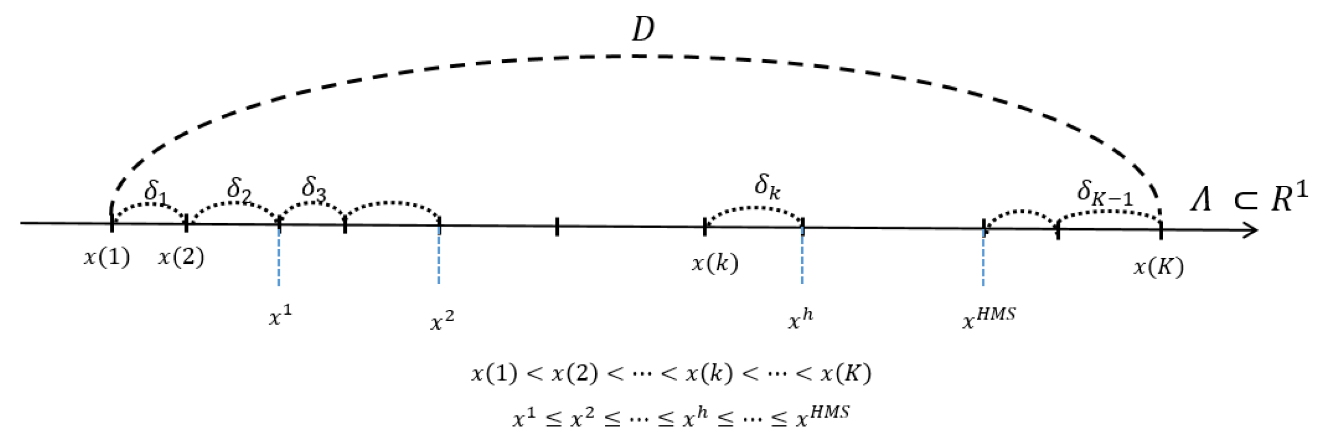
3.1. One Variable Case

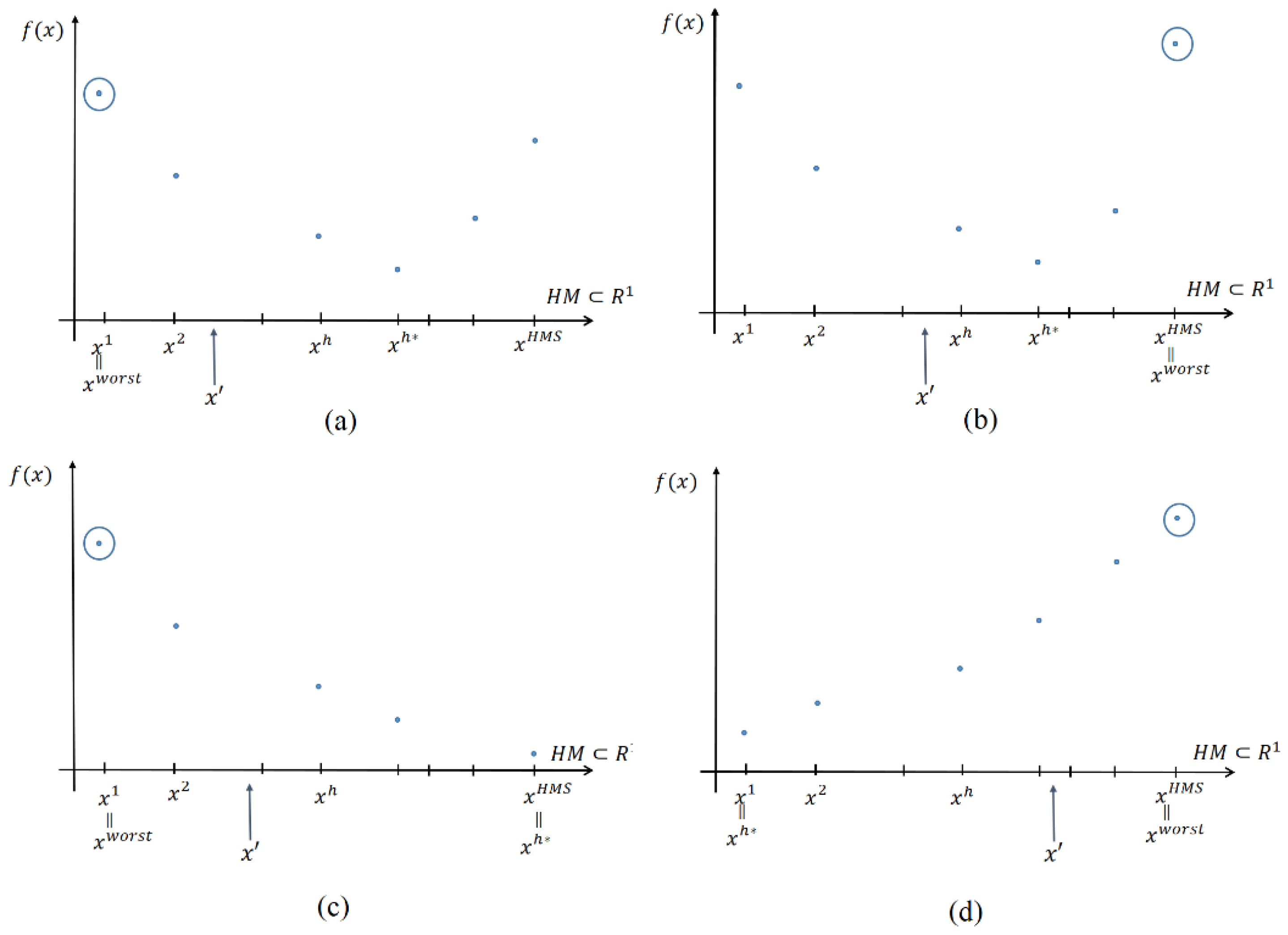
In this section, we discuss the behavior of the solutions in HM. Let us first consider $f\left(x\right)$ is a function of one discrete variable $x$. Without loss of generality, we can assume that $\Lambda =\left\{x\left(k\right)\in R^1|k=1,\cdots ,K\right\}$ satisfies $x\left(1\right)<x\left(2\right)<\cdots <x\left(k\right)<\cdots <x\left(K\right)$ after rearrangement, and we have $K-1$ subintervals that are separated by $x\left(1\right),x\left(2\right),\cdots ,x\left(K\right)$ (See Figure 1). In addition, $HM=\left\{x^h\in R^1|h=1,\cdots ,HMS\right\}$ satisfies $x^1\le x^2\le \cdots \le x^h\le \cdots \le x^{HMS}$ after rearrangement. The $h^{th}$ element of HM at the $g^{th}$ generation will be written as $x^{h,g}$.

Here, let us define the total ranges of the candidate set $\Lambda$ and HM. In addition, we define the distances between neighboring endpoints, which are the lengths of subintervals as follows:

$$D=\left|\Lambda \right|=\left|x\left(K\right)-x\left(1\right)\right|$$

$$D^g=\left|H{M}^g\right|=\left|x_{}^{HMS,g}-x_{}^{1,g}\right|$$

(16)

$${\delta }_k=\left|x\left(k+1\right)-x\left(k\right)\right|, k=1,\cdots , K-1$$

$${\delta }_{h_j}^g=\left|x^{j+1,g}-x^{j,g}\right|, j=1,\cdots , HMS-1\left(\mathrm{at}{g}^{th}\mathrm{generation}\right)$$

(17)

and we define the minimum and maximum value of ${\delta }_k$ as follows:

$${\delta }_m=\underset{1\le k\le K-1}{\min }{\delta }_k \mathrm{and} {\delta }_M=\underset{1\le k\le K-1}{\max }{\delta }_k.$$

(18)

Here, note that we have an important relation as follows:

$$\left(K-1\right){\delta }_m\le D={\displaystyle \sum }_{k=1}^{K-1}{\delta }_k\le \left(K-1\right){\delta }_M.$$

(19)

As we mentioned, we deal with the convex function with discrete variables for its minimum optimal solution. However, note that it can be also applied to the concave function for the maximum optimal solution without loss of generality. If $f\left(x\right)$ has the minimum value at $x^{h*}$, then $x^{h*}$ can be located in four different ways. Figure 2 shows these four different cases. (a) and (b) show the convex objective functions. In this paper, we focus on the convex cases where $x^{h*}$ is located in the middle of the range of HM, which is also applied to the concave cases. However, this theory can be also applied to the monotone increasing/decreasing objective functions such as (c) and (d) as trivial cases, where $x^{h*}$ is located at the right or left end point.

By Equations (5) and (7), the worst element of HM is replaced with a better element as $g$ is increased. Even though not every generation replaces the worst element of HM with a new one, it is true that the worst element of HM is replaced as $g$ is increased. Now, let us consider the case when HM is updated at the $g^{th}$ generation. From Figure 2, we can consider the following properties.

(a)

& (c): Because $x^1=x_{}^{worst},$ the left-end smallest-value point $x_{}^1$ will be replaced by some value except in the case of $x_{}^{’}=x^1.$ Here, note that $x_{}^1\le x_{}^{’}\le x_{}^{HMS}$. The smallest-value element $x_{}^1$ can be newly updated by $x_{}^{’}$ or $x_{}^2$. Consider that we are at the $g^{th}$ generation. Then, the previous $x_{}^1$ is denoted as $x_{}^{1,g-1}$, and the newly updated smallest one from HM will be denoted as $x_{}^{1,g}$. Here,

$$x_{}^{1,g}=\{\begin{array}{c}{x}_{}^{2,g-1} if x_{}^{2,g-1}<x_{}^{’},\\ x_{}^{’} if x_{}^{2,g-1}\ge x_{}^{’}.\end{array}$$

(20)

It is clear that

$$\left|x_{}^{HMS,g}-x_{}^{1,g}\right|\le \left|x_{}^{HMS,g-1}-x_{}^{1,g-1}\right|.$$

(21)

(b)

& (d): Because $x_{}^{HMS}=x_{}^{worst},$ the right end point $x_{}^{HMS}$ will be replaced by some value except in the case of $x_{}^{’}=x^{HMS}.$ $x_{}^{’}$, which shows better performance than $x_{}^{HMS}$. Here, note that $x_{}^1\le x_{}^{’}\le x_{}^{HMS}$. The largest-value element $x_{}^{HMS}$ can be updated by $x_{}^{’}$ or $x_{}^{HMS-1}$. Consider that we are at the $g^{th}$ generation. Then, the previous $x_{}^{HMS}$ is denoted as $x_{}^{HMS,g-1}$, and the newly updated largest one from HM will be denoted as $x_{}^{HMS,g}$. Here,

$$x_{}^{HMS,g}=\{\begin{array}{c}{x}_{}^{\left(HMS-1\right),g-1} if x_{}^{\left(HMS-1\right),g-1}>x_{}^{’},\\ x_{}^{’} if x_{}^{\left(HMS-1\right),g-1}\le x_{}^{’}.\end{array}$$

(22)

It is clear that

$$\left|x_{}^{HMS,g}-x_{}^{1,g}\right|\le \left|x_{}^{HMS,g-1}-x_{}^{1,g-1}\right|.$$

(23)

Now we prove the following theorem.

Theorem 1.

Assume that there exists exactly one solution in the candidate set$\Lambda$for the objective function$f\left(x\right)$. If$D^g=\left|H{M}^g\right|$is the length of HM at the$g^{th}$ generation, then

(i)

$\left\{D^g\right\}$is a monotone decreasing sequence as$g$is increased.

(ii)

Furthermore, the solutions in HM converge.

Proof. 

(i) As we have seen from Equations (21) and (23), we satisfy

$$D^g\le D^{g-1},$$

(24)

which means the sequence $\left\{D^g\right\}$ is a monotone decreasing sequence.

Note that not every generation makes HM updated. Therefore, we need to define a new notation for the generation that updates HM. If the worst element of HM is replaced by a new element $x^{\prime }$ at $g_1^{th}, g_2^{th},\dots$ generation such that

$$D^{g_l}<D^{g_{l-1}},$$

(25)

then $\left\{g_l|l=1,2,3,\dots \right\}$ is the set of generation numbers that update HM when each update reduces $\left|x^{HMS}-x^1\right|$ in HM. It is clear that

$$\left\{g_l\right\}\subset \left\{g\right\},$$

(26)

i.e., $\left\{g_l\right\}$ a subsequence of $\left\{g\right\}.$

Note that, if there are more than one worst solution in HM, then even if HM is updated, it does not satisfy Equation (25). Therefore, the generation number at that time, it is not an element of $\left\{g_l\right\}$.

Now, we consider that either $D^{g_l}>0$ or $D^{g_l}=0$ is true. Equivalently, if either $D^{g_l}\ge {\delta }_m$ or $D^{g_l}=0$ is true, then, in the case of $D^{g_l}>0$, we have $D^{g_l}\ge {\delta }_m$

Furthermore, for the smallest length of subinterval ${\delta }_m,$ it is easily seen that:

$$D^{g_l}\le D^{g_{l-1}}-{\delta }_m.$$

(27)

Here, we need to check the existence of {$g_l$} because we are not sure if HM is steadily updated as $g$ is increased. That is, we are not sure if we can guarantee $x^{*}\left(=argmin f\left(x\right)\right)$ is selected at certain generation. In addition, it is finally guaranteed based on the relation between empirical probability and theoretical probability. That is, if we repeat the generation, it is guaranteed that $x^{*}$ is surely selected at certain generation. Therefore, there exist each generation number $g_l$($l=1,2, \cdots ),$ which updates HM.

Meanwhile, we have the following property:

$$D^{g_1}\le D^{g_1-1}-{\delta }_m\mathrm{and}{D}^{g_2}\le D^{g_2-1}-{\delta }_m.$$

(28)

HM is updated only at $g_l^{th}$ generation ($l=1,2,3,\cdots$). Therefore, $D^{g_1-1}=D^0\mathrm{and}$ $D^{g_2-1}=D^{g_1}$ because $g_1^{th}$ is the first generation which updates HM. Thus, $H{M}^{g_1-1}=H{M}^{g_1-2}=\cdots =H{M}^0$, where $H{M}^0$ is the initial HM. Since $g_2^{th}$ is the second generation that makes HM updated, $H{M}^{g_2-1}=H{M}^{g_2-2}=\cdots =H{M}^{g_1}.$

If we repeat this procedure $l$ times, we get:

$$D^{g_l}\le D^0-l{\delta }_m,$$

(29)

where $D^0=\left|H{M}^0\right|$ is the initial range of HM. Here, {$D^{g_l}$} is a subsequence of {$D^g$}. Here, $D^{g_l}=D^0-l{\delta }_m,$ is unreasonable form practical point of view. Therefore, we assume that $D^{g_l}<D^0-l{\delta }_m$. Since {$D^g$} is decreasing via monotone, {$D^{g_l}$} is decreasing via monotone as well. Furthermore, {$D^g$} is bounded below by 0. For {$D^g$}, note that we have:

$$D^0=\cdots =D^{g_1-1}>D^{g_1}=D^{g_1+1}=\cdots >D^{g_2}=\cdots >D^{g_3}\cdots$$

(30)

Now, let us define ${ϵ}_l$ as follows:

$${ϵ}_l=D^0-l{\delta }_m.$$

(31)

Since ${ϵ}_l>D^{g_l}\ge 0,$ as $l$ increases, ${ϵ}_l$ can be negative, but we consider only the case of ${ϵ}_l>0$. Therefore, let us have ${ϵ}_l>0$ for $l=1,2,3,\cdots ,L$. Since ${ϵ}_l$ ($l=1,2,3,\cdots ,L$) have discrete values, we see that $\{{ϵ}_l$} is a positive decreasing sequence (See Figure 3a). As $g$ is increased, $g_{1,}{g}_2,\dots$ exist empirically. Therefore, every time HM is updated, the sequence ${ϵ}_l$ is decreased. That is, as $l$ increases,

$${ϵ}_1>{ϵ}_2>\cdots >{ϵ}_l>\cdots >{ϵ}_L>0.$$

(32)

Assume that the solutions in HM converge after the $g_t^{th}$ generation. Then,

$$D^0>D^{g_1}>D^{g_2}>\cdots >D^{g_t}=D^{g_{t+1}}=D^{g_{t+2}}=\cdots =D^{g_L}$$

(33)

And it is true that:

$$D^{g_t}<D^0-t{\delta }_m={ϵ}_t,\mathrm{but}{ϵ}_t\mathrm{is}\mathrm{not}\mathrm{very}\mathrm{small},$$

(34)

because ${\delta }_m$ is the minimum length of subintervals. Therefore, we continue the procedure even after the solutions in HM converge until ${ϵ}_l$ is very small but positive. We repeat the generation $s$ more times after the $g_t^{th}$ generation until we satisfy:

$$D^{g_{t+s}}<D^0-\left(t+S\right){\delta }_m={ϵ}_{t+s},\mathrm{and}{ϵ}_{t+s}>0,$$

(35)

$$D^{g_{t+s+1}}<D^0-\left(t+S+1\right){\delta }_m={ϵ}_{t+s+1},\mathrm{but}{ϵ}_{t+s+1}<0,$$

(36)

for some positive integer $s$. However, Equation (36) is not possible because we assume that ${ϵ}_l>0,$ so we stop the procedure after $s$ more generations. Therefore, ${ϵ}_{t+s}={ϵ}_L.$ Here, ${ϵ}_L$ is still a positive constant as in Figure 3b. But,

$${ϵ}_L<{\delta }_m\le {\delta }_{HMS-1}.$$

(37)

Since we have either $D^{g_l}\ge {\delta }_m$ or $D^{g_l}=0$, Equations (35)–(37) guarantee that $D^{g_{t+s}}=D^{g_L}$ is now 0. It means that, at the $g_L^{th}$ generation, it is guaranteed that:

$$x_{}^{1,g_L}=x_{}^{2,g_L}=\cdots =x_{}^{HMS,g_L}.$$

(38)

In fact, Equation (38) has been already satisfied from the $g_t^{th}$ generation, but now the convergence is finally guaranteed by the inequality (34) mathematically. That is, the values in HM are convergent before the $g_L^{th}$ generation. Therefore, we can conclude that there exists some $t<L$ for some positive integers $t \mathrm{and} L$ such that $H{M}^{g_t}$ is convergent.

Therefore, the values in HM converge empirically, which proves the theorem. □

Remark. 

In the general probability theory, for each eventE of the sample spaceS, we definen(E) to be the number of times in the firstn repetitions of the experiment that the eventE occurs. ThenP(E), which is the probability of the eventE, is defined as:

$$P\left(E\right)=P_E=\underset{n\to \infty }{\lim }\frac{n\left(E\right)}{n}.$$

(39)

Here, P(E) is defined as the (limiting) proportion of time that E occurs. It is, thus, the limiting frequency of E.$P\left(E\right)=P_E$is called the “theoretical probability” and$\frac{n\left(E\right)}{n}$is called the “empirical probability.” The empirical probability approaches the theoretical probability as the number of experiments is increased. It means when the repetition number n is small, the event E may not occur. However, if we repeat the experiment many times, i.e., if n is large enough, the ratio between n(E) and n converges$P_E$. It guarantees that the E should occur (even n(E) times) if we repeat the experiment many times. Therefore, even when HM does not include the solution, that minimizes$f\left(x\right)$, if$\Lambda$includes the unique solution, say$x^{*}.$Then it is absolutely selected as we repeat the iteration. That is:

$$P\left[x^{*} is selected\right]=P_R·\underset{g\to \infty }{\lim }\frac{n\left(E\right)}{g}=P_R·\frac{1}{K}$$

(40)

where the event E is the event of selection of$x^{*}$. In addition, Equation (25) guarantees that$x^{*}$should be selected as$g\to \infty$.

Example 1.

Let us consider the situation when the minimum value of the objective function$f\left(x\right)$is at the right end side, as in Figure 2c. Define:

$$\Lambda =\{\frac{k}{10}|k=0,1,2,\cdots ,120\}\mathrm{and}H{M}^0=\left\{0, 2, 3, 3.7, 6, 9, 11\right\}.$$

(41)

Then, as$g$increases, we get$g_1, g_2,\cdots$. As we see from Figure 4, we have$D^0=11,$and

$${\delta }_{h_1}=2, {\delta }_{h_2}=1,{\delta }_{h_3}=0.7, {\delta }_{h_4}=2.3, {\delta }_{h_5}=3, {\delta }_{h_6}=2,\mathrm{and}{\delta }_m=0.7.$$

(42)

Furthermore, we get:

$$D^0=11,D^{g_1}=9, D^{g_2}=8, D^{g_3}=7.3, D^{g_4}=5, D^{g_5}=2, D^{g_6}=0.$$

(43)

Therefore, $t=6$ from Equation (43). However, from ${\delta }_m=0.7,$

$${ϵ}_0=11, {ϵ}_1=10.3,{ϵ}_2=9.6,{ϵ}_3=8.9,{ϵ}_4=8.2,{ϵ}_5=7.5,{ϵ}_6=6.8.$$

(44)

we get ${ϵ}_6=6.8>0$ and it is not a very small number yet. Therefore, we repeat the procedure s more times until we get Equations (35) and (36). It can be easily calculated that $\mathrm{s}=15$. Hence,

$$D_{6+15}<{ϵ}_{6+15}=0.5 < {\delta }_m=0.7$$

(45)

We have either $D^{g_l}\ge {\delta }_m$ or $D^{g_l}=0$ by the definition of $D^{g_l}$. Therefore, Equation (45) guarantees that $D^{g_{21}}=0$. Figure 4 shows the convergence of HM in Example 1. In fact, we already have $D^{g_6}=0$, but it is not proven mathematically yet. Therefore, it is finally shown after 15 more generations as follows.

$$D^{g_6}=D^{g_7}=\cdots =D^{g_{21}}=0$$

(46)

Therefore, there exists a positive integer $t=6\mathrm{that}\mathrm{is}\mathrm{less}\mathrm{than}L=21$ such that the solution in $H{M}^{g_6}$ is convergent. Example 1 shows Theorem 1 is confirmed.

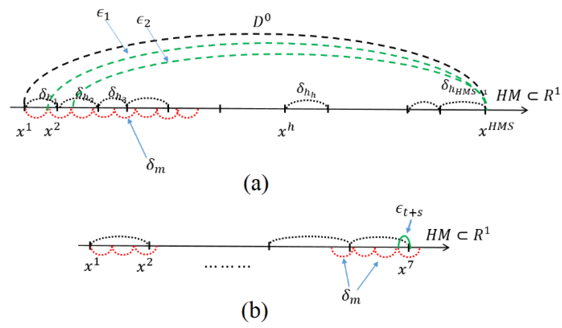
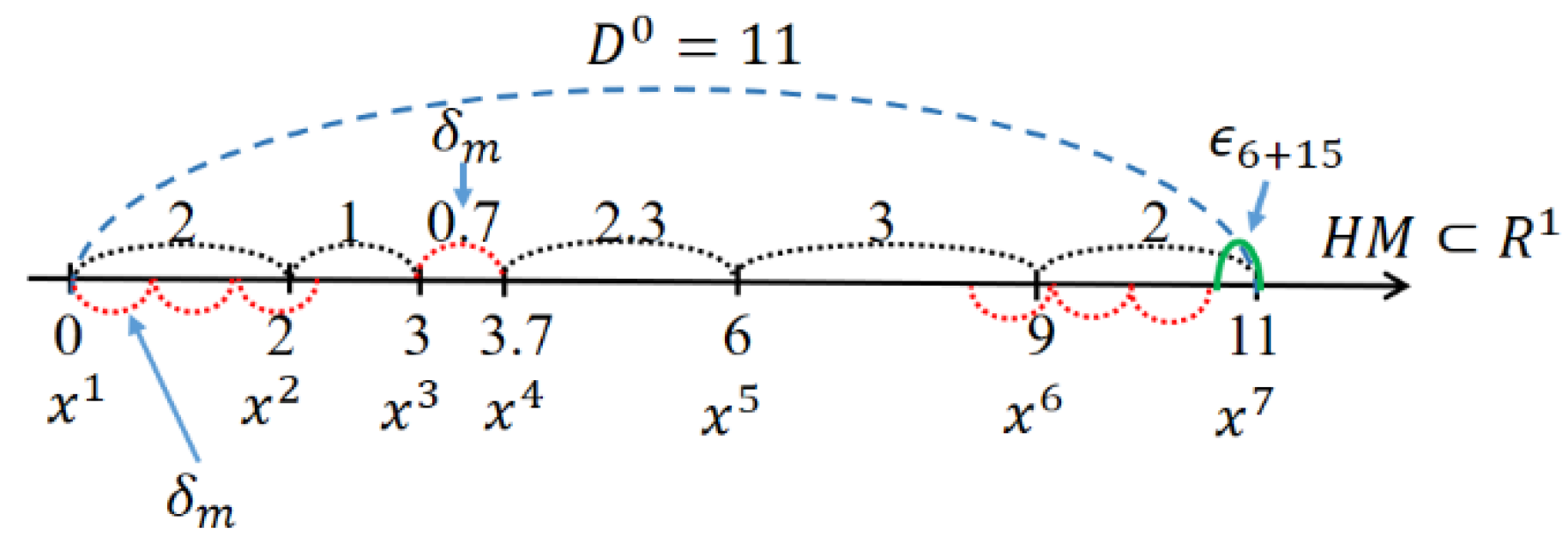
3.2. Multiple Variable Case

Let $f\left(x\right)$ be a function of n variables. Let $x=\left(x_1\left(k\right),\cdots ,x_n\left(k\right)\right)\in R^n$ be a candidate solution from the candidate set $\Lambda .$ Let us consider the norm $\left||·|\right|$ of each solution vector as follows:

$$\left|\left|x\left(k\right)\right|\right|={\left[{{\displaystyle \sum }}_{i=1}^n{x}_i^2\left(k\right)\right]}^{1/2}.$$

(47)

Without loss of generality, we can assume that $\Lambda =\left\{x\left(k\right)\in R^n|k=1,\cdots ,K\right\}$ satisfies $\left|\left|x\left(1\right)\right|\right|<\left|\left|x\left(2\right)\right|\right|<\cdots <\left|\left|x\left(k\right)\right|\right|<\cdots <\left|\left|x\left(K\right)\right|\right|$ after rearrangement, and we have $K-1$ distances between $K$ vectors. The distance between two vectors $x\left(k_1\right)$ and $x\left(k_2\right)$ is defined by:

$$d\left(x\left(k_1\right),x\left(k_2\right)\right)=\left|\left|x\left(k_1\right)-x\left(k_2\right)\right|\right|={\left[{{\displaystyle \sum }}_{i=1}^n{\left(x_i\left(k_1\right)-x_i\left(k_2\right)\right)}^2\right]}^{1/2}.$$

(48)

In addition, $HM=\left\{x^h\in R^n|h=1,\cdots ,HMS\right\}$ satisfies $\left|\left|x^1\right|\right|\le \left|\right|x^2\left|\left|\le \cdots \le \right|\right|x^h\left|\left|\le \cdots \le \left|\right|x^{HMS}\right|\right|$ after rearrangement. The $h^{th}$ vector of HM at the $g^{th}$ generation will be written as $x^{h,g}$.

Here, let us define the total ranges of the candidate set $\Lambda$ and HM. Similarly, without loss of generality, we focus on the minimum case for this optimal solution problem in this section because we can easily apply this theory to the maximum case. In addition, we define the distances between neighboring solution candidate vectors, which are the lengths of subintervals as follows.

$$D=\left|\Lambda \right|=\left|\left|x\left(K\right)-x\left(1\right)\right|\right|$$

$$D^g=\left|H{M}^g\right|=\left|\left|x^{HMS,g}-x^{1,g}\right|\right|$$

(49)

$${\delta }_k=\left|\left|x\left(k+1\right)-x\left(k\right)\right|\right|, k=1,\cdots , K-1$$

$${\delta }_{h_j}=\left|\left|x^{j+1}-x^j\right|\right|, j=1,\cdots , HMS-1$$

(50)

Then we define the minimum and maximum value of ${\delta }_k$ as follows:

$${\delta }_m=\underset{1\le k\le K-1}{\min }{\delta }_k \mathrm{and} {\delta }_M=\underset{1\le k\le K-1}{\max }{\delta }_k.$$

(51)

Here, note that we have an important relation as follows:

$$\left(K-1\right){\delta }_m\le D={\displaystyle \sum }_{k=1}^{K-1}{\delta }_k\le \left(K-1\right){\delta }_M$$

$$HM=\left\{x^h\in R^n|\left|\left|x^1\right|\right|\le \cdots \le \left|\left|x^h\right|\right|\le \cdots \left|\left|x^{HMS}\right|\right|\right\}$$

(i)

If $x^1=x^{worst},$ then $x^1$ will be replaced by some $x\prime ,$ which shows better performance than $x^1$. Here, note that $\left|\left|x^1\right|\right|<\left|\left|x\prime \right|\right|<\left|\left|x^{HMS}\right|\right|.$ Therefore, $x^1,$ which has the smallest norm, will be newly replaced by $x\prime$. Consider that we are at the $g^{th}$ generation, then the previous $x^1$ is denoted as $x^{1,g-1}$. At that point, the newly updated smallest vector from HM will be denoted as $x^{1,g}$. Here,

$$x^{1,g}=\{\begin{array}{c}{x}^{2,g-1} if \left|\left|x^{2,g-1}\right|\right|<\left|\left|x\prime \right|\right|,\\ x\prime o.w.\end{array}$$

(52)

It is clear that

$$\left|\left|x^{HMS,g}-x^{1,g}\right|\right|\le \left|\left|x^{HMS,g-1}-x^{1,g-1}\right|\right|.$$

(53)

(ii)

If $x^{HMS}=x^{\mathit{worst}},$ then $x^{HMS}$ will be replaced by another vector $x\prime ,$ which shows better performance than $x^{HMS}$. Here, note that $\left|\left|x^1\right|\right|<\left|\left|x\prime \right|\right|<\left|\left|x^{HMS}\right|\right|$. Therefore, $x^{HMS},$ which has the largest norm, will be newly replaced by $x\prime$. Consider that we are at the $g^{th}$ generation. Then the previous $x^{HMS}$ is denoted as $x^{HMS,g-1}$. Then, the newly updated largest vector from HM will be denoted as $x^{HMS,g}$. Here,

$$x^{HMS,g}=\{\begin{array}{c}{x}^{\left(HMS-1\right),g-1} if \left|\left|x^{\left(HMS-1\right),g-1}\right|\right|<\left|\left|x\prime \right|\right|,\\ x\prime o.w.\end{array}$$

(54)

It is clear that:

$$\left|\left|x^{HMS,g}-x^{1,g}\right|\right|\le \left|\left|x^{HMS,g-1}-x^{1,g-1}\right|\right|.$$

(55)

Corollary 2. Assume that there exists exactly one solution vector in the candidate set $\Lambda$ for the objective function $f\left(x\right)=f\left(x_1,x_2,\cdots ,x_n\right)$. In addition, if $D^g=\left|H{M}^g\right|=\left|\left|x^{HMS,g}-x^{1,g}\right|\right|$ is the length of HM at the $g^{th}$ generation, then

(i)

$\left\{D^g\right\}$ is a monotone decreasing sequence as $g$ is increased.

(ii)

Furthermore, the values in HM converge.

Proof. 

Based on the notation that are defined in Equations (47)–(51), the proof is clearly done by Theorem 1. □

4. Conclusions

In this communication, we employed the distance concept and proved the convergence of the HS algorithm based on the empirical probability. The solution behavior of HS for one or more discrete variables was discussed and the given theorem was demonstrated with a numerical example.

For the future study, we will expand the theorem to include non-discrete variables, multi-modal functions, and adaptive parameters [35].

References

1. Geem, Z.W.; Kim, J.H.; Loganathan, G.V. A new heuristic optimization algorithm: Harmony search. Simulation 2001, 76, 60–68. [Google Scholar] [CrossRef]
2. Lee, K.S.; Geem, Z.W. A new metaheuristic algorithm for continuous engineering optimization: Harmony search theory and practice. Comput. Methods Appl. Mech. Eng. 2004, 194, 3902–3933. [Google Scholar] [CrossRef]
3. Geem, Z.W. Multiobjective Optimization of Time-Cost Trade-Off Using Harmony Search. J. Constr. Eng. Manag. ASCE 2010, 136, 711–716. [Google Scholar] [CrossRef]
4. Geem, Z.W. Harmony Search Algorithms for Structural Design Optimization; Springer: Berlin, Germany, 2009. [Google Scholar]
5. Nazari-Heris, M.; Mohammadi-Ivatloo, B.; Asadi, S.; Kim, J.-H.; Geem, Z.W. Harmony search algorithm for energy system applications: An updated review and analysis. J. Exp. Theor. Artif. Intell. 2019, 31, 723–749. [Google Scholar] [CrossRef]
6. Moon, Y.Y.; Geem, Z.W.; Han, G.-T. Vanishing point detection for self-driving car using harmony search algorithm. Swarm Evol. Comput. 2018, 41, 111–119. [Google Scholar] [CrossRef]
7. Geem, Z.W. Can Music Supplant Math in Environmental Planning? Leonardo 2015, 48, 147–150. [Google Scholar] [CrossRef]
8. Lee, W.-Y.; Ko, K.-E.; Geem, Z.W.; Sim, K.-B. Method that determining the Hyperparameter of CNN using HS Algorithm. J. Korean Inst. Intell. Syst. 2017, 27, 22–28. [Google Scholar] [CrossRef] [Green Version]
9. Tuo, S.H. A Modified Harmony Search Algorithm for Portfolio Optimization Problems. Econ. Comput. Econ. Cybern. Stud. Res. 2016, 50, 311–326. [Google Scholar]
10. Daliri, S. Using Harmony Search Algorithm in Neural Networks to Improve Fraud Detection in Banking System. Comput. Intell. Neurosci. 2020, 2020, 6503459. [Google Scholar] [CrossRef] [PubMed]
11. Shih, P.-C.; Chiu, C.-Y.; Chou, C.-H. Using Dynamic Adjusting NGHS-ANN for Predicting the Recidivism Rate of Commuted Prisoners. Mathematics 2019, 7, 1187. [Google Scholar] [CrossRef] [Green Version]
12. Fairchild, G.; Hickmann, K.S.; Mniszewski, S.M.; Del Valle, S.Y.; Hyman, J.M. Optimizing human activity patterns using global sensitivity analysis. Comput. Math. Organ Theory 2014, 20, 394–416. [Google Scholar] [CrossRef] [PubMed] [Green Version]
13. Elyasigomari, V.; Lee, D.A.; Screen, H.R.C.; Shaheed, M.H. Development of a two-stage gene selection method that incorporates a novel hybrid approach using the cuckoo optimization algorithm and harmony search for cancer classification. J. Biomed. Inform. 2017, 67, 11–20. [Google Scholar] [CrossRef] [PubMed]
14. Deeg, H.J.; Moutou, C.; Erikson, A.; Csizmadia, S.; Tingley, B.; Barge, P.; Bruntt, H.; Havel, M.; Aigrain, S.; Almenara, J.M.; et al. A transiting giant planet with a temperature between 250 K and 430 K. Nature 2010, 464, 384–387. [Google Scholar] [CrossRef] [PubMed] [Green Version]
15. Geem, Z.W.; Choi, J.Y. Music Composition Using Harmony Search Algorithm. Lect. Notes Comput. Sci. 2007, 4448, 593–600. [Google Scholar]
16. Navarro, M.; Corchado, J.M.; Demazeau, Y. MUSIC-MAS: Modeling a harmonic composition system with virtual organizations to assist novice composers. Expert Syst. Appl. 2016, 57, 345–355. [Google Scholar] [CrossRef]
17. Koenderink, J.; van Doorn, A.; Wagemans, J. Picasso in the mind’s eye of the beholder: Three-dimensional filling-in of ambiguous line drawings. Cognition 2012, 125, 394–412. [Google Scholar] [CrossRef] [PubMed] [Green Version]
18. Geem, Z.W. Harmony Search Algorithm for Solving Sudoku. Lect. Notes Comput. Sci. 2007, 4692, 371–378. [Google Scholar]
19. Geem, Z.W. Music-Inspired Harmony Search Algorithm: Theory and Applications; Springer: New York, NY, USA, 2009. [Google Scholar]
20. Manjarres, D.; Landa-Torres, I.; Gil-Lopez, S.; Del Ser, J.; Bilbao, M.N.; Salcedo-Sanz, S.; Geem, Z.W. A Survey on Applications of the Harmony Search Algorithm. Eng. Appl. Artif. Intell. 2013, 26, 1818–1831. [Google Scholar] [CrossRef]
21. Askarzadeh, A. Solving electrical power system problems by harmony search: A review. Artif. Intell. Rev. 2017, 47, 217–251. [Google Scholar] [CrossRef]
22. Yi, J.; Lu, C.; Li, G. A literature review on latest developments of Harmony Search and its applications to intelligent manufacturing. Math. Biosci. Eng. 2019, 16, 2086–2117. [Google Scholar] [CrossRef]
23. Ala’a, A.; Alsewari, A.A.; Alamri, H.S.; Zamli, K.Z. Comprehensive Review of the Development of the Harmony Search Algorithm and Its Applications. IEEE Access 2019, 7, 14233–14245. [Google Scholar]
24. Alia, M.; Mandava, R. The variants of the harmony search algorithm: An overview. Artif. Intell. Rev. 2011, 36, 49–68. [Google Scholar] [CrossRef]
25. Gao, X.Z.; Govindasamy, V.; Xu, H.; Wang, X.; Zenger, K. Harmony Search Method: Theory and Applications. Comput. Intell. Neurosci. 2015, 2015, 258491. [Google Scholar] [CrossRef] [PubMed] [Green Version]
26. Beyer, H.-G. On the dynamics of EAs without selection. In Foundations of Genetic Algorithms; Banzhaf, W., Reeves, C., Eds.; Morgan Kaufmann: San Francisco, CA, USA, 1999; Volume 5, pp. 5–26. [Google Scholar]
27. Das, S.; Mukhopadhyay, A.; Roy, A.; Abraham, A. Exploratory Power of the Harmony Search Algorithm: Analysis and Im-provements for Global Numerical Optimization. IEEE Trans. Sys. Man Cybern. Part B Cybern. 2001, 41, 89–106. [Google Scholar] [CrossRef]
28. Wu, C.F.J. On the convergence properties of the EM algorithm. Ann. Stat. 1983, 11, 95–103. [Google Scholar] [CrossRef]
29. Bull, A.D. Convergence Rates of Efficient Global Optimization Algorithms. J. Mach. Learn. Res. 2011, 12, 2879–2904. [Google Scholar]
30. Trelea, I.C. The particle swarm optimization algorithm: Convergence analysis and parameter selection. Inf. Process. Lett. 2003, 85, 317–325. [Google Scholar] [CrossRef]
31. Zhang, X.; Zheng, X.; Cheng, R.; Qiu, J.; Jin, Y. A competitive mechanism based multi-objective particle swarm optimizer with fast convergence. Inf. Sci. 2018, 427, 63–76. [Google Scholar] [CrossRef]
32. Facchinei, F.; Júdice, J.; Soares, J. Generating Box-Constrained Optimization Problems. ACM Trans. Math. Softw. 1997, 23, 443–447. [Google Scholar] [CrossRef]
33. Geem, Z.W. Novel derivative of harmony search algorithm for discrete design variables. Appl. Math. Comp. 2008, 199, 223–230. [Google Scholar] [CrossRef]
34. Zhang, T.; Geem, Z.W. Review of Harmony Search with Respect to Algorithm Structure. Swarm Evol. Comput. 2019, 48, 31–43. [Google Scholar] [CrossRef]
35. Almeida, F.; Giménez, D.; López-Espín, J.J.; Pérez-Pérez, M. Parameterized Schemes of Metaheuristics: Basic Ideas and Applications with Genetic Algorithms, Scatter Search, and GRASP. IEEE Trans. Syst. Man Cybern. Syst. 2013, 43, 570–586. [Google Scholar] [CrossRef]
Figure 1. Elements of the candidate set and the subintervals.
Mathematics 09 00545 g001
Figure 2. Candidate solutions and the worst element of one-variable functions.
Mathematics 09 00545 g002
Figure 3. Convergence process when x w o r s t is located at the left end side.
Mathematics 09 00545 g003
Figure 4. Convergence process in Example 1.
Mathematics 09 00545 g004
Publisher’s Note: MDPI stays neutral with regard to jurisdictional claims in published maps and institutional affiliations.