Article

Study on the Intelligent Modeling of the Blade Aerodynamic Force in Compressors Based on Machine Learning

1
Faculty of Science, Beijing University of Technology, Beijing 100124, China
2
School of Energy and Power, Beihang University, Beijing 100191, China
*
Author to whom correspondence should be addressed.
Mathematics 2021, 9(5), 476; https://doi.org/10.3390/math9050476
Submission received: 28 December 2020 / Revised: 22 February 2021 / Accepted: 22 February 2021 / Published: 25 February 2021
(This article belongs to the Special Issue Applications of Mathematical Models in Engineering)

Abstract

:
In order to obtain the aerodynamic loads of the vibrating blades efficiently, the eXterme Gradient Boosting (XGBoost) algorithm in machine learning was adopted to establish a three-dimensional unsteady aerodynamic force reduction model. First, the database for the unsteady aerodynamic response during the blade vibration was acquired through the numerical simulation of flow field. Then the obtained data set was trained by the XGBoost algorithm to set up the intelligent model of unsteady aerodynamic force for the three-dimensional blade. Afterwards, the aerodynamic load could be gained at any spatial location during blade vibration. To evaluate and verify the reliability of the intelligent model for the blade aerodynamic load, the prediction results of the machine learning model were compared with the results of Computation Fluid Dynamics (CFD). The determination coefficient R2 and the Root Mean Square Error (RMSE) were introduced as the model evaluation indicators. The results show that the prediction results based on the machine learning model are in good agreement with the CFD results, and the calculation efficiency is significantly improved. The results also indicate that the aerodynamic intelligent model based on the machine learning method is worthy of further study in evaluating the blade vibration stability.

1. Introduction

With the development of high load and high efficiency in compressors, the centrifugal load and aerodynamic load are endured by the blade due to the strong unsteady flow in the field. Also, the problem of blade vibration has become increasingly prominent. Therefore, the accurate prediction of the internal flow and blade aerodynamic force in the compressor is of great significance for evaluating the reliability of blade vibration in the design stage.
The traditional Computation Fluid Dynamics (CFD) technology can perform a high-fidelity simulation of the linear or non-linear blade vibration in the flow field [1,2,3]. However, it requires high computational expenses for the large-scale calculation. This is not suitable for the rapid evaluation of blade vibration reliability. To overcome the shortcomings of calculation costs [4], the reduced order models of unsteady flow field are proposed here based on the CFD model [5,6,7,8,9,10,11,12]. Proper Orthogonal Decomposition (POD) and Dynamic Mode Decomposition (DMD) are two typical modal decomposition methods, which are based on the flow field feature extraction technology. The complex unsteady flow field is represented with a set of characteristic modes of low-dimensional variables [5,6,7,8,9]. Another kind of reduced-order model based on the system identification technique has been used for the fluid problem [10,11,12]. Simple mathematical mapping was employed to describe the relationship between flow disturbances and aerodynamic characteristics.
In recent years, research on knowledge extraction and data visualization has promoted the exploration of artificial intelligence methods for crossing with fluid mechanics. Machine learning builds a powerful information processing framework with accurate algorithms and generalization capabilities. Efforts have been made for the application of machine learning in fluid mechanics [13,14,15,16,17,18,19,20,21]. The interaction of fluid mechanics and machine learning is summarized by Brunton [13], as well as the development trend of the interdisciplinary approach. It is believed that the application of machine learning can enhance the current fluid mechanics research. Deep Neural Networks (DNN) were stated to play a key role on modeling complex flow by Kutz [14]. A reduction model by DNN was designed based on the data of Direct Numerical Simulation (DNS) by Zhang [15]. The results show that DNN can predict the anisotropic Reynolds stress effectively. Chen [16] proposed the use of a deep Convolutional Neural Network (CNN) to extract flow information, and established a composite network to solve the problem of input with different variables. The hybrid deep neural network framework was used by Han [17] to directly capture the characteristics of unsteady flow in the field. The field predicted by DNN was in agreement with the result calculated by CFD solver. Hasegawa [18] constructed a reduced-order model combined with a CNN auto encoder and Long Short-Term Memory network (LSTM). The model proved to be able to predict the unsteady flow of bluff bodies. Also, the multi-core neural network was adopted by Kou [19] to achieve the correction from the low-order model to the high-fidelity results. A model was constructed with a combination of the Adaptive Simulated Annealing algorithm (ASA) and Recursive Radial Basis Function neural network (RRBF) for the cascade by Hu [20]. It was proven that the ASA-RRBF model has a higher accuracy than the single RRBF model.
The data-driven optimization of machine learning and the application of regression technology can map a high-dimensional flow field to a low-dimensional space, which can effectively solve the high-dimensional nonlinear problems. The ability of machine learning could simplify the treatment of the exploration and visualization of the high-dimensional database, which can greatly improve performance optimization and reduce the convergence cost [13]. The intelligent method provides a useful technology to extract relevant information, which promotes a rapid development of flow dynamics. The constructed reduced-order aerodynamic force model based on the machine learning can predict the unsteady aerodynamic force of the blade with a reasonable accuracy and a low computation cost [21].
Note that the current applications of artificial intelligence method in the fluids are mostly focused on the modeling of flow characteristics, while the modeling of blade aerodynamic force in vibration rarely involves the intelligence method. For this paper, the XGBoost algorithm was applied for the first time to the aerodynamic modeling of an actual compressor blade. A reduced-order intelligent model of the three-dimensional unsteady aerodynamic force of the blade was established for consideration of machine learning and CFD. By learning a small amount of CFD sample data, the trained low-dimensional XGBoost model could effectively capture the characteristics of the unsteady flow. The aerodynamic load of the compressor blade during the vibration process can be obtained by the intelligence model through the input and output mathematical mapping. Compared with the deep learning, the XGBoost model is suitable for data with a small number of variables. It has the advantages of model interpretability and invariance of input data. Also, it is convenient for parameter adjustment to achieve default predictions through automatic iteration. Under the premise of ensuring the accuracy, this reduced-order model presented can greatly reduce the calculation costs.

2. Description of the Machine Learning Algorithm

The eXtreme Gradient Boosting algorithm is an integrated machine learning algorithm based on a decision tree, which is in the foundation of gradient boosting framework. It is proposed to build an efficient and flexible algorithm by Chen [22] according to the second-order information [23]. This algorithm is a scalable machine learning system in the lifting method, which is integrated by multiple regression trees to form a strong classifier. The problem of overfitting in tree model can be effectively avoided [24]. After parallelization, it is more than one order of magnitude faster than similar algorithms under the same conditions [25]. The excellent performance in high-dimensional data analysis shows a strong ability in modeling the complex process [26]. Because of its high performance and low requirement, XGBoost has been widely used in disease prediction, credit debt default risk prediction, driving evaluation, route planning and so on [27,28,29,30].
The principle of its algorithm is to update iteratively the parameters of the previous classifier to reduce the gradient of the loss function and generate a new classifier [31]. By reducing the error of prediction through several regression trees, the regression tree group is guaranteed to have the maximum generalization ability. The regular term is added to the loss function of the model. Then the second-order Taylor expansion of the loss function is solved to determine the split node on the basis of the minimum loss function. The second-order derivative information and the addition of regularization method have improved the performance of generalization and calculation [32]. The structure of the XGBoost algorithm is indicated in Figure 1.
The given sample data set is:
η = { ( x i _ C F D , y i _ C F D ) } ( i = 1 , 2 , , n , x i _ C F D R m , y i _ C F D R )
where x i _ C F D represents the i-th feature value of the sample data, y i _ C F D represents the experiment value of the i-th label of the sample data and x i Pr e represents the predicted value of the i-th label of the model. Define the loss functions of y i _ C F D and y i _ Pr e :
l ( y i _ C F D , y i _ Pr e ) = ( y i _ C F D y i _ Pr e ) 2
Where y i _ Pr e is the prediction in the integration model of the XGBoost system, which uses the sum of the predicted value of each tree (the total number of trees is K) for the sample. Assuming that the tree model to be trained in the k-th iteration is f k ( x ) , the prediction function was defined as follows:
y i _ Pr e = k = 1 K f k ( x i ) , f k Γ Γ = f ( x ) = ω q ( x ) ( q : R m T , ω R T ) .
As Γ is the space of Classification and Regression Trees (CART) numbers, q represents the score of the structure of each tree mapping each sample to the corresponding leaf node; ω q ( x ) represents the set of scores for all leaf nodes of tree q. The optimized parameter in the XGBoost algorithm is defined as the function of f ( x ) . While a tree is added into the model each time, the loss of the objective function was expected to be decreased. The iteration functions could then be expressed as:
y i _ Pr e ( 0 ) = 0 y i _ Pr e ( 1 ) = f 1 ( x i ) = y i _ Pr e ( 0 ) + f 1 ( x i ) y i _ Pr e ( 2 ) = f 1 ( x i ) + f 2 ( x i ) = y i _ Pr e ( 1 ) + f 2 ( x i ) y i _ Pr e ( t ) = k = 1 t f k ( x i ) = y i _ Pr e ( t 1 ) + f t ( x i ) .
The objective function could then be expressed as:
o b j = i = 1 n l ( y i _ C F D , y i _ Pr e ) + i = 1 K Ω ( f i ) Ω ( f ) = γ T + 1 2 λ ω 2 ,
where i = 1 K Ω ( f i ) indicates the regularization term of the loss function, which is the sum of the complexity of all K trees. The number of leaf nodes T is limited with a penalty term Ω ( f i ) so as to prevent overfitting. ω represents the set of scores for all the leaf nodes of each tree, while γ and λ represent the coefficients. In order to solve the optimal objective function, the second-order Taylor expansion of the t-th tree f t ( x i ) in Equation (4) is performed with bringing into the objective function. As the loss function l ( y i _ C F D , y i _ Pr e ( t 1 ) ) is a constant, it can be ignored. And the leaf nodes of all trees can be regrouped. Then the node number and leaf weights are used to optimize the regularization term of the loss function. All samples x i of leaf nodes are divided into a sample set, denoted as I j = { i | q ( x i ) = j } . The objective function could be rewritten as:
o b j = i = 1 n [ l ( y i _ C F D , y i _ Pr e ( t 1 ) ) + g i f t ( x i ) + 1 2 h i f t 2 ( x i ) ] + Ω ( f t ) + c o n s tan t i = 1 n [ g i f t ( x i ) + 1 2 h i f t 2 ( x i ) ] + Ω ( f t ) = i = 1 n [ g i f t ( x i ) + 1 2 h i f t 2 ( x i ) ] + γ T + 1 2 λ j = 1 T ω j 2 = i = 1 n [ g i ω q ( x i ) + 1 2 h i i ω q 2 ( x i ) ] + γ T + 1 2 λ j = 1 T ω j 2 = j = 1 T [ ( i I j g i ) ω j + 1 2 ( i I j h i + λ ) ω j 2 ] + γ T = j = 1 T [ G j ω j + 1 2 ( H j + λ ) ω j 2 ] + γ T ,
where g i = l ( y i _ C F D , y i _ Pr e ( t 1 ) ) y i _ Pr e ( t 1 ) , h i = 2 l ( y i _ C F D , y i _ Pr e ( t 1 ) ) ( y i _ Pr e ( t 1 ) ) 2 , G j = i I j g i , H j = i I j h i , f ( t ) = ω q ( x ) , ω R T q : R d { 1 , 2 , , T } .
The smaller the value of the objective function is, the smaller the prediction error is, with a better generalization ability and robustness of the model. By using the highest value formula of the quadratic function, the weight ω j * of each leaf node could be obtained. The optimal objective function can then be expressed as:
ω j * = G j H i + λ , o b j = 1 2 j = 1 T G j 2 H i + λ + γ T .
The modeling advantage of in XGBoost method can be concluded to the adjunction of regularization items displayed in the objective function. The regularization items are related to the number and the value of leaf nodes in the tree. In addition, the sparse value of the training data in the XGBoost algorithm should be noted. The default direction of the branch is specified for missing values, which greatly improves the efficiency of the algorithm [33]. As an advanced machine learning method developed in recent years, this method has a good performance in processing high-dimensional data with the reduction of the overfitting.

3. Methodology of Aerodynamic Intelligent Model

3.1. Data Collection for Machine Learning

The high accuracy data is the key to establishing an accurate unsteady aerodynamic model of blade in compressor. The training process of the XGBoost model in this paper was mainly driven by the database obtained from the CFD fluid-structure coupling computation. The research object was a 1.5 stage axial compressor, including struts, inlet guide vanes, first stage rotor and stator. Detailed introductions for the rig are presented in Zhang [34].
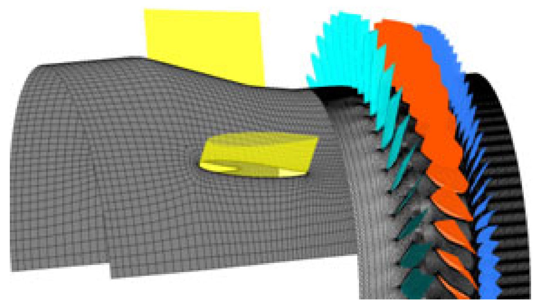
The unsteady flow field in the compressor was solved by using the numerical solution of 3-D Navier-Stokes equations adopted in software ANSYS Package. The spatial discretization of the flow governing equations was employed on an upwind scheme, and a second-order backward differencing was integrated for the time-accurate solution [35]. Boundary conditions imposed on the inlet consist of total pressure and total temperature. A specified average static pressure was implemented at the exit boundary. Smooth, adiabatic and no-slip wall boundary conditions were applied for the flow field solution [36]. While considering the fluid-structure interaction, the blade vibration was computed under the response to the flow. The detail simulation process of the compressor is described in reference [34]. The structural equations for mechanical blade were solved by the finite element method. Within each time step, the flow equations and the structural equations were solved simultaneously, exchanging information on the fluid-structure interface. This procedure was repeated until the flow and displacements were converged, before proceeding to the next time step. The numerical model of the 1.5-stage turbocompressor is shown in Figure 2.
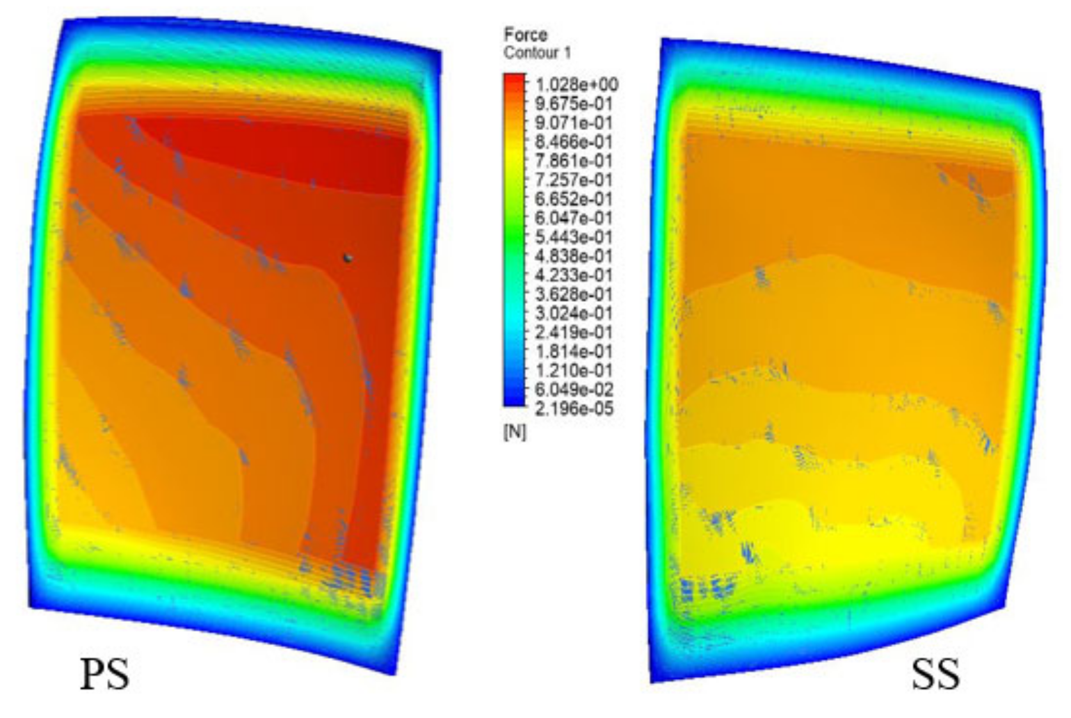
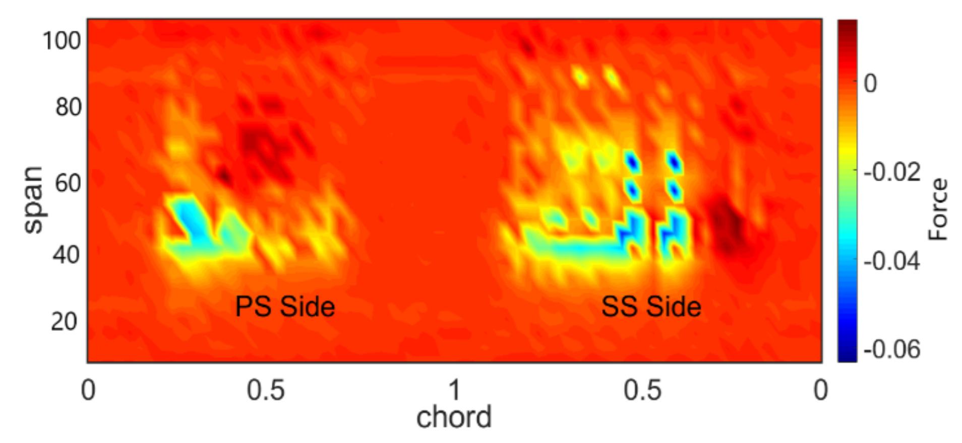
After the convergence of the simulation, the results computed by the commercial CFD software were used for the current data learning, including the spatial unsteady flow data and aerodynamic force on blade surface in time domains. The snapshot data of the unsteady flow was captured at each time step, including pressure and aerodynamic force of the blades at modal coordinates. The data set for training/testing was composed with five variables, such as Cartesian coordinates, pressure and aerodynamic force. The three-dimensional coordinate (X, Y, Z) of the structure space was taken as an input, and the aerodynamic force was taken as an output to form the sample data S = (X, Y, Z, Force). The flow snapshot data extracted from CFD was arranged in time series as a sequence { S 1 , S 2 , S 3 , , S N } , where S i = { X i j , Y i j , Z i j , F o r c e i j } , i = 1 , 2 , , N , j = 1 , 2 , , n . The distribution of the aerodynamic force on the blade surface is shown in Figure 3, which was extracted in the CFD fluid-structure coupling simulation at a single time. It can be seen that the distribution of aerodynamic force was not uniform on both the pressure side (PS) and suction side (SS). Because of the unsteady flow in the field, the aerodynamic force that acted on the blade appears in a non-linear state, which resulted in the vibration blade indicating complex dynamic behaviors.

3.2. Procedure of Aerodynamic Modeling Based on the XGBoost Algorithm

In this part, the methodology of aerodynamic modeling based on XGBoost algorithm is introduced in detail. The procedure can be concluded as follows.
Step 1: Data preprocessing.
After the data collection from CFD, the features of acquired data may have different magnitudes. When the gradient is updated, it may oscillate back and forth, and take a long time to reach the local optimal value or the global optimal value. In order to improve the training efficiency and avoid the numerical error caused by the size difference of the features, the data were handled in normalization. This ensured that the same dimension was achieved for different features, so that the descent of gradient could be a quick convergence. The normalized function form used in this article is shown as follows:
X = x k x min x max x min .
In machine learning algorithms, feature engineering is an important step in the process of modeling. The original data were transformed into the training data with feature engineering, providing the training model with a better robustness and generalization ability. This paper provides three characteristics of index, distance and average value of three-dimensional coordinates based on data information.
Step 2: Training set construction.
The training set was used to estimate the parameters in the intelligent model. As a result, the accuracy and efficiency of the model were determined by the selection of the training set. In order to optimize the effect of the model, the dichotomy process was adopted to partition the training set. That is to say for N samples, each segment was divided into the length of [ C / 2 ] , where C = [ N ] , [ N / 2 ] , [ N / 2 2 ] , , 2 . Then take a representative data set from each segment to form a training set. Taking into account of the accuracy and running time in calculation, two snapshots as { S 1 , S [ N / 2 ] } were selected to form the training set to train the model in this paper.
Step 3: Training process.
The training set after data preprocessing was substituted into the initial XGBoost model established for training. The effect of prediction by the model was evaluated by the comparison to the [ N / 2 ] + 1 snapshot data, which were selected as the test set. The establishment of the model required the setting of hyper-parameters. The hyper-parameters used in this article were defined as: Max-depth (the maximum depth of the tree), Learning-rate (the learning rate), n-estimators (the number of sub-models) and objective (the given loss function). The hyper-parameters for the initialization model are given in Table 1.
Step 4: Parameter Adjustment.
The adjustment of the hyper-parameters in the XGBoost model played a key role in affecting the training performance of the XGBoost algorithm. So, the GridSearchCV function was employed to adjust the parameters of the XGBoost model. The hyper-parameters after seeking are shown in Table 2.
Step 5: Evaluation Criteria.
The indicators as the coefficient of determination R2 and the root mean square error (RMSE) were introduced to evaluate the accuracy of the established XGBoost model. The fitness of the prediction to the observation can be represented by the coefficient of determination R2, which was defined as the ratio of the regression sum of squares to the total sum of squares. This coefficient is often used to evaluate the merits and demerits of a regression model. If the coefficient of determination R2 is calculated to be close to 1, it indicates that the regression model is effective. RMSE is the square root of the ratio, which is the square sum of the errors of prediction values to the number of observations. The optimal parameters of the model and the optimal prediction results were obtained through model training
R 2 = 1 i ( C F D i P r e i ) 2 i ( C F D i C F D i ¯ ) 2 ,
R M S E = i = 1 n ( C F D i P r e i ) 2 n u m ,
where C F D i represents the i-th label in the sample data which is captured from CFD simulation, C F D i ¯ represents the average value of the label in the sample set, and P r e i represents the predicted value of the i-th label in the XGBoost model. And prediction error is defined as: e r r o r = P r e C F D , which is the difference between the prediction of the XGBoost model and the CFD result. The whole procedure of aerodynamic modeling based on the XGBoost algorithm is shown in Figure 4.

4. Modeling of Blade Aerodynamic Pressure Based on Machine Learning

In this section, the intelligent modeling is first performed for the three-dimensional unsteady pressure of the blade during the vibration process. Also, the effectiveness and accuracy of the model are evaluated based on the XGBoost algorithm. The three-dimension coordinate (X, Y, Z) of the state space in blade vibration was taken as the input, and the pressure data was taken as the output to form sample data S = (X, Y, Z, Pressure). According to the procedure of aerodynamic modeling described above, the gradient descent method was used to find the optimal solution. After the dimensionless processing on pressure data, the training set was collected to train the XGBoost model. Also, the test set was brought into the trained optimal prediction model for comparison. Finally, the prediction on the blade aerodynamic pressure was obtained with the XGBoost model established.
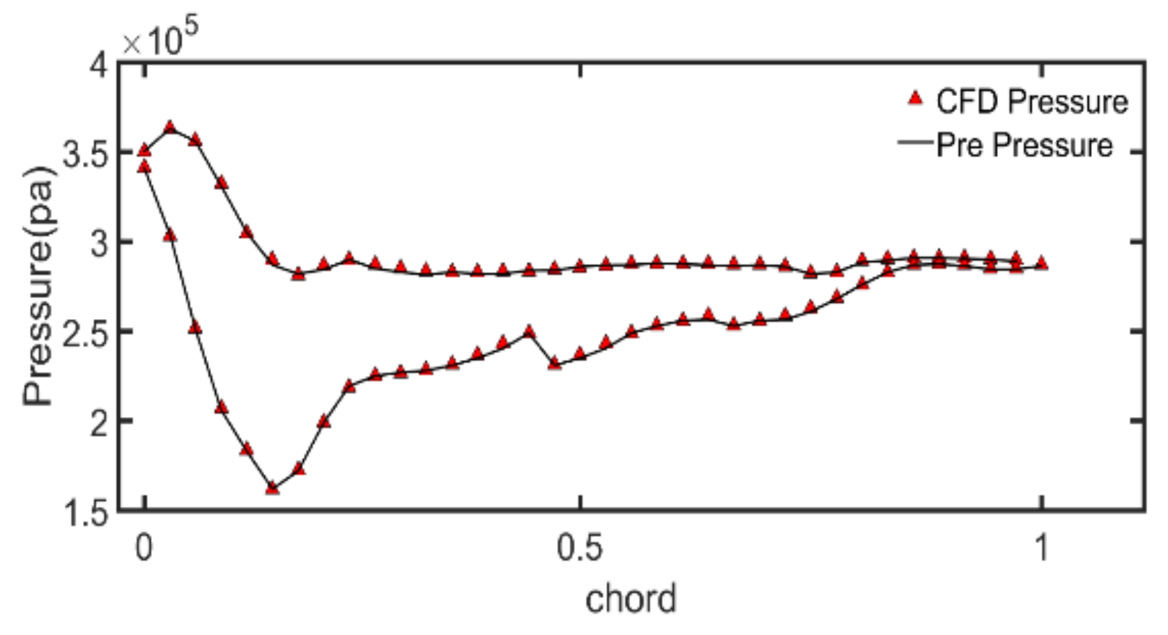
The prediction results of the aerodynamic pressure of blade are shown in Figure 5 at a certain time. The predicted values of pressure in the XGBoost model were compared with the data in CFD simulation at 80% of the blade span. It can be seen that the curves predicted are in good accordance with each other, indicating the accuracy of the XGBoost model.
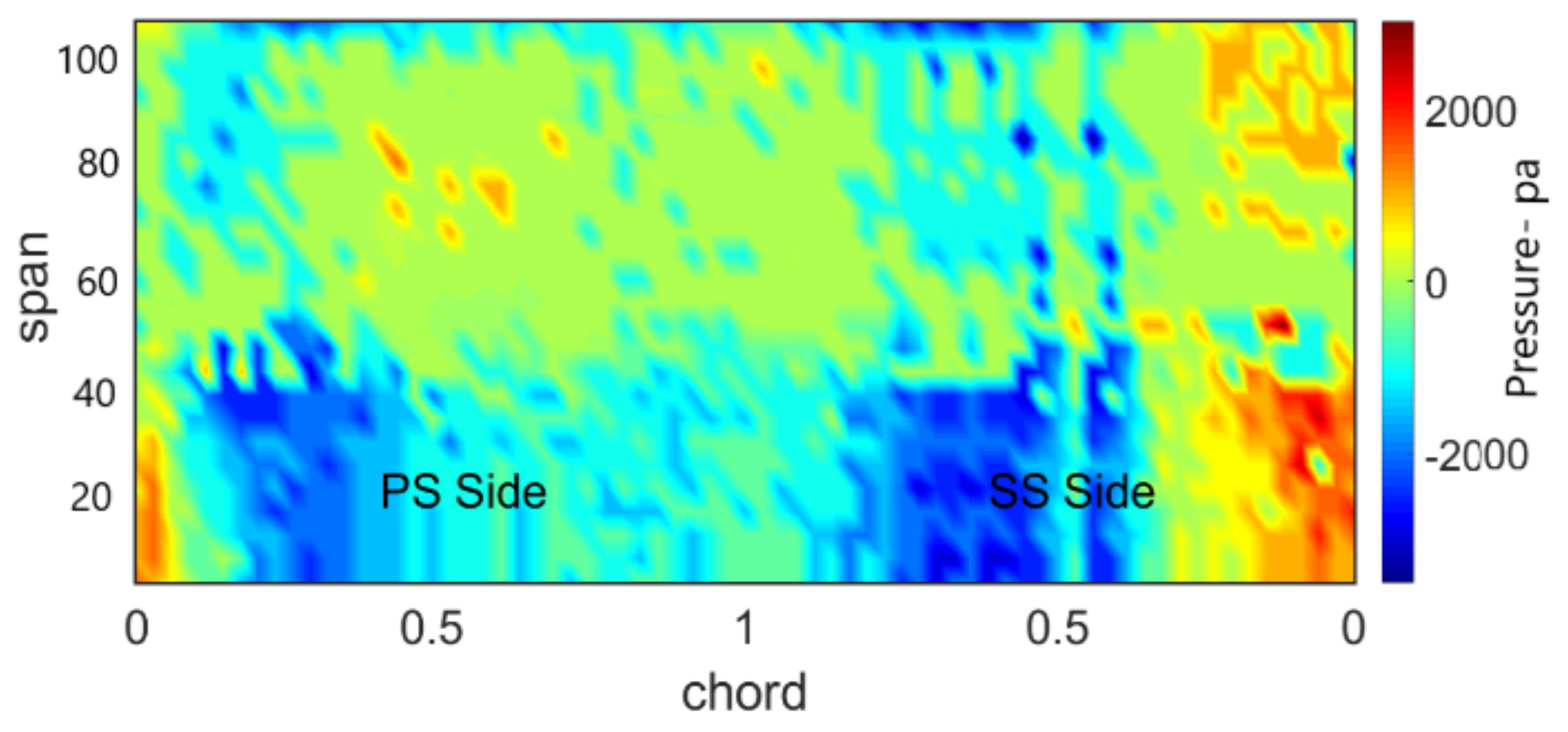
We unfolded the three-dimensional compressor blade along the leading edge, and displayed the pressure surface (PS Side) and suction surface (SS Side) of the compressor blade on the same coordinate plane. The pressure contour predicted by the XGBoost model is exhibited in Figure 6, as well as the result simulated by CFD. The two contours look almost the same, but there are still errors located under 40% of span, which are revealed in Figure 7. In addition, under the program running with 0.3 s, the coefficient of determination R2 was computed to be 0.99947. The RMSE was obtained as 1012.4 by the model, which is approximately a 0.3% error rate to the average pressure of the blade. Compared with CFD simulation data, the three-dimensional aerodynamic pressure model of the blade based on the XGBoost intelligent method reflects a good accuracy and efficiency. The current study demonstrates that it is sufficient to predict the blade aerodynamic force by capturing the characteristic of flow based on the machine learning method.

5. Modeling of Blade Aerodynamic Force Based on Machine Learning

Under the verification for the effectiveness of the intelligent modeling method, the XGBoost algorithm was then used to model the unsteady aerodynamic force for the three-dimensional blade in this section. The aerodynamic force on the blade surface was obtained based on the integral of the pressure over the mesh grid area in CFD. Because of the micro size of grid at the blade edge, the value of force at the blade edge was much smaller. In order to restore the distribution of force on the blade, the process of dimensionless was performed for the aerodynamic force Df on the blade surface
D f = F S ¯ × P ,
where F is the aerodynamic force data on the blade surface in CFD, S ¯ is the average area of the blade surface mesh and P equals the standard atmospheric pressure. Next, the distribution of aerodynamic force on the blade surface was predicted by the XGBoost model at any position during the vibration process.
The predicted values of aerodynamic force in the XGBoost model were chosen here to compare with the data in CFD simulation at 3%, 80% and 90% of the blade span, respectively, as shown in Figure 8. It can be seen that the aerodynamic force of the blade increases sharply from the leading edge, and decreases at the trailing edge. It was found that the values of aerodynamic force appear to have significant differences along the variation of the blade span. The aerodynamic forced distributed along the direction of the blade spanwise presents a nonlinear characteristic.
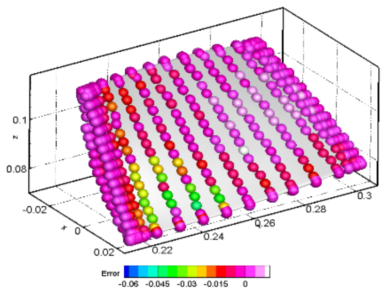
This appearance can also be observed at the distribution of force at the three-dimension surface of the blade. The 3D plots are adopted here to show the distribution of aerodynamic force at a blade modal location. As indicated from Figure 9, it can be seen that the distribution of the aerodynamic force predicted by the XGBoost model is accordant with the CFD data on the pressure surface of the blade. The load of blade is mainly concentrated in the middle part of the blade, corresponding to the region of high aerodynamic force. Because of the non-linear feature, the unsteady force is not easy to express. According to the errors displayed in Figure 10, the nodes of aerodynamic force modeling by XGBoost method show good agreement with the CFD data. Although the existence of error was discovered at certain points, the effectiveness of the aerodynamic force model is still verified through the comparison.
The dimensionless aerodynamic force contour predicted by the XGBoost model is expressed in Figure 11, along with the contour simulated by CFD. The two aerodynamic clouds coincide exactly with each other. Also, the errors inevitably appear in the comparison of XGBoost model with CFD, as indicated in Figure 12. But it can be seen that the errors emerge mostly in the region with a large gradient. The values of error oscillate around 0 with the maximum value as 0.06, which is relatively small in contrast to the dimensionless aerodynamic force of the blade. At the running of program with 0.23 s, the coefficient of determination R2 of the XGBoost model was computed to be 0.99998, which is very close to 1. Also, the RMSE was obtained as 0.005846 by the model, which is approximately a 0.1% error to the average dimensionless aerodynamic force of the blade. With the comparison to the CFD simulation data, this shows a good accuracy and reliability of predicting the aerodynamic force by the three-dimension aerodynamic force model of the blade based on the XGBoost intelligent method.
To check the generalization ability and robustness of the XGBoost model, snapshot data sets with the blade vibration at different times were used as the testing set. The trained XGBoost model was also used to predict the aerodynamic force of each snapshot data in the testing set. The results of prediction are revealed in Figure 13, as represented by the coefficient of determination R2 and RMSE for different testing data. For the trained aerodynamic force XGBoost model, the prediction accuracy also shows a slight discrepancy compared to different positions of blade vibration. The maximum coefficient of determination R2 of the prediction model is 0.99999, with the minimum value as 0.99987. The maximum RMSE value is 0.01852, with the minimum value to be 0.00519. The coefficients of determination R2 are all above 0.9998, and the RMSE values are all less than 0.0186. This means that the XGBoost model reflects a good generalization ability with high robustness. From all analysis above, it can be concluded that the three-dimension aerodynamic model based on the XGBoost algorithm can accurately predict the aerodynamic force of the blade on the basis of any spatial position in the blade vibration process.

6. Discussion

With the assistance of CFD technology, the unsteady flow field simulation of the compressor is considered as a full-order solution to the system. Although the data obtained is regarded as being accurate, it is not convenient for the rapid qualitative analysis of the system with a high time cost and low efficiency [4]. With the simple control equation of the reduced-order model, the data can significantly reduce computation expenses and improve calculation efficiency [10]. The mathematical mapping between the input and output can be set up by solving the complex Navier-Stokes equations once for training. Then the fluid-structure coupled solution in the CFD solver can be replaced by the intelligent model.
Recently there has been research conducted on the aerodynamic reduction modeling of wings by artificial intelligent methods. But there are considerable differences between blades and wings. Compared with isolated wings, there is an obvious unsteady aerodynamic interference effect in the blade row [36]. Therefore, the aeroelastic analysis of blades is different from the traditional vibration analysis of wings in outflow. Since the internal flow is a very complex full three-dimensional unsteady viscous flow field, the aerodynamic interference between the blades is very prominent. It is impossible to use theory to predict the unsteady aerodynamic force of vibrating blades with so many parameters [37]. In nonlinear dynamic analysis, it is assumed that the blade is flat with no thickness, reducing the real three dimensions to two dimensions. However, an efficient and accurate aerodynamic model of the three-dimension blade is the basis for the analysis of the nonlinear dynamic system. The vibration modeling of the actual three-dimensional blades was rarely used in the previous research.
In this paper, the XGBoost algorithm of machine learning was used to establish a reduced-order model of the unsteady aerodynamic force for a vibrating blade. By learning from the high-fidelity sample data, the aerodynamic distribution of a three-dimensional blade could be quickly predicted accurately at any spatial position of the blade during the vibration process. This provides a basis for the further nonlinear dynamic analysis of the blade. But how to incorporate this into the nonlinear dynamics equations with an appropriate format remains a question. It is also worth conducting further integration with fluid mechanics to evaluate the blade vibration stability.

7. Conclusions

The internal field of the compressor is essentially a three-dimensional unsteady flow. The flow around the blade is very complex. In order to achieve an unsteady aerodynamic load on the blade, a reduced-order intelligent model of the three-dimensional blade in compressor was established in this paper based on a machine learning algorithm for the first time. The main conclusions are as follows:
(1)
With the combination of the intelligent algorithm in machine learning and CFD technology, the modeling for the aerodynamic force can be performed for a three-dimensional blade of compressor in vibration. Also, the procedure for aerodynamic modeling based on the XGBoost algorithm was established, which is described as data collection, data preprocessing, training set construction, model training and parameter adjustment.
(2)
The high-fidelity data for model training can be set up by solving the complex Navier-Stokes equations once for the flow field. Then the information of the unsteady flow can be effectively captured based on the XGBoost model training for the mathematical mapping between the input and output. The rapid identification was achieved for the three-dimensional aerodynamic force on the blade, which improves the efficiency of calculation.
(3)
Based on the data of blade vibration in CFD simulation, an intelligent model based on the XGBoost algorithm was established for the prediction of the three-dimensional unsteady aerodynamic pressure and force. With the comparison to the CFD data, it showed a good accuracy and reliability on the prediction in the XGBoost intelligent method. The distribution of an unsteady aerodynamic load on the blade can be accurately predicted on the basis of any spatial position in the blade vibration process. It provides a new perspective for the analysis of blade nonlinear dynamics. The aerodynamic intelligent model based on the machine learning is worthy of further integration with fluid mechanics for evaluating the blade vibration stability.

Author Contributions

Conceptualization, M.Z. and S.H.; methodology, M.Z. and S.H.; software, S.H.; validation, M.Z. and S.H.; formal analysis, S.H.; writing—original draft preparation, S.H.; writing—review and editing, M.Z.; supervision, A.H.; project administration, A.H.; funding acquisition, A.H. All authors have read and agreed to the published version of the manuscript.

Funding

This research was funded by the National Science and Technology Major Project, grant number 2017-II-0009-0023.

Acknowledgments

The authors would like to acknowledge the funding support from BIC-ESAT in Peking University.

Conflicts of Interest

The authors declare no conflict of interest.

Abbreviations

The following abbreviations are used in this manuscript:
XGBoosteXterme Gradient Boosting
CFDComputation Fluid Dynamics
R2the Coefficient of Determination
RMSEthe Root Mean Square Error
PODProper Orthogonal Decomposition
DMDDynamic Mode Decomposition
DNNDeep Neural Networks
DNSDirect Numerical Simulation
CNNConvolutional Neural Network
LSTMLong Short-Term Memory network
ASAAdaptive Simulated Annealing
RRBFRecursive Radial Basis Function network
CARTClassification and Regression Trees
PSPressure Side
SSSuction Side

References

  1. Chao, D.; Wang, P. Numerical Calculation of Three-Dimensional Flow Field in Blade Row of Turbomachine. Therm. Power Eng. 1994, 9, 230–233. [Google Scholar]
  2. Zhang, Z.; Liu, X. Numerical Simulation of Unsteady Flow in Three-Dimensional Oscillating Cascades. In Proceedings of the 2009 Chinese Society of Engineering Thermophysics, Aerothermodynamics and Fluid Machinery Academic Conference, Dalian, China, 18–20 October 2009. [Google Scholar]
  3. Hu, Y.; Zhou, X. Numerical Analysis and Application of Unsteady Aerodynamic Forces in Vibrating Cascades. J. Appl. Mech. 2004, 21, 49–52. [Google Scholar]
  4. Chen, G.; Li, Y. Research Progress and Prospect of reduced-order Model of unsteady flow Field and its Application. Prog. Mech. 2011, 41, 686–701. [Google Scholar]
  5. Kou, J.; Zhang, W. Modal Analysis of Transonic Chattering based on POD and DMD. Chin. J. Aeronaut. 2016, 37, 2679–2689. [Google Scholar]
  6. Qiu, R.; Huang, R.; Wang, Y.; Huang, C. Dynamic Mode Mecomposition and Reconstruction of Transient Cavitating Flows around a Clark-Y Hydrofoil. Theor. Appl. Mech. Lett. 2020, 10, 327–332. [Google Scholar] [CrossRef]
  7. Liu, M.; Tan, L. Dynamic Mode Decomposition of Cavitating Flow around ALE 15 Hydrofoil. Renew. Energy 2019, 139, 214–227. [Google Scholar] [CrossRef]
  8. Li, C.Y.; Tse, T.K.; Hu, G. Dynamic Mode Decomposition on Pressure Flow Field Analysis: Flow Field Reconstruction, Accuracy, and Practical Significance. J. Wind Eng. Ind. Aerodyn. 2020, 205, 104278. [Google Scholar] [CrossRef]
  9. Hu, J.; Wang, Y.; Liu, H. Comparison of Modal Decomposition Methods for Unsteady Flow Separation in Compressor Cascades. J. Northwest. Polytech. Univ. 2020, 38, 121–129. [Google Scholar] [CrossRef]
  10. Cowan, T.; Arena, A.; Gupta, K. Accelerating Computational Fluid Dynamics Based Aeroelastic Predictions Using System Identification. J. Aircr. 2001, 38, 81–87. [Google Scholar] [CrossRef]
  11. Su, D.; Zhang, W.; Zhang, C.; Ye, Z. Unsteady Aerodynamic Modeling Method of Turbine Based on System Identification Technology. Aeronaut. J. 2012, 33, 242–248. [Google Scholar]
  12. Zhang, J.; Li, L.; Yuan, M. Aerodynamic Order Reduction Model Optimization of Airfoils Parameterized by Radial Basis Function. Appl. Math. Mech. J. 2019, 40, 250–258. [Google Scholar]
  13. Brunton, S.L.; Noack, B.R.; Koumoutsakos, P. Machine Learning for Fluid Mechanics. Annu. Rev. Fluid Mech. 2020, 52, 477–508. [Google Scholar] [CrossRef] [Green Version]
  14. Kutz, J.N. Deep Learning in Fluid Dynamics. J. Fluid Mech. 2017, 814, 1–4. [Google Scholar] [CrossRef] [Green Version]
  15. Zhang, Z.; Song, X.; Ye, S. Application of Deep Learning Method to Reynolds Stress Models of Channel Flow Based on Reduced-Order Modeling of DNS Data. J. Hydrodyn. 2019, 31, 58–65. [Google Scholar] [CrossRef] [Green Version]
  16. Wang, Y.; Li, D.; Chen, G. A Reduced-Order Model of Aerodynamic Deep Learning Based on Flow Field Characteristics. In Proceedings of the 4th National Conference on Unsteady Aerodynamics, Hefei, China, 10–13 May 2018. [Google Scholar]
  17. Han, R.; Wang, Y.; Zhang, Y.; Chen, G. A Novel Spatial-Temporal Prediction Method for Unsteady Wake Flows Based on Hybrid Deep Neural Network. Phys. Fluids 2019, 31, 127101. [Google Scholar]
  18. Hasegawa, K.; Fukami, K.; Murata, T.; Fukagata, K. Machine-Learning-Based Reduced-Order Modeling for Unsteady Flows around Bluff Bodies of Various Shapes. Theor. Comput. Fluid Dyn. 2020, 1–17. [Google Scholar]
  19. Kou, J.; Zhang, W. Multi-Fidelity Modeling Framework for Nonlinear Unsteady Aerodynamics of Airfoils. Appl. Math. Model. 2019, 76, 832–855. [Google Scholar] [CrossRef]
  20. Hu, J.; Liu, H.; Wang, Y. Reduced Order Model for Unsteady Aerodynamic Performance of Compressor Cascade Based on Recursive RBF. Chin. J. Aeronaut. 2020, 8, 22. [Google Scholar] [CrossRef]
  21. Li, K.; Kou, J.; Zhang, W. Deep Neural Network for Unsteady Aerodynamic and Aeroelastic Modeling across Multiple Mach Numbers. Nonlinear Dyn. 2019, 96, 2157–2177. [Google Scholar] [CrossRef]
  22. Chen, T.; Guestrin, C. XGBoost: A Scalable Tree Boosting System. In Proceedings of the 22nd ACM SIGKDD International Conference, San Francisco, CA, USA, 13–17 August 2016. [Google Scholar]
  23. Liu, Y.; Qiao, M. Prediction of Heart Disease Based on Clustering and XGboost Algorithm. Comput. Syst. Appl. 2019, 28, 228–232. [Google Scholar]
  24. Ye, Q.; Rao, H.; Ji, M. Commercial Sales Forecast Based on Xgboost. J. Nanchang Univ. Sci. Ed. 2017, 41, 275–281. [Google Scholar]
  25. Huang, Q.; Zheng, Y.; Deng, Y. Research on Traffic Forecast of Holiday Road Network based on XGBoost. Highway 2018, 63, 234–238. [Google Scholar]
  26. Ma, X.; Sha, J.; Wang, D.; Yu, Y.; Yang, Q.; Niu, X. Study on a Prediction of P2P Network Loan Default Based on the Machine Learning Light GBM and XGboost Algorithms According to Different High Dimensional Data Cleaning. Electron. Commer. Res. Appl. 2018, 31, 24–39. [Google Scholar] [CrossRef]
  27. Zhou, R.; Peng, H.; Li, X.; Yan, Y. Prediction Model of Credit Default Based on XGBoost Algorithm. Bond 2019, 10, 61–68. [Google Scholar]
  28. Wang, X.; Wang, L.; Wang, S.; Chen, J.; Wu, C. An XGBoost-Enhanced Fast Constructive Algorithm for Food Delivery Route Planning Problem. Comput. Ind. Eng. 2020, 152, 107029. [Google Scholar] [CrossRef]
  29. Shi, X.; Wong, Y.; Li, M.; Palanisamy, C.; Chai, C. A Feature Learning Approach Based on XGBoost for Driving Assessment and Risk Prediction. Accid. Anal. Prev. 2019, 129, 170–179. [Google Scholar] [CrossRef]
  30. Budholiya, K.; Shrivastava, S.; Sharma, V. An Optimized XGBoost Based Diagnostic System for Effective Prediction of Heart Disease. J. King Saud Univ. Comput. Inf. Sci. 2020, 10, 13. [Google Scholar] [CrossRef]
  31. Shen, C. XGBoost Principle and its Application. Comput. Prod. Circ. 2019, 3, 086. [Google Scholar]
  32. Zhang, D.; Gong, Y. Predictive Diagnosis of Acute Liver Failure by XGBoost Compared with Neural Network and Stochastic Forest Coupling Factor Analysis. Pract. Underst. Math. 2020, 13, 141–152. [Google Scholar]
  33. Dong, W.; Huang, Y.; Lehane, B.; Ma, G. XGBoost Algorithm-Based Prediction of Concrete Electrical Resistivity for Structural Health Monitoring. Autom. Constr. 2020, 114, 103155. [Google Scholar] [CrossRef]
  34. Zhang, M.; Hou, A. Investigation on the Flow Field Entropy Structure of Non-Synchronous Blade Vibration in an Axial Turbocompressor. Entropy 2020, 22, 1372. [Google Scholar] [CrossRef]
  35. Zhang, M.; Hou, A.; Zhou, S.; Yang, X. Analysis on Flutter Characteristics of Transonic Compressor Blade Row by a Fluid-Structure Coupled Method. In Proceedings of the ASME Turbo Expo 2012, Copenhagen, Denmark, 11–15 June 2012; American Society of Mechanical Engineers: New York, NY, USA, 2012. [Google Scholar]
  36. Zhang, M.; Hou, A.; Li, J. Analysis of Blade Vibration Response Induced by Rotating Stall in Axial Compressor. J. Aerosp. Power 2012, 27, 2269–2277. [Google Scholar]
  37. Du, C. Study on Unsteady Aerodynamic Force of Vibratory Blade in Turbine. J. Appl. Mech. 1997, 14, 25–29. [Google Scholar]
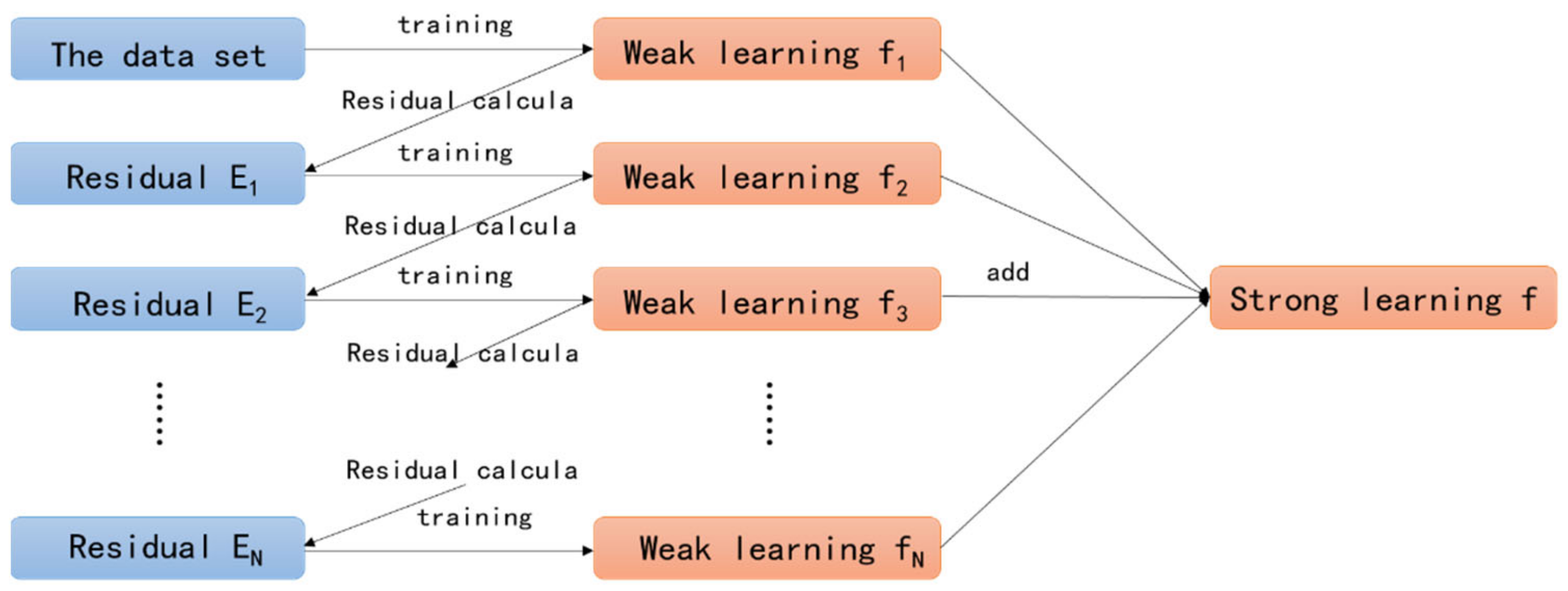
Figure 1. The Structure of the eXterme Gradient Boosting (XGBoost) Algorithm.
Mathematics 09 00476 g001
Figure 2. Numerical Model of the 1.5 Stage Turbocompressor.
Mathematics 09 00476 g002
Figure 3. Distribution of the aerodynamic force on the blade.
Mathematics 09 00476 g003
Figure 4. Procedure of Aerodynamic Modeling.
Mathematics 09 00476 g004
Figure 5. Comparison between XGBoost Model and Computation Fluid Dynamics (CFD).
Mathematics 09 00476 g005
Figure 6. Pressure Contours of the Blade: (a) CFD; (b) XGBoost Model.
Mathematics 09 00476 g006
Figure 7. Error Contour for Pressure.
Mathematics 09 00476 g007
Figure 8. Unsteady aerodynamic value of the blade section.
Mathematics 09 00476 g008
Figure 9. Aerodynamic Force at the Blade Pressure Side: (a) CFD; (b) XGBoost Model.
Mathematics 09 00476 g009
Figure 10. Aerodynamic Force Error on Blade.
Mathematics 09 00476 g010
Figure 11. Aerodynamic Force on the Blade: (a) CFD; (b) XGBoost Model.
Mathematics 09 00476 g011
Figure 12. Error Contour for Aerodynamic Force.
Mathematics 09 00476 g012
Figure 13. Graphs of Error at different testing data: (a) CFD; (b) XGBoost Model.
Mathematics 09 00476 g013
Table 1. Parameters for XGBoost Model Initialization.
Max-DepthLearning-Raten-EstimatorsObjective
400.3560Reg:gamma
Table 2. Parameters in XGBoost Model after Adjustment.
Max-DepthLearning-Raten-EstimatorsObjective
190.1160Reg:gamma
Publisher’s Note: MDPI stays neutral with regard to jurisdictional claims in published maps and institutional affiliations.