Modeling Precious Metal Returns through Fractional Jump-Diffusion Processes Combined with Markov Regime-Switching Stochastic Volatility

Abstract

This paper is aimed at developing a stochastic volatility model that is useful to explain the dynamics of the returns of gold, silver, and platinum during the period 1994–2019. To this end, it is assumed that the precious metal returns are driven by fractional Brownian motions, combined with Poisson processes and modulated by continuous-time homogeneous Markov chains. The calibration is carried out by estimating the Jump Generalized Autoregressive Conditional Heteroscedasticity (Jump-GARCH) and Markov regime-switching models of each precious metal, as well as computing their Hurst exponents. The novelty in this research is the use of non-linear, non-normal, multi-factor, time-varying risk stochastic models, useful for an investors’ decision-making process when they intend to include precious metals in their portfolios as safe-haven assets. The main empirical results are as follows: (1) all metals stay in low volatility most of the time and have long memories, which means that past returns have an effect on current and future returns; (2) silver and platinum have the largest jump sizes; (3) silver’s negative jumps have the highest intensity; and (4) silver reacts more than gold and platinum, and it is also the most volatile, having the highest probability of intensive jumps. Gold is the least volatile, as its percentage of jumps is the lowest and the intensity of its jumps is lower than that of the other two metals. Finally, a set of recommendations is provided for the decision-making process of an average investor looking to buy and sell precious metals.

1. Introduction

It is well known that gold and silver behave as safe-haven investment instruments. Investors usually use gold and silver to hedge economic slowdown or crisis periods since they perform better than stocks and other financial assets in conditions of high volatility [1,2]. However, shocks or extraordinary events can also affect the size and intensity of jumps in the volatility of precious metal returns, which investors should consider in their decision-making process. Investors should also consider that the return on metals may be low compared to those of other financial assets, and their participation in portfolios should be limited.

With regard to the relationship between the price of gold and its production, in Blose and Shieh [3], it is mentioned that Keynes [4] developed and assessed a model that related the mining industry with the contemporary gold prices. As a matter of fact, Keynes cites that “the relation between the price and the mining output of gold is negative in the short term”. However, this relation is not always applicable; for instance, Selvanathan and Selvanathan [5] showed that, in a five-year period, gold production increased 1% alongside its price, which demonstrates, in contrast, a positive relationship in the short term.

Regarding research on the modeling of the behavior of precious metal returns, Arouri et al. [6] investigated the potential of structural changes and long memory properties in returns and the volatility of the four major precious metal commodities traded on the Commodity Exchange (COMEX) markets (gold, silver, platinum, and palladium). Likewise, Tsolas [7] dealt with mutual fund performance evaluation in terms of operational and portfolio management efficiency, implemented with a sample of precious metal mutual funds. Moreover, He et al. [8] proposed a bi-variate copula-based approach to analyze and model the multi-scale dependence structure in the precious metal markets. Moreover, Pierdzioch and Risse [9] used multi-variate random forests to compute out-of-sample forecasts of a vector of the returns of the four precious -metal prices and compare the multi-variate forecasts with uni-variate out-of-sample forecasts implied by the random forests independently fitted to every single return series. On the other hand, Naeem et al. [10] tested the existence of regime changes by using Markov-switching Generalized Autoregressive Conditional Heteroscedasticity (MS-GARCH) models to explain the volatility of the four precious metals and fit several models with different regimes to the log-returns of each precious metal to test the in-sample analysis of volatility. Finally, Morales and Andreosso–O’Callaghan [11] investigated the nature of volatility spillovers between precious metal returns over 15 years (from 1995–2010), with their attention focused on the market behavior during the Asian and global financial crises.

This paper attempts to model the dynamics of gold, silver, and platinum returns from 1994 to 2019 using a stochastic volatility model that combines fractional jump-diffusion processes with continuous-time homogeneous Markov chains. Under this framework, risk variables, such as idiosyncratic volatility and volatility of volatility, are incorporated into a stochastic volatility model. The empirical analysis consists of calibrating a stochastic volatility model for the returns of each metal, in which the Markov regime-switching model treats volatility as the state variable. This will provide information on the probabilities of staying in low or high volatility or going from low to high volatility and vice versa for each metal. Subsequently, the Hurst exponent is estimated to explore the presence of long-memory behavior or the mean reversion of the returns. Finally, a Jump-GARCH model is estimated to find out on the intensity of the jumps of the volatility returns.

The main characteristics that distinguish this work with respect to the current literature on the subject are as follows: (1) it provides an overview of precious metals to learn more about them as assets in order to better understand their market behavior rather than just using a price database of metals to estimate a statistical model; (2) it develops and calibrates a non-linear, non-normal, multi-factor, time-varying risk stochastic volatility model that adequately replicates the dynamics of the daily returns of precious metals during the period 1994–2019; (3) it presents, through empirical comparative analysis, the relevant information regarding the magnitude and intensity of price jumps, as well as the behavior of the volatility through its changes, which is useful for an investor’s decision-making process when they intend to use precious metals as safe haven instruments in their portfolios; and (4) it provides a set of recommendations for investor decision-making.

This paper is organized as follows: the next Section presents a short overview of three precious metals (gold, silver, and platinum); Section 3 states the main assumptions and sets up the model; Section 4 describes the data; Section 5 carries out the calibration of the proposed stochastic volatility model and discusses the empirical results obtained; finally, Section 6 provides the conclusions and acknowledges the limitations of this study.

2. An Overview of Gold, Silver, and Platinum Prices

A brief overview of the precious metals examined in this study is provided below to learn more about them as assets in order to better understand their behavior in the market through their production and demand.

Gold is a malleable, conductive, ductile, non-destructive, brilliant, and beautiful metal. These characteristics have made it a coveted item in almost every civilization. As a precious metal, it has been a symbol of power, importance, and beauty. Its history as an item of trade started 6000 years ago, and it has since been a consistent source of wealth and medium of exchange.

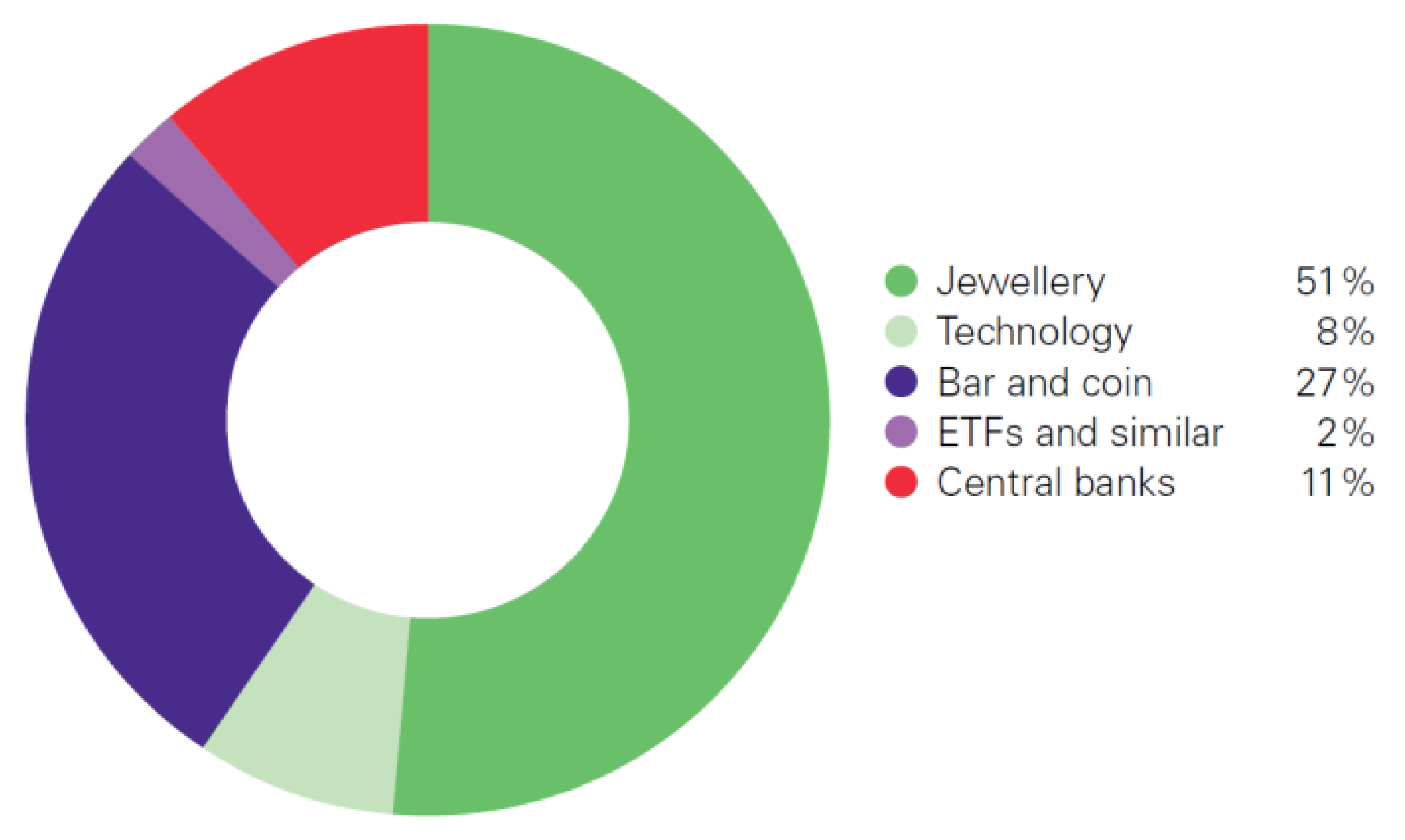
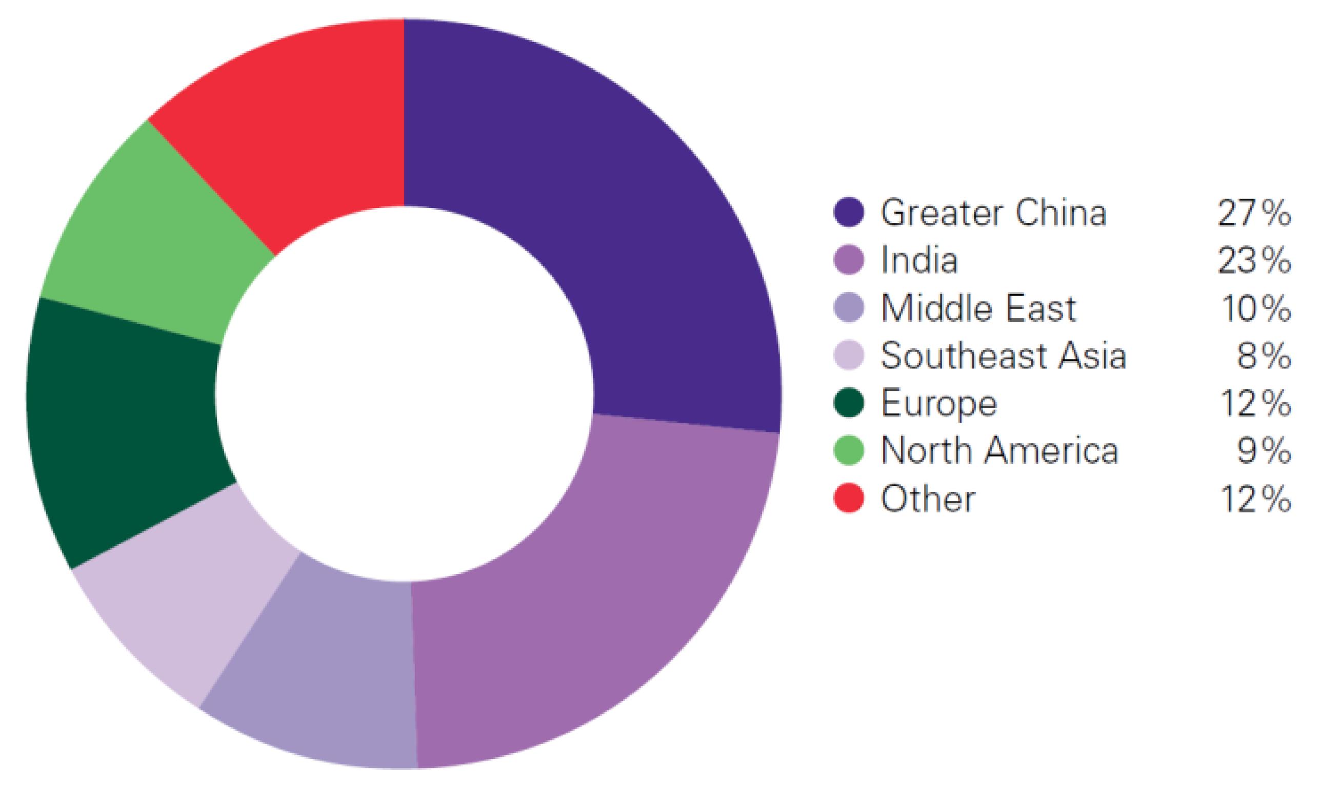
Figure 1 shows the average percentages of the various uses of gold in terms of central bank assets, bars, coins, jewelry, and technology, as well as its function as an underlying asset in financial instruments and contracts, over the last 10 years. Observe in Figure 1 that gold is supplied from mining and scrap, which comes from recycling old jewelry and some electronics goods. Moreover, Figure 2 shows the average demand for gold by region in the same period.

When investors seek higher returns, they routinely expose themselves to higher risks. In times of crisis, gold allows investors to manage risk and preserve their capital efficiently [13]. Gold gives stability to portfolios, and it is a hedge against the volatility of the US Dollar [14]. Adding gold to an investment portfolio reduces risk and increases the average return. Precious metals have the capability to hedge adverse market conditions, since they perform better during high volatility periods [15].

On the other hand, the sentiments of traders are a component of intra-day volatility, suggesting that extreme excitement or fear causes volatility jumps in gold returns, bearing implications for asset management [16]. The Financial and Economic Attitudes Revealed by Search (FEARS) index can predict short-term stock market reversals and increments in volatility [17], and when considering these conditions, having gold in an investment portfolio helps reduce market risk.

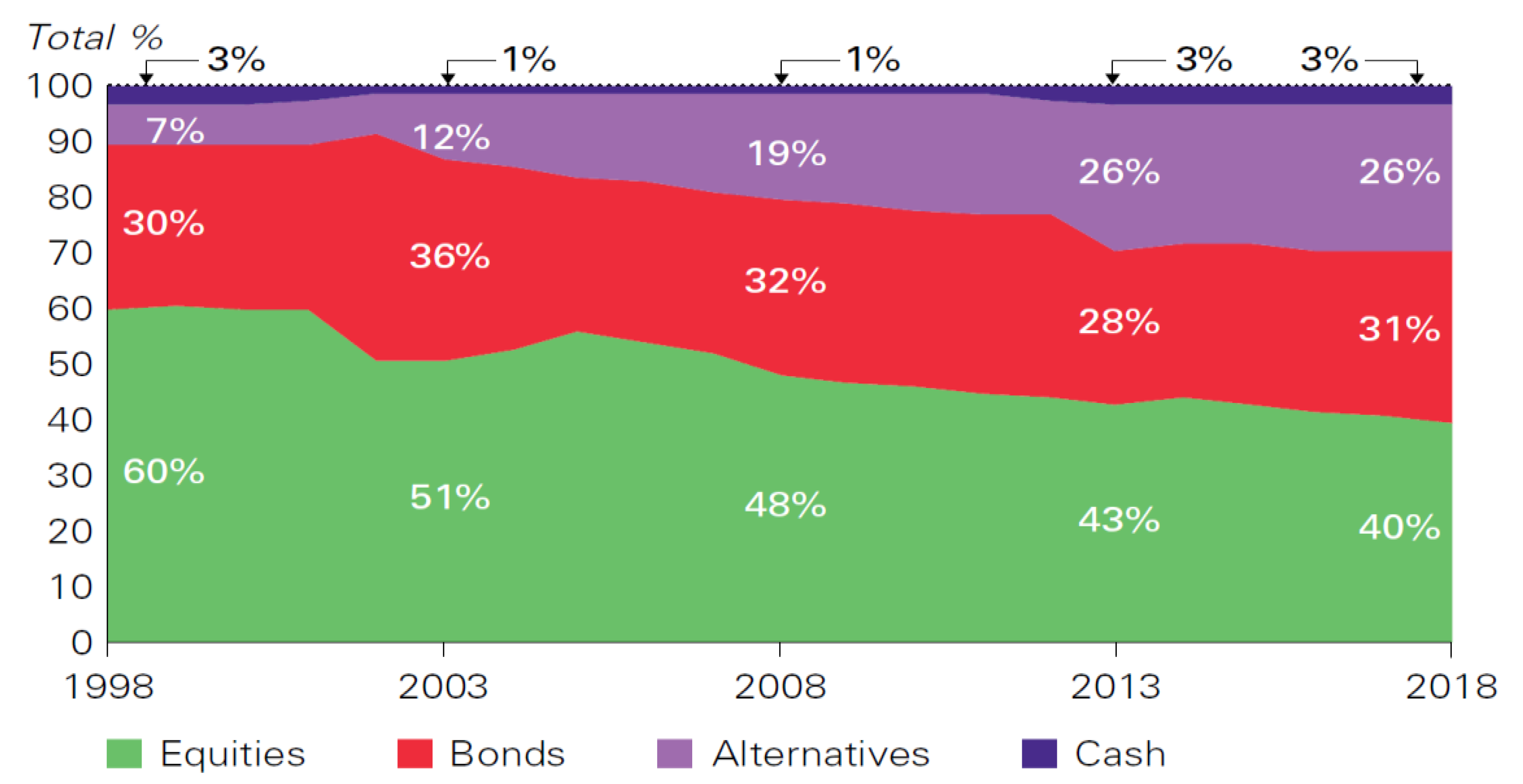
Investment assets, such as equities, bonds, and derivatives in financial markets, have increased steadily in the last few years, causing an increment in the market risk of the financial system (see Figure 3). This increasing exposure to risk creates the need for safe haven investment instruments, such as gold, which is used most of the time to hedge against stock markets in crisis periods [18,19].

On the other hand, several studies have shown that the Volatility Index (VIX) often hedges the volatility of stock markets better than gold [20]. There is evidence that volatility is asymmetric to the stock markets, implying that returns and volatility are negatively correlated. A fall in the price of a stock causes an augment of its financial leverage and volatility [21]. If the correlation between volatility and equity prices is negative, then investors can make the decision to buy or sell equity according to VIX. Investing for a long period with diversification diminishes the effects of volatility, especially during equity market downturns.

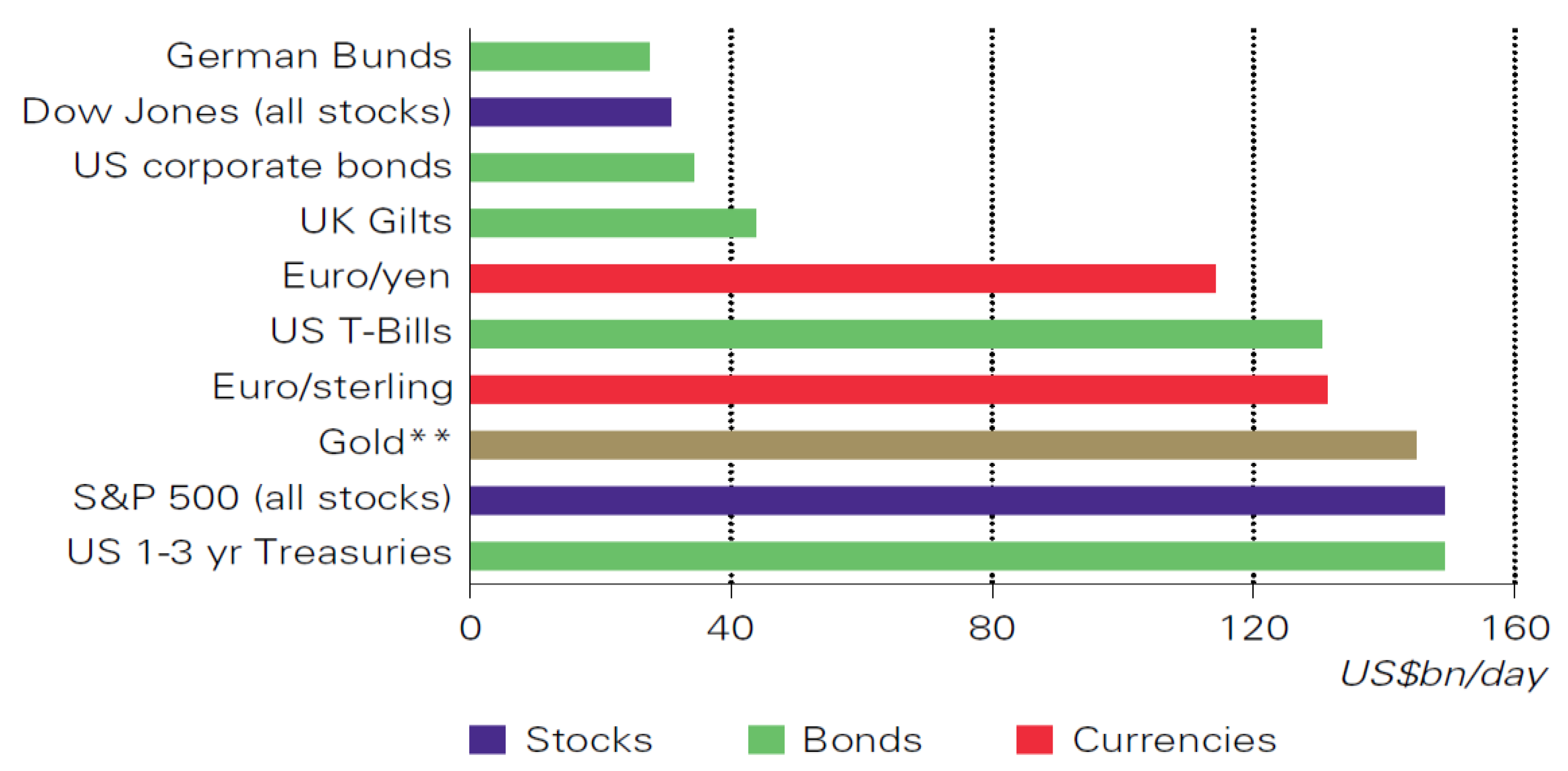
Gold is mainly traded on the following markets: the London Over the Counter (OTC) market, the Commodity Exchange (COMEX) New York Market, the Tokyo Commodity Exchange (TOCOM), the three Shanghai Exchanges, the Multi Commodity Exchange (MCX) at India, the Dubai market, and the Istanbul market. The biggest market is COMEX, with 34.5 billion USD in gold traded per day. Figure 4 compares the average daily trading of several assets with gold in US dollars [22].

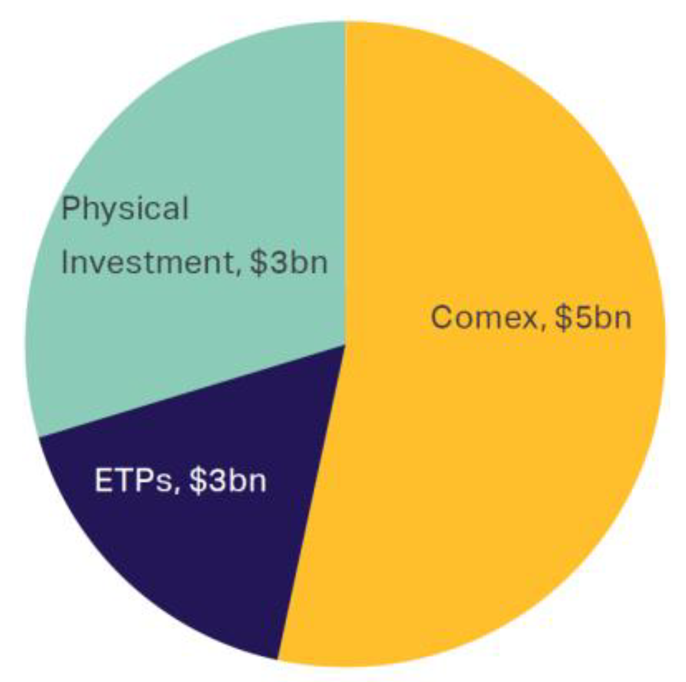
The trading of silver is mainly carried out in the USA and India. Silver investment can be carried out in the Commodity Exchange (COMEX) in the USA (COMEX is the primary futures and options market for trading metals) in physical investment (mostly related to bars and coins), and in exchange traded products (ETPs). The relative proportions of the trading markets of silver are shown in Figure 5.

In 2019, the net long position on the commodity exchanges (COMEX) of the silver future market reached their maximum point and the exchange trade product (ETP) had a new record. The Focus Bullion Coin Survey shows that silver physical investment increased by one-third year after year [23].

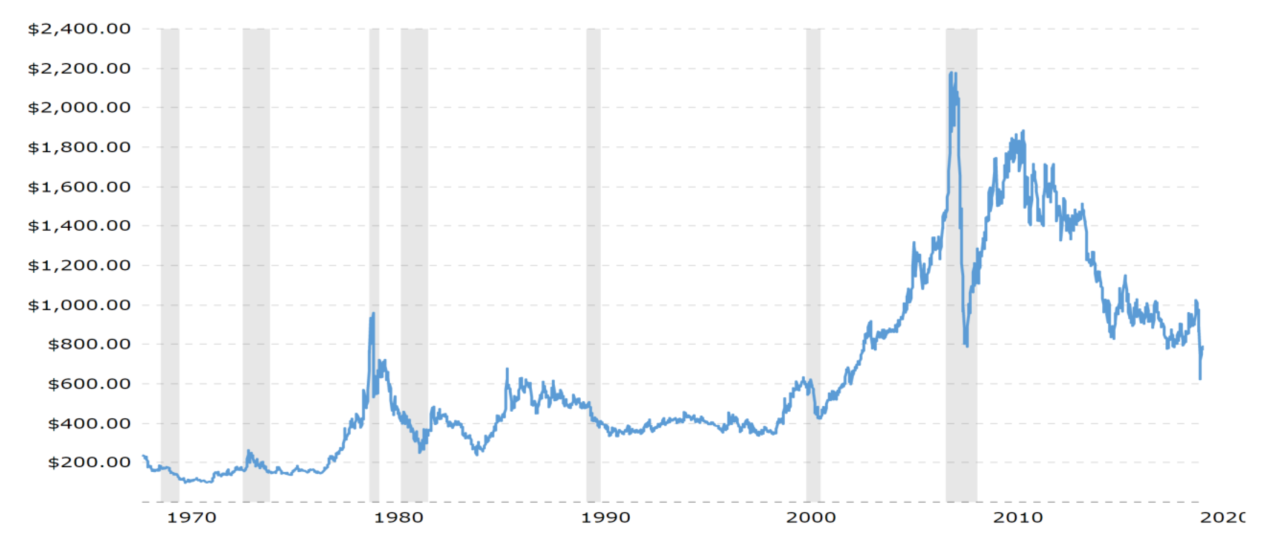
In the 1820s, Colombia was the major producer of platinum in the world. In the 1880s, platinum was discovered in Ontario, Canada, and Canada became the world’s major platinum supplier after World War I. In the 1920s, a South African farmer discovered the metal in a riverbed, and nowadays, South Africa is a world leader in platinum production. Finally, in 1973, the price of platinum began to increase due to the Arab oil embargo.

Figure 6 shows that the platinum price increased from 106 USD in 1973 to 801 USD in 1978 (up 655%), due to the OPEC embargo. In the 1980s, volatility was high and the price of the metal oscillated between 801 USD and 265 USD; after that, in the 1990s, the price was stable at around 400 USD. From October 2001 to March 2008, the price increased considerably from 435 USD to 2041 USD (up 369%); however, due to the mortgage crisis that began in the US in October 2008, the price dropped to 802 USD (down 60%). At the beginning of 2009, the price recovered and manifested a positive trend until August 2011, reaching a value of 1884 USD (up 134%); after this, the price started to fall until the present time, and it has not yet recovered its high level.

Platinum is a dense, malleable, ductile, corrosion-resistant, and highly unreactive metal, with a high melting point. Platinum is used for jewelry and catalytic converters in vehicle engines. In the oil industry it is used to extract gasoline from crude oil, in the technology sector it is used to create hard disks for computer storage, and in the medical industry it is used for dental fillings, pacemakers, and chemotherapy treatments for various cancers.

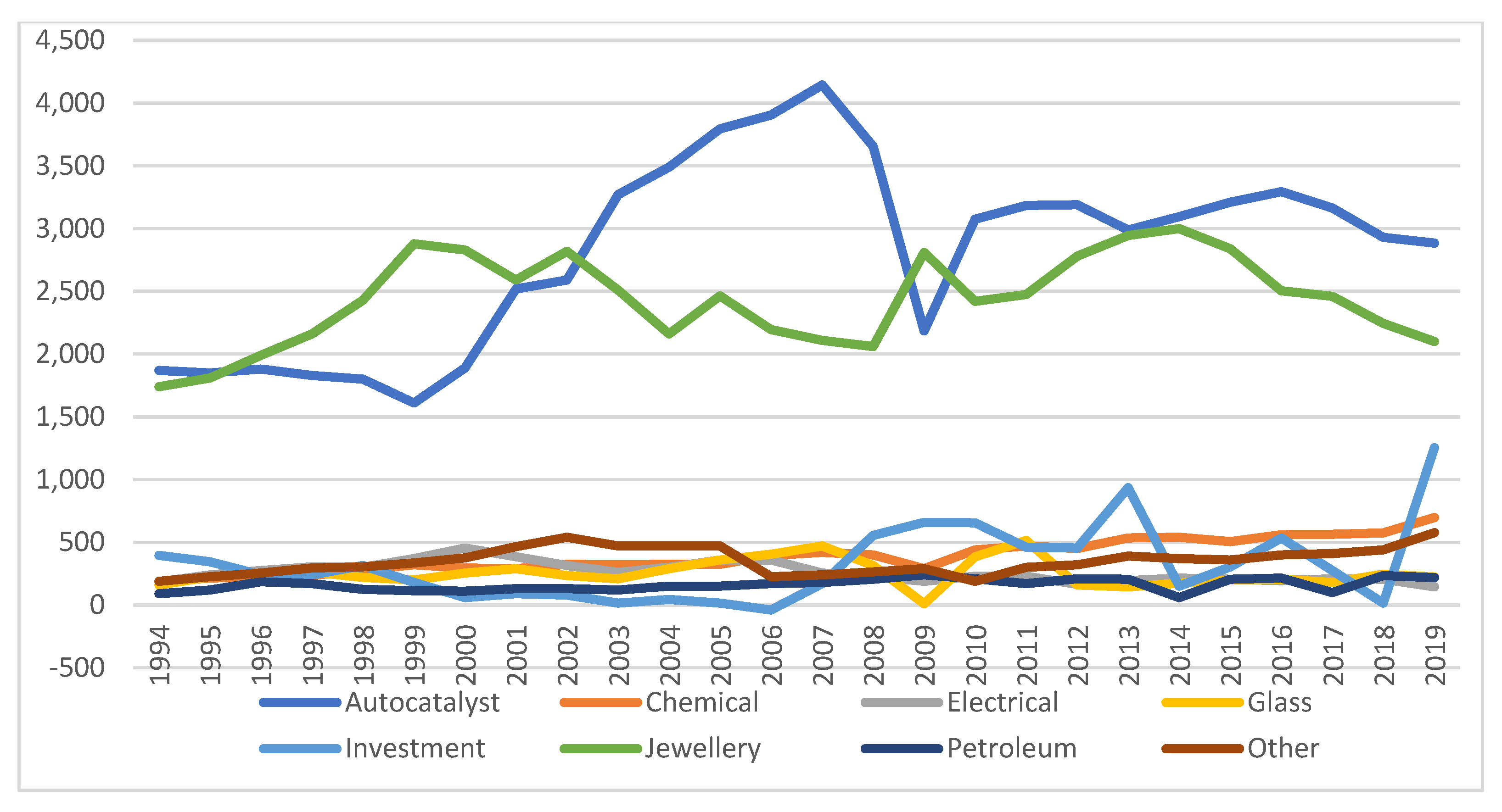
The platinum industries that have exhibited a higher demand for platinum from 1994 to 2019 are the auto-catalyst and jewelry industries. The platinum demand from the auto-catalyst industry doubled from 2000 to 4000 thousand ounces (koz) from 2000 to 2007, when the mortgage crisis started. After that, the demand decreased to almost 2000 koz, and it has recovered slowly to 2800 koz without reaching its maximum level since. The investment industry has increased investment from 500 to 1250 koz from 1994 to 2019; it has been the only industry to exhibit such a raise (see Figure 7).

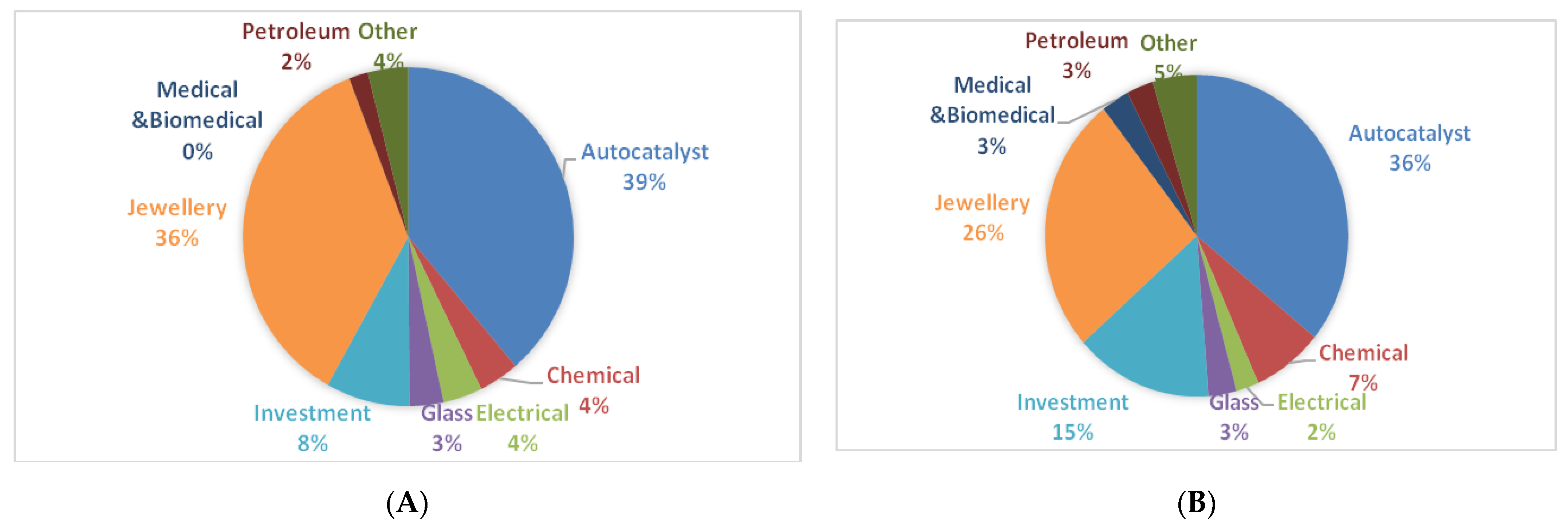
From 1994 to 2019, the participation of the auto-catalyst industry in terms of total platinum demand has decreased by 3%, the participation of the jewelry industry has diminished by 10%, and the participation of the electrical industry has been cut in half. On the other hand, the chemical and investment industries have doubled their investments. Finally, the medical and biomedical industries have shown new participation since 2005 with 3% of the market, respectively. Figure 8 shows the demand of platinum in 1994 and 2019, respectively; the demand changes between the beginning and the end of the study period are shown.

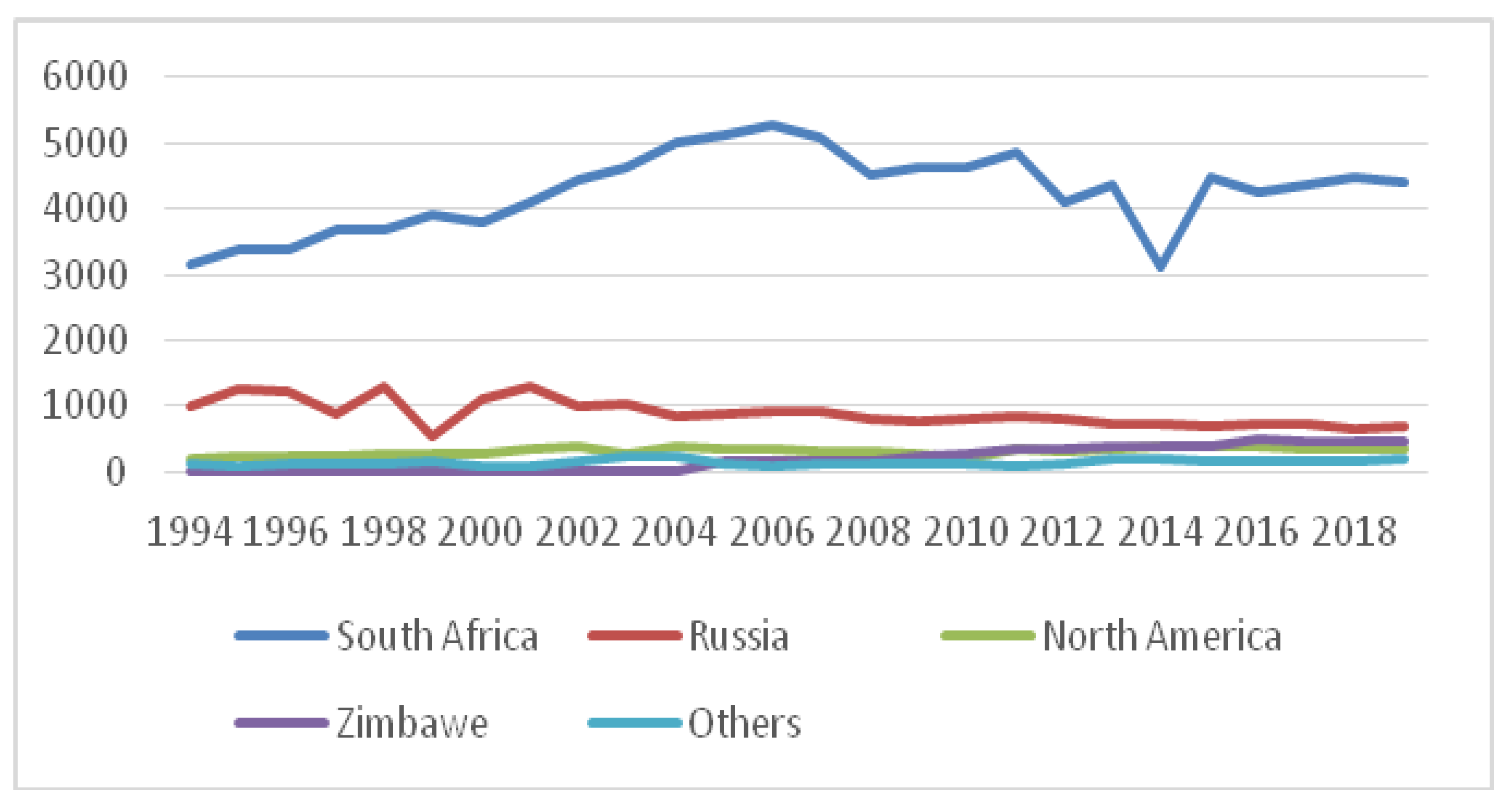
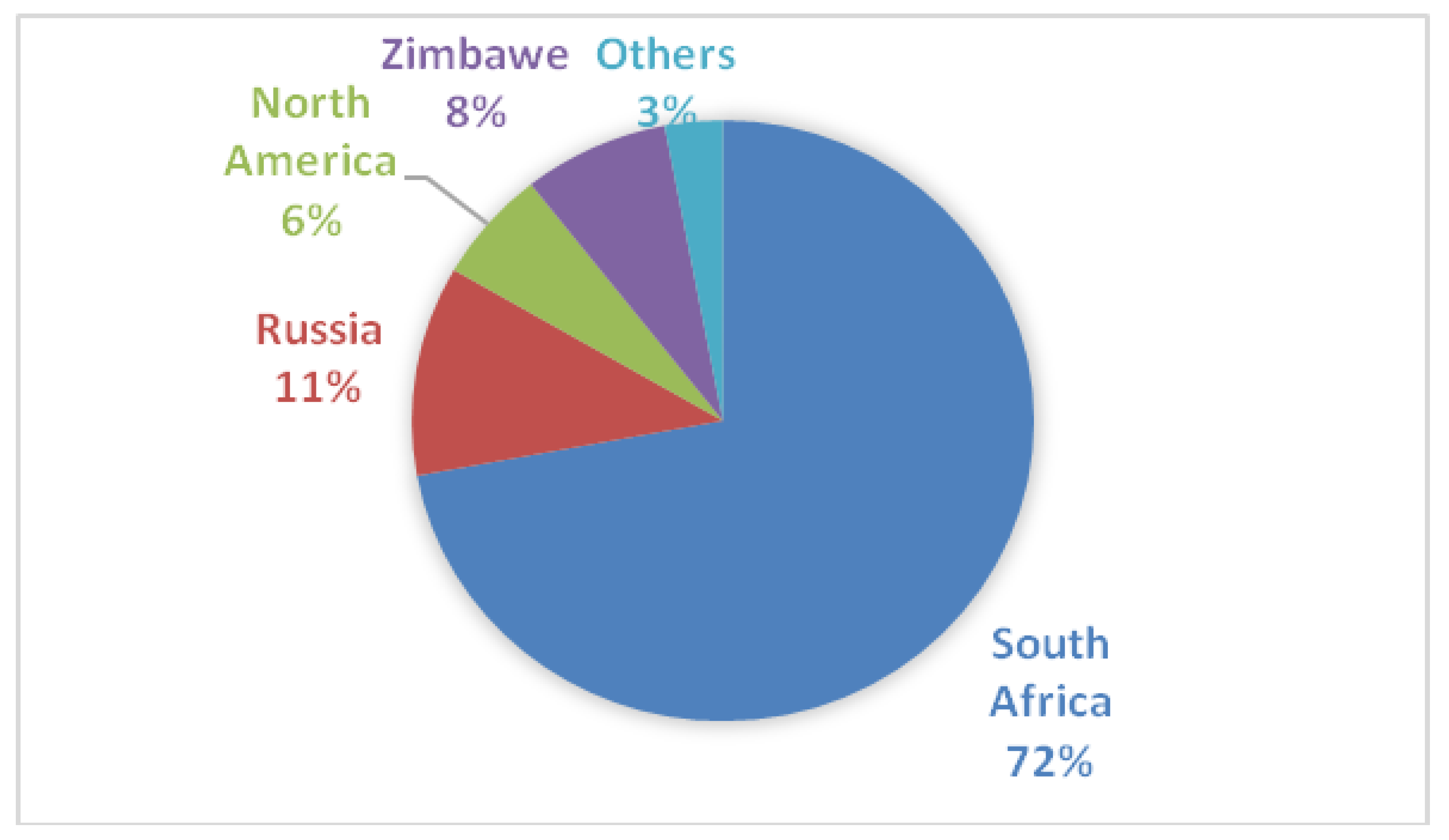
The largest supply of platinum is in South Africa; South Africa’s supply has gone from 3160 to 4415 koz from 1994 to 2019, and it currently represents 72% of the world supply. The second largest supplier is Russia, with 11% of the world supply, and the third largest supplier is Zimbabwe, with 8% of the world supply. The supply of Russia has decreased from 1010 to 690 koz, and, contrarily, Zimbabwe’s supply has increased from 0 koz in 2004 to 465 koz in 2019. See Figure 9 and Figure 10 for the dynamics of the supply between 1994 and 2019 and the producers’ participation, respectively.

3. Setting of the Model

Durham and Park [25] proposed a Markov regime-switching model of both the volatility of the volatility and the intensity of the jump to determine the skew and kurtosis of the derivatives (options). Moreover, Vallejo–Jiménez and Venegas–Martínez [26] developed a model that explains the dynamics of an individual asset that is driven by multiple jumps, fractional Brownian motion, and regime-switching stochastic volatility; see also [27,28,29]. In our proposal of a multifactor risk model that is aligned with these past studies, the returns of the metals are driven by fractional Brownian motion ($\mathrm{d}{B}_{1t}^H$ and $\mathrm{d}{B}_{1t}^H$), combined with Poisson jumps ($\mathrm{d}{N}_t$) and modulated by a Markov chain, with the volatility states listed as follows:

$$\mathrm{d}{y}_t=\left(\mu -\frac{1}{2}{v}_t^2\right)\mathrm{dt}+v_t\mathrm{d}{B}_{1t}^H$$

(1)

$$\mathrm{d}{v}_t=a\left(b-v_t\right)\mathrm{d}t+{\sigma }_i\mathrm{d}{B}_{2t}^H+\gamma \mathrm{d}{N}_t$$

(2)

$$E=\left\{{\sigma }_1,{\sigma }_2\right\}$$

(3)

$$\mathrm{Cov}\left(\mathrm{d}{B}_{1t}^H,\mathrm{d}{B}_{2t}^H\right)=0$$

(4)

$$\mathrm{Cov}\left(\mathrm{d}{N}_t,\mathrm{d}{B}_{it}^H\right)=0,i=1,2$$

(5)

where $\mathrm{d}{y}_t$ is the dependent variable determined by the metal returns, $\mathrm{d}{B}_{1t}^H$ and $\mathrm{d}{B}_{2t}^H$ are independent fractional Brownian motions, $H$ is the Hurst exponent, $\mu$ is the mean (trend parameter) of the returns, $\mathrm{d}{N}_t$ is a Poisson process, $v_t$ is the volatility of the metal returns (idiosyncratic volatility), ${\lambda }_t$ is the intensity parameter associated with the jump process that describes the number of jumps per unit of time, ${\sigma }_i$ is the volatility of volatility of the metal returns, $\mathrm{d}{v}_t$ is the change in volatility of the returns, a is the speed adjustment parameter of volatility, b is the long-run mean (mean reverting),$\gamma$ is the mean jump size, and E is the set of states (low volatility (${\sigma }_1$) and high volatility (${\sigma }_2$)); other works dealing with jump-diffusion processes can be found in [30,31,32]. The first equation explains the dynamic of the metal returns in terms of a trend plus idiosyncratic volatility, which is associated with fractional Brownian motion. The second equation states that volatility is stochastic and is explained through a mean reverting process, plus the volatility of volatility associated with fractional Brownian motion, plus a term of Poisson jumps with expected jump size $\gamma$. Finally, it is worthwhile to point out that the covariance of $B_t^H$ is non-stationary, since

$$\mathrm{E}[B_t^H{B}_s^H]=\frac{1}{2}\left(|t{|}^{2H}+|s{|}^{2H}-|t-s{|}^{2H}\right)$$

which, clearly, leads to Var[$B_t^H]=t^{2H}.$

3.1. Fractional Brownian Motion and Hurst Exponent

Fractional Brownian motion $B_t^H$ is defined on a fixed probability space with its augmented filtration ($\mathsf{\Omega },F,{\left(F_t\right)}_{t\in \left[0,T\right]},\mathrm{and}P),\mathrm{and}Hϵ\left(0,1\right)$ is the Hurst coefficient [33]. If the Hurst coefficient ($H$) is bigger than $½$, it determines the long-term memory of a time series. In this case, it describes the irregularity of the motion, predicts asset return, and reflects the auto-correlation on returns. It is worth mentioning that if $H\ne ½,\mathrm{then}{B}_t^H$ is not a semi-martingale [34], and when H is smaller than $½$, it reflects a mean reverting effect. In summary: If H = $½$, the process is a Brownian motion or a Wiener process; if H > $½$, the increments are positively correlated (indicating a long memory); finally, if H < ½, the increments are negatively correlated (indicating a mean reverting effect); see also [35].

In this sense, Hurst’s (1951) parameter, or Hurst’s exponent, was proposed to study the behavior of the Nile River over a long period of time in order to determine the water level and the optimum dam sizing. The exponent H has been used to solve problems related to fractals, chaos theory, spectral analysis, long memory process, and mean reverting processes. It is related to fractal dimension, where a basic pattern is repeated at multiple scales, and it is defined in terms of the rescaled range. Let N be the full length of a time series and define $n$ = N, N/2, N/4, … Then, the Hurst exponent is defined through

$$\mathrm{E}\left[{\left(R/S\right)}_n\right]=A{n}^H$$

(6)

$\mathrm{as}n\to \infty$, or

$$\ln \mathrm{E}\left[{\left(R/S\right)}_n\right]=\ln \left(A\right)+H\ln \left(n\right)$$

where ${\left(R/S\right)}_n$ is the rescaled range, $\mathrm{E}[·]$ is the expected value, $A$ the constant of proportionality, and $H$ is the Hurst exponent. In order to estimate H, the mean of each n-th partial time series $x_i,\mathrm{i}=1,2,\dots ,n$, is first calculated:

$$M_n=\frac{1}{n}{\displaystyle \sum }_{i=1}^n{x}_i$$

(7)

Then, a mean adjusted series is defined:

$$w_t=x_t-M_n,t=1,2,\dots ,n$$

(8)

Next, the cumulative deviation is computed:

$$U_t={\displaystyle \sum }_{i=1}^t{w}_i,t=1,2,\dots ,n$$

(9)

Subsequently, the range is calculated through:

$$R_n=\max \left(U_1,U_2,\dots ,U_n\right)-\min \left(U_1,U_2,\dots ,U_n\right)$$

(10)

The standard deviation is also computed:

$$S_n=\sqrt{\frac{1}{n}{\displaystyle \sum }_{i=1}^n{\left(x_i-M_n\right)}^2}$$

(11)

Finally, the rescaled range is defined by:

$${\left(\frac{R}{S}\right)}_n=\frac{R_n}{S_n}$$

(12)

3.2. Fractional Brownian Motion Modulated by a Markov Chain

The fractional Brownian motion ($B_t^H$) can be modulated by a Markov regime-switching process, as seen in [36], which is a non-linear time series model that integrates multiple structures to confirm the behavior of a state variable in different regimes. The change of regime or state is called a transition, and the probabilities of change are called transition probabilities. The process is defined through a transition probability matrix (P) of changing from state ${\sigma }_i$ to state ${\sigma }_j$:

$$P=\left(\begin{array}{cc}{p}_{11}& p_{12}\\ p_{21}& p_{22}\end{array}\right)$$

A Markov process has the property that the present state only depends on the immediate past state. A Markov chain could be in discrete or continuous time; in our case, it is continuous and time homogeneous.

3.3. The Proposal and Its Relationship with Autoregressive Conditional Heteroscedasticity ARCH and Jump-GARCH Models

This part briefly reviews the ARCH and GARCH models. The ARCH(q) model is useful to explain the trend of large residuals to cluster together, as in [37], and is given by:

$$v_t^2=\omega +{{\displaystyle \sum }}_{i=1}^q{\alpha }_i{\epsilon }_{t-i}^2,\omega , {\alpha }_i>0,$$

(13)

where $v_t^2$ is the conditional variance, $\omega$ and ${\alpha }_i$ are unknown parameters, and ${\epsilon }_{t-i}^2$ is the lag of the random error term.

In the GARCH model, the variance term depends on the lagged variance as well as the lagged square residuals. It allows for the estimation of different types of persistence in volatility [38]. The GARCH(p,q) model is represented by:

$$v_t^2=\omega +{{\displaystyle \sum }}_{i=1}^q{\alpha }_i{\epsilon }_{t-i}^2+{{\displaystyle \sum }}_{i=1}^p{\beta }_i{v}_{t-j}^2,\omega , {\alpha }_i, {\beta }_i>0,$$

(14)

where $v_t^2$ is the conditional variance, $\omega$, ${\alpha }_i$, and ${\beta }_i$ are unknown parameters, ${\epsilon }_{t-i}^2$ is the square of lag of the random error term, $v_{t-j}^2$ is the j-lag of the variance, ${\alpha }_i$ is the component of the influence of random error in previous periods, and ${\beta }_i$ is the component of the variance in the previous period.

In order to extend the above approach, the Jump-GARCH is an alternative for modeling the dynamics of metal returns when sudden and unexpected jumps occur [39]. In this case, two stochastic innovations ($I_{t,1}$ and $I_{t,2}$) capture the dynamic of the returns with no jump and with jump, respectively. The innovations $I_{t,1}$ and $I_{t,2}$ are independent and satisfy:

$$I_t= I_{t,1}+ I_{t,2}.$$

(15)

The first innovation means that the market stays normal (no jump); thus:

$$I_{t,1}=v_t{u}_t, u_t~N\left(0,1\right)$$

(16)

and

$$\mathrm{E}\left(I_{t,1}| y_{t-1}\right)=0.$$

(17)

The second innovation describes an unexpected jump when an unusual event occurs. That is to say, the metal return is affected by an unexpected event. The distribution of jumps follows a Poisson process with the intensity parameter ${\lambda }_t$; hence:

$$I_{t,2}=N_t-\mathrm{E}\left(N_t|y_{t-1}\right)=\gamma -\theta {\lambda }_t,N_t|y_{t-1}~P\left({\lambda }_t\right)$$

(18)

and

$$\mathrm{E}\left(I_{t,2}| y_{t-1}\right)=0$$

(19)

where $y_t$ stands for the metal return, $N_t$ is the jump component, $\gamma$ is the jump size, ${\lambda }_t$ is the jump intensity, and $\theta$ is the component associated with jump intensity. The Poisson process $N_t$ with the intensity parameter ${\lambda }_t$ satisfies:

$$\mathrm{P}\left\{\mathrm{one}\mathrm{jump}\mathrm{during}\mathrm{d}t\right\}=\mathrm{P}\left\{\mathrm{d}{N}_t=1\right\}={\lambda }_t\mathrm{d}t+\mathrm{o}\left(\mathrm{d}t\right)$$

(20)

$$\mathrm{P}\left\{\mathrm{none}\mathrm{jump}\mathrm{during}\mathrm{d}t\right\}=\mathrm{P}\left\{{\mathrm{dN}}_{\mathrm{t}}=0\right\}=1-{\lambda }_t\mathrm{d}t+\mathrm{o}\left(\mathrm{d}t\right)$$

(21)

Hence,

$$\mathrm{P}\left\{\mathrm{more}\mathrm{that}\mathrm{one}\mathrm{jump}\mathrm{during}\mathrm{d}t\right\}=\mathrm{P}\left\{\mathrm{d}{N}_t\ge 1\right\}=\mathrm{o}\left(\mathrm{d}t\right)$$

(22)

where $\mathrm{o}\left(\mathrm{d}t\right)/\mathrm{d}t\to 0$ as $\mathrm{d}t\to 0\mathrm{and}{\left(\mathrm{d}t\right)}^2.$ Then,

$$\mathrm{E}\left[\mathrm{d}{N}_t\right]=\mathrm{Var}\left[\mathrm{d}{N}_t\right]= {\lambda }_t\mathrm{d}t$$

(23)

$$\mathrm{Cov}\left({\sigma }_t{u}_t, N_t\right)=0$$

(24)

It is important to point out that Equation (2) in our proposal is related to a Jump-GARCH in terms of mean (1,1) and $\alpha + \beta$ is the level of persistence; see also [40].

4. Data Description

The most traded metals are gold, silver, and platinum. The data was taken from Bloomberg on a daily basis. The sample period of analysis is from January 1994 to October 2019, or 6542 days. The purpose of this research, as mentioned before, is to calibrate a stochastic model that captures the dynamics of the returns and the volatility of these main metals over economic crises and world-relevant events.

The idiosyncratic volatility and one-day lagged returns are used to describe the dynamics of volatility for each metal. By applying the Eviews software, the Markov regime switching is estimated. The RATS software is also used to estimate the Jump-GARCH parameters. Finally, R platform statistical analysis is used to estimate the Hurst exponent.

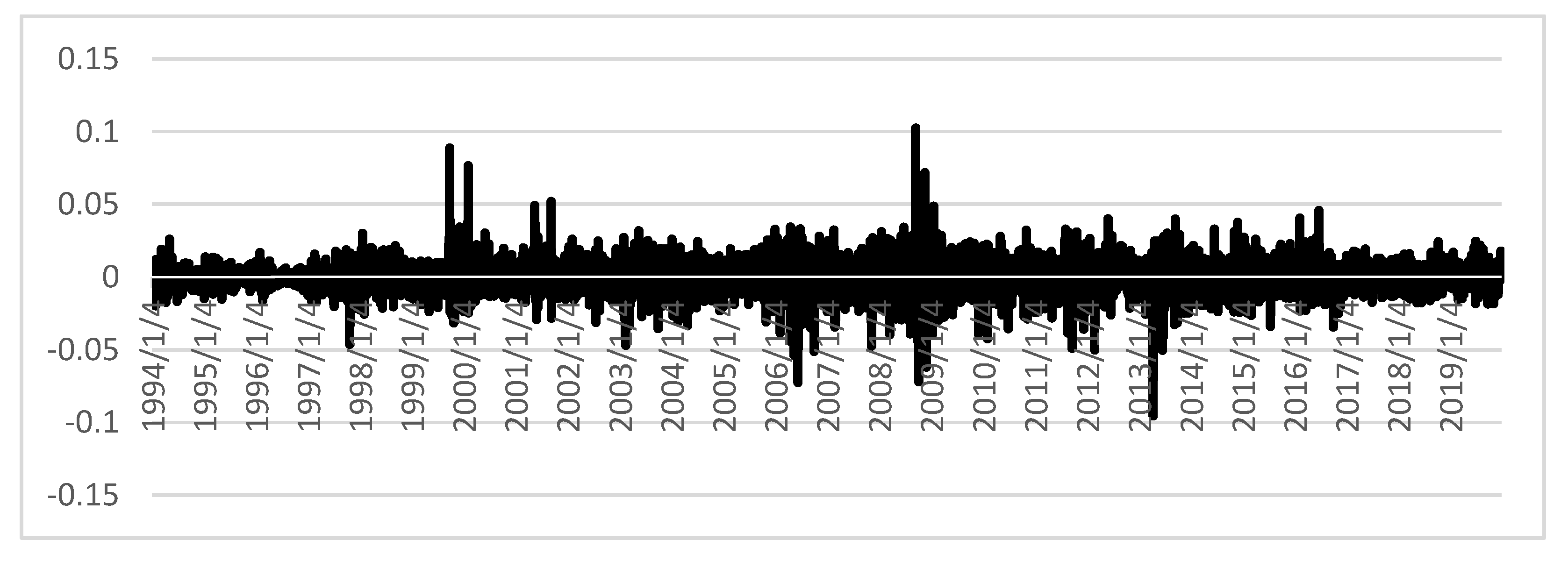
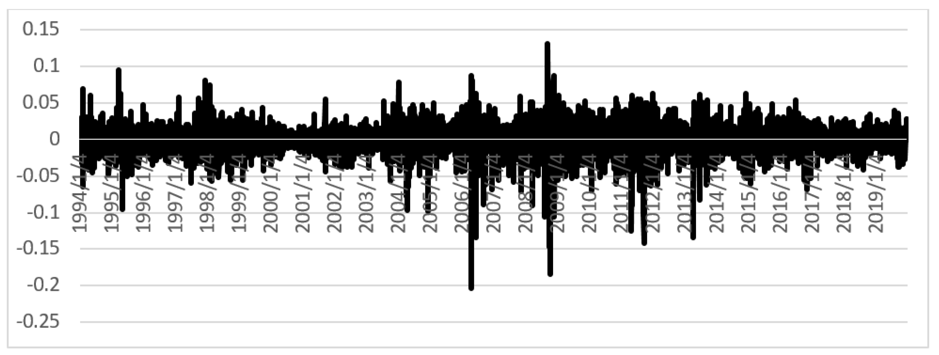
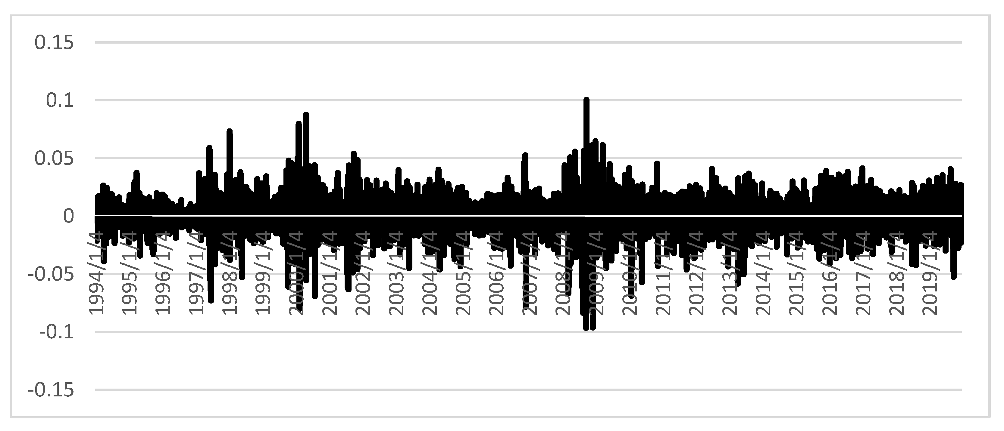
Figure 11, Figure 12 and Figure 13 show the gold, silver, and platinum returns between 1994 and 2019. The y-axis stands for the returns and the x-axis stands for the dates. These charts show the volatility and the unexpected jumps.

Figure 11 shows the daily returns of gold from 1994–2019. The higher jumps are those in September 2008, when the stock market collapsed (resulting in a positive jump), and in April 2013, close to the end of the quantitative easing (QS) programs in the US (resulting in a negative jump).

Figure 12 presents the returns of the silver price and shows huge jumps in September and October 2008 due to the effect of the mortgage sub-prime recession, followed by jumps in March and September 2011 due to the Eurozone debt crisis. The end of the quantitative easing (QE) of US programs caused a jump in April 2013.

Finally, Figure 13 shows that the higher jumps in platinum price occur during the sub-prime mortgage recession in September and December 2008. In February and May 2002, smaller jumps appeared because of the dotcom bubble, and in June 1997 and January 1998 the jumps are due to the Asian financial crisis.

Previous graphs show that silver presents the highest intensity of jumps on a scale from 0.14 to −0.20; therefore, this metal presents a higher volatility that the other two. Gold shows the lowest volatility on a range from 0.10 to −0.07, which indicates a high intensity of jumps. That is to say, the number of jumps per unit of time is high. Finally, notice that platinum maintains its jump intensity within a scale of 0.10 and −0.10.

5. Model Calibration

In this section, the models for the dynamics of the metals’ returns will be calibrated by estimating Markov regime-switching models, calculating the Hurst coefficients, and estimating Jump-GARCH models.

5.1. Markov Regime-Switching Empirical Analysis

Markov processes are defined by the probability of a future state judging by the present information; the immediate past state determines the probability of the present state. In our study, the estimation of the Markov regime-switching model describes the probability of changing from low to high volatility and vice versa. The estimations of the transition probabilities for gold, silver, and platinum are shown in

Table 1. Transition probabilities of the Markov regime-switching model of metals.

Parameters	Gold	Silver	Platinum
p11	0.868538	0.879089	0.880861
p12	0.131462	0.120911	0.119139
p21	0.784871	0.757485	0.738367
p22	0.215129	0.242515	0.261633

Source: Authors’ own elaboration, with Bloomberg data [22] and Eviews software.

. The results from the Markov regime-switching statistical test are shown in

Table 2. Statistical test of Markov Regime-Switching.

Dependent Variable	Independent Variables	z-Statistic Prob.
Gold Return	Gold Return (−1) ***	(0.0001)
	Volatility Idiosyncratic ***	(0.0001)
Silver Return	Silver Return ***	(0.0001)
	Volatility Idiosyncratic ***	(0.0001)
Platinum Return	Platinum Return (−1) ***	(0.0041)
	Volatility Idiosyncratic ***	(0.0001)

Source: Authors’ own elaboration, with Bloomberg data [22] and Eviews software. *** indicates statistical significance at the 1% level, ** indicates statistical significance at the 5% level, and * indicates statistical significance at the 10% level.

.

Table 1 shows that gold, silver, and platinum have a higher probability to stay in low volatility than in high volatility, directly opposite the tendency of stock indexes. The probability of changing from low to high volatility and vice versa is similar for the three metals. They have a larger probability of changing from high to low volatility, (around 75%) than from low to high volatility (with an average of 12%); gold reacts more than silver and platinum. Table 2 shows the significance of whether our hypothesis is not rejected according to the confidence levels of 99%, 95% or 90%. The z-statistic is used to quantify the statistical significance. Due to the fact that probability is low, the null hypothesis is accepted.

5.2. Empirical Analysis Jump-Diffusion Process and Fractional Brownian Motion

The estimations of the Jump-GARCH models are shown in

Table 3. Estimation of fractional Brownian motion combined with Jump-GARCH.

Parameters.	Gold	Silver	Platinum
$\mu$	0.0002059	0.0001879	0.0001339
$v^2$	0.0100878	0.0178290	0.0134778
$v$	0.0001018	0.0003179	0.0001817
%J	50.05000	51.42260	51.16808
$\lambda$	0.000015	−0.000123	0.000066
$\theta$	−0.012899	−0.020930	−0.034856
$\gamma$	0.0000004	0.000001	0.000001
$\alpha$	0.044488	0.041714	0.062117
$\beta$	0.956454	0.955138	0.931742

Source: Authors’ own elaboration, with Bloomberg data [22] and RATS software.

. As can be seen, the jump percentages (%J) are similar for the three metals, though silver has the highest percentage with a little difference. Silver and platinum have the highest jump sizes, and only silver shows an negative jump intensity with $\mathsf{\lambda }$ −0.000123. Gold has the highest mean return ($\mathsf{\mu })$, while platinum has the lowest. The standard deviation ($\nu$) is the highest for silver and the lowest for gold. For all metals, α + β is very close to 1, which indicates a high level of persistency. Finally the component $\mathsf{\theta }$ (associated with jump intensity) is negative for all metals, which means that most of the jumps are negative.

According to Table 3, an important result is that silver reacts more than the other two metals and is the most volatile with the highest standard deviation, the highest probability of jumps, and the most intense jumps. In contrast, gold is the least volatile metal, its percentage of jumps is the lowest, and the intensity of its jumps is lower than that of the other metals.

On the other hand, the results on Hurst’s exponent show that H is higher than 0.5 for the three metals, as can be seen in

Table 4. Summary statistics of fractional Brownian motion (Hurst exponent).

Hurst Coefficient	Gold	Silver	Platinum
$H$	0.567016	0.539623	0.544126

Source: Authors’ own elaboration, with Bloomberg data [22] and R programming.

. This means that metals’ returns have correlation and trend. That is to say, they follow a pattern over a period of time and their returns have long-memory behavior.

The Hurst exponent can be considered as a measure of persistence when its value is greater than 0.5, reflecting auto-correlation on returns. In this case, the Hurst exponent can be viewed as an indicator of the predictability of the “likeness” aspect associated with returns, rather than as a direct prediction of returns. The highest value of $H$ was observed for gold (0.567016) and the lowest was observed for silver (0.539623). This can be useful information for an investor’s decision-making process when they are looking to incorporate precious metals into their portfolios. Of course, there is a possibility that the Hurst exponent is being misinterpreted as evidence for long-term memory, since these values are close to 0.5, and the Brownian motion should be used instead as a model for the dynamics of returns. However, the Jarque–Bera test strongly rejects normality for the returns of all precious metals, as shown in

Table 5. The Jarque–Bera test on returns.

	Gold Returns	Silver Returns	Platinum Returns
Skewness	−0.086530	−0.323918	−1.004701
Kurtosis	11.04598	8.125494	13.31026
Jarque-Bera Statistics	17651.92	7274.239	30072.03
Probability	0.000000	0.000000	0.000000

Source: Authors’ own elaboration, with Bloomberg data [22] and Eviews software.

.

6. Conclusions

The novel value of this research has been the use of a non-linear, non-normal, multi-factor time-varying risk stochastic volatility model to adequately describe and explain the returns of various precious metals. The empirical results showed that all metals maintain low volatility and have long memory most of the time, which means that past returns have an effect on current and future returns. Along with this, all metal returns (gold, silver, and platinum returns), have a higher probability to maintain low volatility than exhibit high volatility. All of them have a higher probability to change from high to low volatility than from low to high volatility, as shown in the Markov regime-switching models.

Regarding the Jump-GARCH model, the percentage of jumps (%J) is similar for all three metals. Silver and platinum have the largest jump sizes, silver has the highest intensity of its negative jumps, and the standard deviation is highest for silver and lowest for gold. In summary, silver reacts more than the two other metals and is the most volatile, with the highest standard deviation, the highest probability of jumps, and the most intense jumps. In contrast, gold has the lowest volatility, a lower jump percentage, and its jump intensity is lower than that of the other metals. The Jump-GARCH model provides signals to investors and traders for the buying and selling of metals in the markets; it shows the level of market reaction and the intensity of jumps, which allows them to know the degree of the effect of news on the studied metals.

The outcome of the Hurst coefficient $H$ for the fractional Brownian motion $B_t^H$ is H > ½ for all metals, meaning that the increments are positively correlated and have long memory. Thus, data have correlation and the market has a trend, which reflects auto-correlation on returns. A shock on the returns of metals is long-lived; thus, past events have an effect on the present and future returns. Because of the long memory of gold, silver, and platinum returns, future returns can be predicted using the past returns; thus, portfolio managers may include metals in their stock markets portfolios to develop futures strategies according to past returns.

All three metals are predictable in terms of the “likeness” aspect associated with performance. In this regard, it is important to note that gold has attractive investment characteristics for the average investor. Gold has a much larger liquid market driven primarily by investment and the demand for jewelry. The price of gold is less volatile than that of silver and platinum, and the intensity of its jumps is lower than that of the other metals. However, investors should be aware that the returns on metals can be low compared to other financial assets and their holding in portfolios should be limited, particularly in the case of silver, as it has the highest intensity of negative jumps and reacts much more than the other two metals. In short, gold behaves more like a safe haven asset in crises and extraordinary events.

In summary, it can be said that our proposal of modeling precious metal returns through fractional jump-diffusion processes combined with Markov regime-switching stochastic volatility was capable to describe the dynamics and explain the behavior of metals’ returns, and foresee important implications to investors.

It is important to mention some limitations of this research. For example, the trend parameter is constant over time. One possible solution to this is to incorporate another stochastic differential equation into the model for its dynamics. Another solution to correct this problem would be to modulate the trend with an in-homogeneous Markov chain. A second limitation is that it does not incorporate sector volatility.

Finally, our future research agenda is to extend the proposed model to incorporate jumps not only in idiosyncratic volatility, but also in sector volatility and the volatility associated with systemic risk.