Abstract
The global exploring feature of the surrogate model makes it a useful intermedia for design optimization. The accuracy of the surrogate model is closely related with the efficiency of optima-search. The cokriging approach described in present studies can significantly improve the surrogate model accuracy and cut down the turnaround time spent on the modeling process. Compared to the universal Kriging method, the cokriging method interpolates not only the sampling data, but also on their associated derivatives. However, the derivatives, especially high order ones, are too computationally costly to be easily affordable, forming a bottleneck for the application of derivative enhanced methods. Based on the sensitivity analysis of Navier–Stokes equations, current study introduces a low-cost method to compute the high-order derivatives, making high order derivatives enhanced cokriging modeling practically achievable. For a methodological illustration, second-order derivatives of regression model and correlation models are proposed. A second-order derivative enhanced cokriging model-based optimization tool was developed and tested on the optimal design of an automotive engine cooling fan. This approach improves the modern optimal design efficiency and proposes a novel direction for the large scale optimization problems.
1. Introduction
With its inherent benefit of uncertainty prediction, Kriging and cokriging methods have drawn much attention in recent decades. An overwhelming number of approaches emerge posteriori to the design and analysis of computer experiments (DACE) approach [1,2], including surrogate-based optimization (SBO), surrogate-assisted evolutionary algorithms [3]. Some recent approaches show impressive performance for high dimensional problems with 30–200 design variables [4,5]. However, the improvement on model accuracy remains to be further studied. Studies on model reliability, either from local or global points of view [6,7], follows two main paths. First, by applying different training strategies [8], one tries to improve the local precision of the surrogate model, especially that of the optima neighborhoods, so-called “design space exploitation”. This is particularly useful, and at times indispensable for large-scale optimization. Recent studies also deal with different strategies to find the balance between exploration and exploitation by using multi-fidelity [9] and an ensemble of different surrogate methods [10]. Second, by introducing assistant information such as derivatives to the original dataset, the surrogate model can be improved. The most typical development concerns the integration of the adjoint method and the gradient-enhanced cokriging model in the aerodynamic shape optimization [11]. What is worth noticing here, the co-Kriging method [9], which uses the correlations between several models of various fidelities, is not the same with the cokriging method in this study which interpolates the samples and the associated derivatives at the same time, generating one-single surrogate model. One remarkable advantage of adjoint method lies in the independence of the number of design variables, making this approach an appropriate choice for high-dimensional problems. However, the gradients obtained from this method depend on some given objective functions because the reversal mode differentiation is used, consequently, adding new objectives requires a new adjoint-state evaluation. Furthermore, for the modeling of multimodal functions, the higher is the order of derivatives used, the better is the model accuracy [12,13].
Yet the computational cost, being the main obstacle, limits the application of the high-order approach. With a classical differentiation method such as finite differences, depending on the discretization scheme, the number of evaluations required multiply by a factor of n (the number of parameters) for the differentiation of every higher degree of order. Although the higher accuracy brought by the derivatives, the total computational effort remains quasi-identical with a classical derivative-free method. The integration of derivatives in a surrogate-modeling process is not efficient unless the derivatives can be obtained in a cheap way.
This paper introduces the integration of the sensitivity analysis method and the derivative enhanced cokriging surrogate model. The former allows us to pursue the high-order derivatives in a cost effective way. The latter can make the best of the auxiliary information and generate a far-more accurate surrogate model.
The sensitivity analysis is to obtain the sensitivity of the output to the input by using their differential relations [14]. In the optimal design, the sensitivity analysis is often used for the quantitative study of the variation of the objective functions in response to some perturbations of the parameters. It can also be used to evaluate the robustness of the optimal design, performed at the post-processing phase. However, the implementation of sensitivity associated methods to the modeling phase is also feasible. The sensitivity information at the design site can be used to build the surrogate model. This is particularly useful for the problems featuring important nonlinear characteristics.
For the aerodynamic shape optimization, there are several ways to compute the sensitivities of design variables: finite difference method, complex step method [15,16], automatic differentiation and sensitivity equation method. E.Colin, Etienne, Pelletier and Borggaard brought forth the idea of continuous sensitivity equation method, illustrating how to obtain a fast solution of a flow field and its sensitivities with the finite element method [17]. The sensitivity equations are formed by implicitly differentiating the Navier–Stokes equations. Mahieu et al. proposed the generalized formulation of this approach which allows computing the first and second order derivatives of any parameters [18]. Please note that some key problems remain unsolved due to the high nonlinearity of Navier–Stokes equations and the derivability difficulty of turbulence model used in Reynolds-averaged Navier–Stokes equations.
A high-order extension of sensitivity equation method has been studied by Aubert, Ferrand et al. [19,20]. Instead of differentiating the governing equations directly, derivatives are computed a direct mode automatic differentiation [21] applied to the discretized reference solutions [22,23]. As with the adjoint-state method, this approach applies its reverse mode to get high-order derivatives. Some non-commercialized tools have been developed, namely Turb’Flow, Turb’opty and Turb’post, which are flow solver, sensitivity solver and flow extrapolation tool respectively. Based on these tools, Soulat has accomplished an aerodynamic shape optimization for a fan system used in the automotive engine cooling module [24]. High order derivatives were used to build a polynomial surrogate model, which can be viewed as an aerodynamic database extrapolated from one single reference design. Taylor expansion was employed for the extrapolation. Optimization based on this model brought a significant reduction of aerodynamic tip loss due to secondary flow. However, only one single reference design has been considered in his study, so the truncation error presented by nature, and the effective region covered by the model is limited to a certain radius. By introducing derivative-assisted cokriging method, it is possible to enlarge the covered region.
In summary, to make the best of their respective advantages, the high order sensitivity method and cokriging surrogate model are integrated in current studies. The high-order sensitivity approach is firstly introduced, then its integration with Hessian-enhanced cokriging model is presented. This methodology is employed for the aerodynamic shape optimization of an automotive engine cooling fan.
2. Sensitivity Approach in CFD Simulation Based Aerodynamic Shape Design
At stationary equilibrium state, the Navier–Stokes equations can be expressed in the following form:
With F the flux vectors: the mass, the momentum and the energy in terms of conservative variables , and the transport of turbulent variables such as k and used in Reynolds-Averaged Navier–Stokes equations (RANS) [20]. P stands for the design parameter, which can be either geometric or physic parameter. Differentiation of this equation with respect to P yields:
It can also be written:
in which is the first order variation of q by varying P by .
The Jacobian matrix allows writing the order differentiation as . The right part is the flux vector variation in function of . Hence the equation can be represented in this form:
The order differentiation can be constructed by recursively differentiating Equation (4).
Please note that the linear system is based on the Jacobian matrix G, which is usually available in a classical implicit Computational Fluid Dynamics (CFD) solver. The high-order derivatives can then be used to reconstruct the flow fields corresponding to parameter variations , as shown in Figure 1.
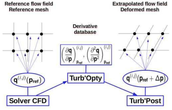
Figure 1.
Diagram of parametrization process (Ref: [19]).
The implementation of this methodology requires a coherence between the algorithm used for the discretization of the Navier–Stokes equations and that of the resolution of sensitivity equations. However, the derivability difficulty presented in the discrete RANS equations when using SST-K- turbulence model with Roe discretization scheme. Negative dissipation term has been found during the resolution of sensitivity equations, leading to a negative turbulent viscosity, which caused the crash of the solver. Positivity preservation study has been carried out but there is not yet any constructive conclusion.
For a methodological illustration, this study adopts an alternative approach for the derivative computation by using the finite difference method. This does not deprive the originality of the methodology. To respect the original idea of the sensitivity method, a mesh deformation method is applied [25]. The latter relies on a morphing technique which calculates the mesh(nodes) displacements with a Radial Basis Function (RBF) approach [26,27]. The mesh deformation is a RBF type propagation out of the displacements of some user-defined control points which are usually positioned on the boundaries of computational domain. A such type deformation is illustrated on a 2-D surface mesh in Figure 2, where the dots refer to the control points. Displacements are attributed to the inner control points, the outer ones are fixed deliberately. The displacements of mesh nodes are calculated following a radial basis function defined a priori. This technique is employed to obtain deformed mesh of an automotive engine cooling fan blade (Figure 3).
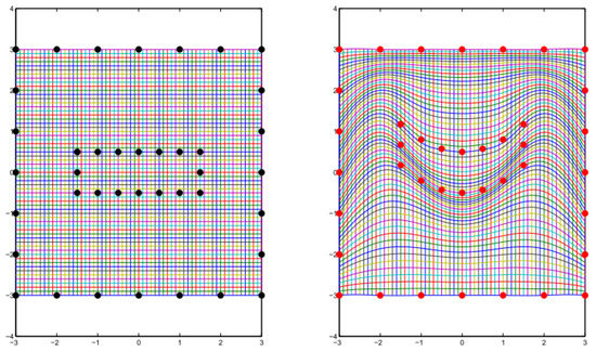
Figure 2.
Mesh deformation driven by control points (Ref: [26]).
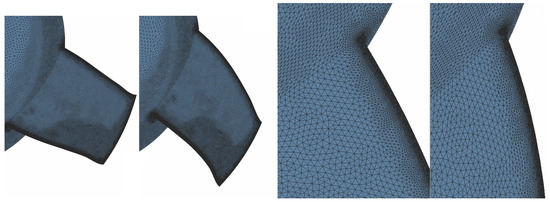
Figure 3.
Deformation example: sweep angle variation and the zoomed view to the trailing edge.
One single reference mesh is used for one geometrical configuration. Derivatives can be deduced from the results of some new CFD simulations based on deformed meshes. Compared with the finite difference discretization scheme which parametrizes the geometrical configuration directly, followed by a re-meshing process for each new configuration, the mesh deformation approach deals with one single reference mesh, which conserves the total mesh element number and assures the similar discretization of the computational domains.
Figure 3 compares the original surface mesh (on the left) with a deformed mesh (on the right) following a variation of sweep angle. As it is shown from the global view of the blade and local zoomed view to the trailing edge, the refinement levels are preserved, the total mesh element number remains unchanged after the deformation. The deformation of the blade surface mesh is propagated into the computational domain in a RBF pattern as presented before. The derivative calculation takes the same method presented in the reference [28].
3. Derivative-Enhanced Cokriging Method
Surrogate models of three objectives in function of three parameters (see for details in section of “Case study”), can be built out of the database constituted of the CFD and sensitivity analysis results. Different approaches are available, being either parametric or non-parametric [29]. A polynomial model, based on one single reference design, is taken in a previous study [28]. The cokriging method which interpolates several reference designs and their derivatives, can effectively reduce the truncation error and enlarge the covered region.
By assuming a stochastic process of all the interpolations upon the given sample points, the Kriging method models an unknown function through a mean function and a covariance function. It is often the best linear unbiased prediction from some given evaluations, i.e., the prediction error is minimized. The regression model can be considered to be the mean function of all the possible interpolation functions subject to the existing evaluations. Constant average functions are frequently used as the regression model [30,31]. However, once differentiated, high-order derivative-enhancing effect will be erased. On the contrary, a too high order regression model may provoke some unrealistic local oscillation similar to that of Runge phenomenon while equidistant samples are used for the interpolation [32,33]. Experience shows the second order polynomial function is good compromise and it is, thereforem chosen for current study which uses databases up to second order. The regression matrix for a cokriging model consists of a regression part and a differentiated part which takes the following form:
where and are respectively the first order and second order derivatives of the regression matrix .
Correlation Model
The correlation model reflects the spatial correlations between the points of the design site. The prediction error of a Kriging model is assumed to follow a random process, a careful choice of law of probability for this process is essential. Generally, the law of probability is unknown. Assumption has to be made in order to characterize the covariogram in the random field. The Gaussian model is the most-frequently used, which assumes a the second-order stationary conditions of the design site, making Kriging modeling a Gaussian process. The interpolation properties primarily depend on the local behavior of the random field. Near to the origin, the Gaussian model shows a quadratic behavior. For the sake of derivability, it is chosen for current study, the correlation between two samples can be expressed as:
where is the Euclidean distance between two samples and at dimension. Where denotes the dimension index, are the index of the sample point.
The correlation model can be established by evaluating a hyper-parameter namely , which can be obtained by the minimizing of the following function:
where m is the number of sample points, is the standard deviation of the stochastic process of the samples, R is the correlation matrix.
The correlation matrix can be written:
where stands for the covariance, S represents the normalized design site, interpreted by the position of sampling points in a unit hyper-cube, and are the differentiated forms of S.
The covariance between any reference point and all the rest reference points is given by:
where denote the dimension indices, denote the sample indices, is the variance of the sample.
An example of the correlation between the first order derivative of dimension for point and the first order derivative of dimension for point is given:
Once the regression matrix and the covariance matrix R are calculated, the cokriging model can be deduced:
where is the correlation vector between any design to be predicted and existing reference points, Y is the response matrix, regression coefficient vector can be calculated by a least square estimation which gives:
Variance is given by:
The derivatives calculated by the sensitivity approach is integrated with the above described derivative-assisted cokriging method. Models can be built for all the objective functions. Optimization can be performed based on these models. This methodology is applied to the optimal design of an automotive engine cooling fan.
4. Case Study
An automotive engine cooling fan, as shown in Figure 4, has been optimized based on the presented methodology. A reference fan design has been adapted for the particular surrounding of the vehicle underhood, where the downstream flow is radially deviated from its axis by the engine.
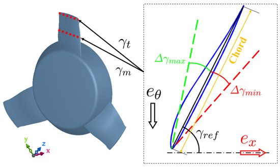
Figure 4.
Geometrical parameter definition.
The pressure rise from upstream to downstream of the fan wheel, the torque T acting on the fan and the aerodynamic efficiency are considered to be objectives to be optimized. The first study has been performed with only one database, details can be found in the work of Zhang et al. [28] and references therein.The three parameters considered are: variations of stagger angles at mid-span and tip as shown in Figure 4, flow rate Q. For simplicity, the variations are illustrated with and for mid-span stagger angle variation and tip stagger angle variation respectively. Derivatives of the three objectives with respect to three parameters are computed based on CFD simulations performed on the deformed mesh.
Two geometrical configurations, functioning at two operating points, generates four reference designs. Based on the derivative-assisted reference data, surrogated models are built and are used for optimizations.
For one single operating point with first and second order derivatives, at most it describes an evolution of order 2. Yet, the characteristic curve in Figure 5, which describe two objectives: and efficiency at different flow rates, shows an inflection at the operating point (flow rate 2500 m/h) and a linear evolution at the flow rates higher than 2500 m/h, a behavior which can only be approximated by a curve of order 3 or higher. With one single flow rate, one cannot reproduce this characteristic for such an extended range. By associating two points, however, it is possible to depict a characteristic of order 5, hence enlarge the range of extrapolation.
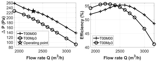
Figure 5.
Reference fan characteristic curves: -Q and -Q. T00M00 and T00Mp3 represent two different geometric configurations. The stagger angle at mid-span of T00Mp3 is more than that of T00M00 (Reference configuration).
Figure 6 illustrates the schema of coupling of different databases. The reference values are 2300 m/h and 2600 m/h for the flow rate, and for the stagger angle at mid-span, the stagger angle at the tip takes its reference relative value . The circles represent the extrapolation from one single reference point, i.e., they are polynomial models. The rectangulars show the coupling of two or four databases. The characteristic curves of the two fans are shown in Figure 5.
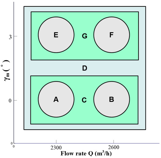
Figure 6.
Metamodeling schema.
With a processor of type Inter(R) Core(TM) i7-2640M, 8G physical RAM, the building of models C and G have consumed about 6 minutes of CPU time, the construction of model D takes about 23 minutes because of the inverse operation of a larger size of covariance matrix R. Time is considerably short comparing with a CFD run, which typically takes more than 1000 CPU hours.
Figure 7 (left) shows the prediction on by the model C, where the stagger angle is fixed at its reference value. The two stars shows the of two reference points. The error bar (red) is given by the surrogate model. CFD evaluations are illustrated with crosses. Notice that the blue line in the model does not pass by all the evaluated points because of all the CFD results, except for the reference ones, are used to calculate the derivatives but not to build the model directly. The error bar shows clearly the error is minimized as approaching the reference points.
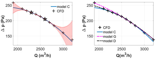
Figure 7.
Comparisons among models C, G and D: -Q. .
Figure 7 (right) shows the comparison of three surrogate models: C, G and D. For the flow rate, the curve of model C and D passes by two reference points m/h and m/h. The curve of model G does not pass by those points, which is originally from the error of second order cross derivative . At high flow rate, model D is closer to model G, but not model C, this fact shows the influence from the dimension of . In fact, has a similar effect with the flow rate. By increasing the , the air incidence is reduced, the blade is discharged, a phenomenon that can also be observed by increasing the flow rate. Model D, which couples four different databases, allows us to obtain more reliable results on a larger range of parameter variation. Hence this model is used to exploit the optima according to different criteria.
4.1. Mono-Objective Optimization Based on Model D
Several optimizations have been done, one of them is the maximization of efficiency by varying all the parameters at their full ranges. The goal of this optimization is firstly to have an idea about the maximum efficiency that can be found in the current design space, secondly to testify this approach of uniting the optimization algorithm and the surrogate model.
The genetic algorithm [34] is used with an initial population of 5000, evaluated on 100 generations. Thanks to the surrogate model, 500,000 evaluations have been done within a few hours, a task which is not achievable by CFD means. What is worth mentioning, the time-cost can be further reduced by using the long term memory assistance approach for evolutionary algorithms where the same solutions are not evaluated again [35]. This will be highly recommended when the number of parameters is higher, which should be considered in the future studies.
The result is shown in Table 1.

Table 1.
Comparison between the reference design and the optimum on efficiency.
To assess the validity of the prediction, the results are compared with a CFD run. The differences are no more than 1% for all the three objectives, an error within the numerical uncertainty of the CFD simulation. Hence this approach is validated for the maximum efficiency design.
The optimization proposes a set of parameters which modifies the reference geometry and eventually leads to the required performance. The analysis of physics helps us to understand the local modification on the flow field by the optimizer.
The pressure distributions on six different radii have been drawn to have a global view of the fan blade charges (Figure 8).
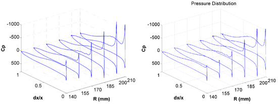
Figure 8.
The pressure distribution at six constant radii.
This graph highlights the strong acceleration at the leading edge of the blade, which gradually amplifies at larger radius. The most important outcome of the optimizer is a discharged blade particularly at the region near the tip.
To better understand the flow structure modification, the radial profile of the axial velocity at about 4 mm downstream of the trailing edge, circumferentially averaged, is mapped out (Figure 9), where the reference fan “Reference” is compared with the efficiency-optimized fan “optimA”.
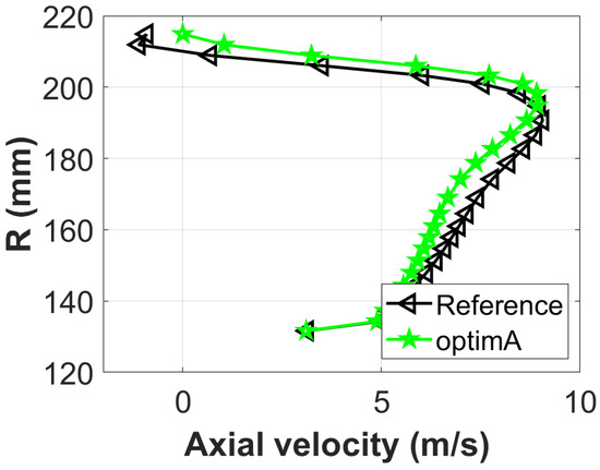
Figure 9.
Axial velocity at the downstream of the fan wheel.
Globally the radial evolution of the axial velocity of the optimum design is similar with that of the reference design. Both of them show a forced vortex characteristic, because only two stagger angles at mid-span and tip are modified. This also explains the similarity between two profiles near the hub. The axial velocity is small near the hub and linearly increases until a radius of 190 mm, beyond which the secondary flow and the wall effect of the shroud predominate. The optimum configuration maintains a null axial velocity at the tip, which allows the blade to work more efficiently at higher radius. This analysis shows the complexity of the flow near the shroud: tip vortex, secondary flow, brutal deviation of inlet velocity from axial to radial, high charges at higher radius. This study is carried out on only two geometrical parameters. According to this analysis, it will be useful to add more parameters such as the stagger angle at the hub section of the blade for the future study.
4.2. Multi-Objective Optimization Based on Model D
Based on model D, a multi-objective optimization has been performed to pursue an optimal design in term of performance at two different operating conditions: m/h and m/h. At nominal operating point 2300 m/h, a higher efficiency is wanted, for 2800 m/h, a higher pressure rise is preferred in order to have an extended range of flow rate. The flow rate corresponding to is called the “transparent” point, beyond which the fan module generates negative pressure rise, bringing extra drag for the vehicle. A transparent point with higher Q value allows vehicle running at higher speed without generating extra drag. According to the fan characteristic curve shown in Figure 5, it is more likely to have a higher flow rate at transparent point if the at 2800 m/h is higher.
Two objectives: efficiency at m/h, namely and pressure rise at m/h, namely , have been considered. The algorithm NSGA-II [36] has been employed with 5000 individuals and 100 generations due to the inexpensive model-based evaluations. For each point, two performance evaluations have been done thanks to the surrogate model, one evaluation at 2300 m/h and the other at 2800 m/h, hence 10,000 evaluations have been done for each generation. The bi-objective Pareto front is illustrated (Figure 10).
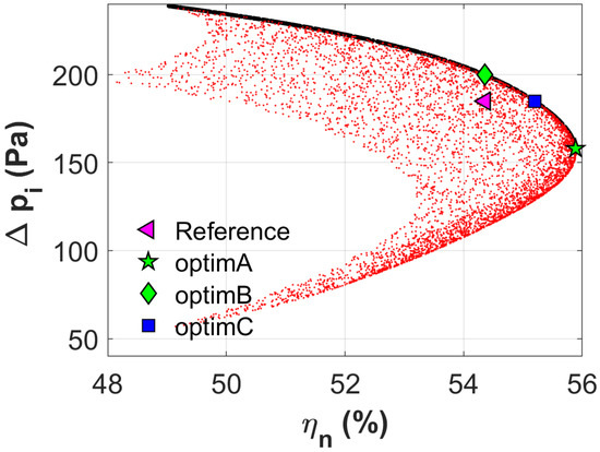
Figure 10.
Pareto front of optimization: maximization of (2300 m/h) and (2800 m/h).
In Figure 10, the initial individuals, marked as red points, form a 2-dimensional projection on the objective surface . The frontiers are clearly depicted, where the Pareto front can be seen on the top-right part, marked with black dots, formed of 502 survived individuals.
In order to illustrate the possible exploitation with the surrogate model, two optima have been adopted on the Pareto front, one favors the transparent point (optimB) and the other valorize the efficiency of nominal condition (optimC). Optimization results are compared with the reference configuration “Ref” in Table 2.
Table 2.
Result of multi-objective optimization at two operating conditions.
The numbers in italics are those values of objectives concerned in this optimization. By keeping the same efficiency with the reference geometry, OptimB manage to raise the pressure rise at 2800 m/h by 15 Pa, or 8.1%. In addition, if the pressure rise at 2800 m/h is kept unchanged, the efficiency at 2300 m/h can be improved by 0.84, or 1.5% higher than the reference configuration. These improvements are analyzed according to the flow structure modifications.
The variation of stagger angles changes the radial distribution of fan load. Comparing to the reference geometry, the optimB shows an important variation of tip stagger angle, which charges the tip with a high incidence, so that a higher flow rate can be accepted. By keeping almost the same stagger angle at the mid-span, the efficiency stays unchanged comparing with the reference geometry. For the optimC, the tip stagger angle has little variation comparing with optimB, but a more important variation at mid-span. This reduces the incidence and eventually augments the (2300 m/h) by keeping the same level of (2800 m/h).
To better understand the optimization result shown on the Pareto front, a Self-Organizing Map (SOM) [37] visualization was created with all the individuals on the Pareto front. SOM can be used to make the connection between design-space and objective-space effectively. It is a type of neural network designed to understand high-dimensional data with help of its low-dimensional representations. Each variable (parameter or objective) is depicted as a two-dimensional map which preserves topological properties of the Pareto optimal solutions. One individual is always found at the same 2-D position from one map to another, distinguished with the other individuals according to their colors, which represent the magnitude of the variable.
In Figure 11, there are four maps which represent the values of two parameters and two objectives on the Pareto fronts. Only negative values are observed on the tip stagger angle plot. All the solutions are kept away from their reference value. By contrast, large variation () is shown for the mid-span stagger angle, the positive values correspond to the individuals which give better efficiency but less pressure rise , the negative values correspond to the individuals which give a less efficiency but a better . A clear correlation can be drawn among three variables: mid-span stagger angle, efficiency and pressure rise . CFD simulations have been performed to validate the optimA and optimC, the maximum relative error is 1.3%, found for the of optimC at 2300 m/h, an error within the numerical uncertainty. The approach is again validated for this multi-objective optimization.
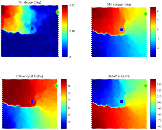
Figure 11.
SOM visualization of Pareto front, optimA (green diamond point) and optimC (blue square point).
5. Conclusions
The integration of the second-order sensitivity method and the cokriging surrogate model was studied in this paper. The derivative-assisted information significantly improve the model accuracy. Optimizations are performed based on established surrogate model. One of the optimization results shows obvious improvements on both the aerodynamic efficiency and the torque for an engine cooling fan. One multi-objective optimum succeeds in enlarging the operating range of the fan, the other manages to keep the same range and improve the efficiency at nominal condition.
The contributions of this paper are twofold:
- The cokriging method can make the best use of the derivatives and significantly improves the surrogate model accuracy;
- The implementation of parameterization tool (Turb’Opty) has been pre-illustrated. The cycle of optimal design can be effectively shortened through low-cost derivatives. This study proves the validity and efficiency of this methodology.
Author Contributions
Conceptualization, Z.Z.; methodology, Z.Z.; software, Z.Z. and M.B.; validation, P.F. and M.H.; writing—original draft preparation, Z.Z.; writing—review and editing, M.B. and P.F.; visualization, Z.Z.; supervision, P.F. and M.H.; project administration, P.F.; funding acquisition, M.H. All authors have read and agreed to the published version of the manuscript.
Funding
This research was funded by “Association Nationale de la Recherche et de la Technologie” (ANRT) in France.
Acknowledgments
The authors acknowledge the supports from CIRT and Fluorem S.A.S.
Conflicts of Interest
The authors declare no conflict of interest.
Abbreviations
The following abbreviations and symbols are used in this manuscript:
| CFD | = | Computational Fluid Dynamics |
| RANS | = | Reynolds-Averaged Navier–Stokes equations |
| RBF | = | Radial Basis Function |
| F | = | Flux over any arbitrary grid cell |
| q | = | Flow variables |
| P | = | Design parameter |
| G | = | Jacobian matrix |
| m | = | Number of sample points |
| n | = | Number of dimensions |
| R | = | Kriging correlation matrix |
| = | Kriging regression matrix | |
| = | Kriging correlation parameter | |
| = | Distance between two samples | |
| S | = | Set of a sampling |
| = | dimension of sample | |
| = | cokriging predictor | |
| = | Regression function for prediction | |
| = | Coefficient vector of regression function | |
| = | Generalized least squares solution of regression problem | |
| r | = | Correlation vector of a design to be predicted |
| Y | = | Kriging objective matrix |
| = | Standard deviation | |
| Q | = | Volumic flow rate |
| = | Pressure variation through fan system | |
| = | Static efficiency | |
| T | = | Torque of electric motor |
| = | Stagger angle at mid-span | |
| = | Stagger angle at tip | |
| = | Pressure coefficient |
References
- Sondergaard, L.; Nielsen, H. Aspects of the Matlab Toolbox DACE; Technical Report; Technical University of Denmark: Kongens Lyngby, Denmark, 2002. [Google Scholar]
- Bartz-Beielstein, T.; Zaefferer, M. Model-based methods for continuous and discrete global optimization. Appl. Soft Comput. 2017, 55, 154–167. [Google Scholar] [CrossRef]
- Jin, Y. Surrogate-assisted evolutionary computation: Recent advances andfuture challenges. Swarm Evol. Comput. 2011, 1, 61–70. [Google Scholar] [CrossRef]
- Dong, H.; Wang, P.; Yu, X.; Song, B. Surrogate-assisted teaching-learning-based optimization for high-dimensional and computationally expensive problems. Appl. Soft Comput. 2021, 99, 106934. [Google Scholar] [CrossRef]
- Cai, X.; Gao, L.; Li, X.; Qiu, H. Surrogate-guided differential evolution algorithm for high dimensional expensive problems. Swarm Evol. Comput. 2019, 48, 288–311. [Google Scholar] [CrossRef]
- Forrester, A.I.J.; Keane, A.J.; Bressloff, N.W. Design and Analysis of “Noisy” Computer Experiments. AIAA J. 2012, 44, 2331–2339. [Google Scholar] [CrossRef]
- Leifsson, L.; Koziel, S.; Tesfahunegn, Y.A. Multi-objective Aerodynamic Optimization by Variable-Fidelity Models and Response Surface Surrogates. AIAA J. 2016, 54, 531–541. [Google Scholar] [CrossRef]
- Li, Y.; Shen, J.; Cai, Z.; Wu, Y.; Wang, S. A Kriging-Assisted Multi-Objective Constrained Global Optimization Method for Expensive Black-Box Functions. Mathematics 2021, 9, 149. [Google Scholar] [CrossRef]
- Koziel, S.; Bekasiewicz, A.; Couckuyt, I.; Dhaene, T. Efficient multi-objective simulation-driven antenna design using co-Kriging. IEEE Trans. Antennas Propag. 2014, 62, 5900–5905. [Google Scholar] [CrossRef]
- Ye, P.; Pan, G. Selecting the Best Quantity and Variety of Surrogates for an Ensemble Model. Mathematics 2020, 8, 1721. [Google Scholar] [CrossRef]
- Han, Z.-H.; Gortz, S. Alternative Cokriging Model for Variable-Fidelity Surrogate Modeling. AIAA J. 2012, 50, 1205–1210. [Google Scholar] [CrossRef]
- Rumpfkeil, M.P. Optimizations Under Uncertainty Using Gradients, Hessians, and Surrogate Models. AIAA J. 2013, 51, 444–451. [Google Scholar] [CrossRef]
- Laurenceau, J.; Meaux, M.; Sagaut, P. Comparison of Gradient-Based and Gradient-Enhanced Response-Surface-Based Optimizers. AIAA J. 2010, 48, 981–994. [Google Scholar] [CrossRef]
- Saltelli, A. Global Sensitivity Analysis: The Primer; John Wiley: Hoboken, NJ, USA, 2008. [Google Scholar]
- Lyness, J.N.; Moler, C.B. Numerical Differentiation of Analytic Functions. Siam J. Numer. Anal. 1967, 4, 202–210. [Google Scholar] [CrossRef]
- Lyness, J.N. Numerical Algorithms Based on the Theory of Complex Variable. 1967. Available online: https://dl.acm.org/doi/abs/10.1145/800196.805983 (accessed on 26 January 2021).
- Colin, E.; Etienne, S.; Pelletier, D.; Borggaard, J. Application of a sensitivity equation method to turbulent flows with heat transfer. Int. J. Therm. Sci. 2005, 44, 1024–1038. [Google Scholar] [CrossRef]
- Mahieu, J.-N.; Etienne, S.; Pelletier, D.; Borggaard, J. A Second-order sensitivity equation method for laminar flow. Int. J. Comput. Fluid Dyn. 2005, 19, 143–157. [Google Scholar] [CrossRef]
- Aubert, S.; Ferrand, P.; Pacull, F.; Buisson, M. Fast CFD For Shape and Flow Parameterization With Meta-models built on High-order Derivatives. Application to Fast Design. In Proceedings of the ICAS 2010, 27th Congress of the International Council of the Aeronautical Sciences, Nice, France, 19–24 September 2010. [Google Scholar]
- Soulat, L.; Ferrand, P.; Moreau, S.; Aubert, S.; Buisson, M. Efficient Optimisation for Design Problems in Fluid Mechanics. J. Comput. Fluids 2013, 82, 73–86. [Google Scholar] [CrossRef]
- Dwight, R.; Brezillon, J.; Vollmer, D. Efficient Algorithms for Solution of the Adjoint Compressible Navier-Stokes Equations with Applications Odas. DLR 2006, 60, 365–389. [Google Scholar]
- Bischof, C.H.; Bucker, H.M.; Rasch, A.; Slusanschi, E.; Lang, B. Automatic Differentiation of the General-Purpose Computational Fluid Dynamics Package FLUENT. J. Fluids Eng. 2007, 129, 652–658. [Google Scholar] [CrossRef]
- Bischof, C.; Corliss, G.; Green, L.; Griewank, A.; Haigler, K.; Newman, P. Automatic Differentiation of Advanced CFD Codes for Multidisciplinary Design. Comput. Syst. Eng. 1992, 3, 625–637. [Google Scholar] [CrossRef][Green Version]
- Soulat, L. Definition, Analyse et Optimisation Aerodynamique d’un Nouveau Concept de Traitement de Carter au Moyen D’outils Numeriques. Application aux Turbomachines a Basse Vitesse. Ph.D. Thesis, Ecole Centrale de Lyon, Écully, France, 2010. [Google Scholar]
- Zhang, Z.; Buisson, M.; Ferrand, P.; Henner, M. Databases Coupling for Morphed-Mesh Simulations and Application on Fan Optimal Design. Optimization of Complex Systems: Theory, Models, Algorithms and Applications. WCGO 2019. In Advances in Intelligent Systems and Computing; Springer: Cham, Switzerland, 2019; Volume 991, pp. 981–990. [Google Scholar]
- Rozenberg, Y.; Benefice, G.; Aubert, S. Fluid Structure Interaction Problems In Turbomachinery Using RBF Interpolation And Greedy Algorithm. In Proceedings of the ASME Turbo Expo 2014: Turbine Technical Conference and Exposition, Düsseldorf, Germany, 16–20 June 2014; Volume 2B. [Google Scholar] [CrossRef]
- Rendall, T.C.S.; Allen, C.B. Unified fluid- structure interpolation and mesh motion using radial basis functions. Int. J. Numer. Methods Eng. 2008, 74, 1519–1559. [Google Scholar] [CrossRef]
- Zhang, Z.; Buisson, M.; Ferrand, P.; Henner, M.; Gillot, F. Meta-model Based Optimization of a Large Diameter Semi-radial Conical Hub Engine Cooling Fan. Mech. Lndustry 2015, 15, 102. [Google Scholar] [CrossRef][Green Version]
- Wang, G.; Shan, S. Review of Metamodeling Techniques in Support of Engineering Design Optimization. J. Mech. Des. 2007, 129, 370–380. [Google Scholar] [CrossRef]
- March, A.; Willcox, K. Provably Convergent Multifidelity Optimization Algorithm Not Requiring High-Fidelity Derivatives. AIAA J. 2012, 50, 1079–1089. [Google Scholar] [CrossRef]
- Yamazaki, W.; Mavriplis, D.J. Derivative-Enhanced Variable Fidelity Surrogate Modeling for Aerodynamic Functions. AIAA J. 2013, 51, 126–137. [Google Scholar] [CrossRef]
- James, E. On the Runge example. Amer. Math. Mon. 2018, 94, 329–341. [Google Scholar] [CrossRef]
- De Marchi, S.; Marchetti, F.; Perracchione, E.; Poggiali, D. Polynomial interpolation via mapped bases without resampling. J. Comput. Appl. Math. 2019, 364. [Google Scholar] [CrossRef]
- David, E. Goldberg. In Genetic Algorithms in Search, Optimization and Machine Learning, 1st ed.; Addison-Wesley Longman Publishing Co., Inc.: Boston, MA, USA, 1989. [Google Scholar]
- Črepinšek, M.; Liu, S.-H.; Mernik, M.; Ravber, M. Long Term Memory Assistance for Evolutionary Algorithms. Mathematics 2019, 7, 1129. [Google Scholar] [CrossRef]
- Deb, K.; Agrawal, S.; Pratap, A.; Meyarivan, T. A Fast Elitist Non-dominated Sorting Genetic Algorithm for Multi-objective Optimization: NSGA-II. In Parallel Problem Solving from Nature PPSN VI; Schoenauer, M., Ed.; PPSN 2000; Lecture Notes in Computer Science; Springer: Berlin/Heidelberg, Germany, 2000; Volume 1917. [Google Scholar]
- Vesanto, J.; Himberg, J.; Alhomieni, E.; Parhankangas, J. SOM Toolbox for Matlab5 Report A57; Helsinki University of Technology: Espoo, Finland, 2000. [Google Scholar]
Publisher’s Note: MDPI stays neutral with regard to jurisdictional claims in published maps and institutional affiliations. |
© 2021 by the authors. Licensee MDPI, Basel, Switzerland. This article is an open access article distributed under the terms and conditions of the Creative Commons Attribution (CC BY) license (http://creativecommons.org/licenses/by/4.0/).