The Transient POD Method Based on Minimum Error of Bifurcation Parameter

Abstract

An invariable order reduction model cannot be obtained by the adaptive proper orthogonal decomposition (POD) method in parametric domain, there exists uniqueness of the model with different conditions. In this paper, the transient POD method based on the minimum error of bifurcation parameter is proposed and the order reduction conditions in the parametric domain are provided. The order reduction model equivalence of optimal sampling length is discussed. The POD method was applied for order reduction of a high-dimensional rotor system supported by sliding bearings in a certain speed range. The effects of speed, initial conditions, sampling length, and mode number on parametric domain order reduction are discussed. The existence of sampling length was verified, and two- and three-degrees-of-freedom (DOF) invariable order reduction models were obtained by proper orthogonal modes (POM) on the basis of optimal sampling length.

1. Introduction

Many actual engineering systems are complex, high-dimensional, nonlinear and uncertain, e.g., aero-engine, steam turbine, etc [1,2,3,4]. Theoretical analysis of the high-dimensional nonlinear system is difficult, and the calculation is very expensive [5,6]. So, model order reduction (MOR) should be applied to reduce the high-dimensional system and the reduced system model is used to replace the original system. A series of MORs have been proposed to study high-dimensional engineering systems [7,8,9,10,11], and the methods have been summarized by the researchers in their applied studies of nonlinear dynamics [12,13,14]. Proper orthogonal decomposition (POD) method is a powerful method for model dimension reduction and data analysis for obtaining the low-order modes of the original system [15].

The POD method was reviewed, the classification method of POD was provided, and the outlooks of POD method were also highlighted in Ref. [14]. Karmer [16] proposed a nonlinear model dimension reduction method for generally nonlinear systems, and the POD method was applied to study the FitzHugh-Nagumo benchmark problem. The POD method was applied for developing a low-dimensional parametrization of these quantities of interest, and the parametrization with machine learning methods was combined with the new method to learn the map between input and POD expansion coefficients [17]. The POD method was applied for dimension reduction of the rotor system via numerical simulation in a series of actual cases. Lu [9] proposed the transient POD method and applied it to the high-dimensional and nonlinear rotor-bearing system model. In Ref. [18], a new adaptive POD method was proposed in a wider parametric region to address the local property weakness of the interpolation tangent space of the Grassmann manifold method. Lu [19] used the POD method to reduce the six-degrees-of-freedom (DOF) rotor system model to a one-DOF dynamic system model, and the bifurcation and dynamic characteristics of the reduced system model were discussed in detail.

The above POD methods can solve the robustness problems for large-range parametric domains of order reduction systems to a certain degree. The proper orthogonal modes (POM) are constantly updated or the number of modes is adjusted to obtain the adaptive reduced order of the parameter domain, so the order reduction models become some discrete numerical equations. There is no invariable mathematical model of parametric domains, even order reduction model dimensions of subparametric domains are inconsistent. In the parameter domain, the adaptive POD method cannot obtain a low-dimensional invariant model that can approximately reflect the dynamic behaviors of high-dimensional complex systems, so it is unable to conduct in-depth theoretical research on high-dimensional systems. The key problem of the POD method is obtaining an invariable order reduction model of a high-dimensional system, and the order reduction model can reserve similar bifurcation behaviors of the original system in the parameter domain. In other words, the bifurcation parameter errors of the order reduction model and the original system are minimized, and the bifurcation occurs on the same or similar parameters. On the basis of the order reduction model obtained by POD method, theoretical analysis of the high-dimensional system can be carried out. In this paper, order reduction of POD parametric domain means the invariable mathematical order reduction model in the parametric domain can keep the minimum error of bifurcation parameter of the original system.

The motivation of this paper was to propose the transient POD method on the basis of the bifurcation parameter minimum error. In Section 2, order reduction conditions of the parametric domain order reduction model equivalence of optimal sampling length are discussed. A 15-DOFs rotor-bearing system with looseness fault is established by the Newton’s second law and is described in Section 3. In Section 4, numerical verification is used to discuss the effects of speed, initial conditions, sampling length, and mode number to parametric domain order reduction. The POD method is applied to the rotor system and the efficiency of the MOR is verified. Finally, conclusions and outlooks are drawn in Section 5.

2. Transient POD of Parametric Domain Order Reduction

In this section, order reduction conditions of the parametric domain are introduced in Section 2.1. The order reduction model equivalence based on optimal sampling length is discussed in Section 2.2.

2.1. Order Reduction Conditions of Parametric Domain

The key problem of the POD method is to construct the POM—the obtained POMs vary with parameters, initial conditions, sampling length, and sampling method of the original system. Therefore, the order reduction models are different. We will discuss the relation between the reduced and original system and the conditions of the order reduction model that approximates to the original model in parameter domain.

The POD POMs are related to parameters of the system, initial conditions, and sampling length, so the POMs are considered as the function of all state parameters—the set of all order reduction systems is denoted as $S_r$. Here, we consider dynamical equation of the high-dimensional complex structure system as

$$M\ddot{X}+C\dot{X}+KX=F\left(X,\dot{X},t\right)$$

(1)

where $M,C,K$ represent total mass, stiffness, and damping; $X$ is the generalized displacement vector of n DOF; and $F\left(X,\dot{X},t\right)$ is generalized force vector. Let $Y={[X,\dot{X}]}_{{}_{2n\times 1}}^T$, it can be expressed as differential equation of motion in the state space

$$\dot{Y}=HY+h\left(Y,t\right)$$

(2)

where $H={\left[\begin{array}{cc}0& I_n\\ -M^{-1}K& -M^{-1}C\end{array}\right]}_{2n\times 2n}$ and $h\left(Y,t\right)={[0,F\left(X,\dot{X},t\right)]}_{2n\times 1}^T$. Denote $\theta =\omega t,$ $q={[X,\dot{X},\theta ]}_{{}_{(2n+1)\times 1}}^T$, transform equilibrium point of the vector field to zero $0_{2n+1}$ by translation transformation, the above formula can be converted into an autonomous system

$$\dot{q}=Aq+g\left(q\right)$$

(3)

where $A={\left[\begin{array}{ccc}0& I_n& \\ -M^{-1}K& -M^{-1}C& \\ & & 0\end{array}\right]}_{(2n+1)\times (2n+1)}+{[D_{q}g(0)]}_{(2n+1)\times (2n+1)}$, $g\in C^1$, $g=O\left({\Vert q\Vert }^2\right)$ and $g(0)=0$. Set $q\left(\mathrm{t}\right)$ is boundary solution of the above equation, Equation (4) can be obtained by method of variation of constant

$$q\left(t\right)=\Psi \left(t\right)q_0+{\displaystyle {\mathsf{\int }}_0^t\Psi \left(t-\tau \right)g(q(\tau )})d\tau$$

(4)

where $\Psi \left(t\right)=e^{At}$ is base solution matrix of linear part of Equation (3), $q_0=q(0)$ is the initial value.

$\mathit{\phi }\left({\mathit{x}}_0,\mathit{\alpha },t_s\right)$ is the POM of the dynamical system, and it can be expressed as $\mathit{\phi }\left({\mathit{x}}_0,\mathit{\alpha },t_s\right)={\left\{{\mathit{\phi }}_k\left({\mathit{x}}_0,\mathit{\alpha },t_s\right)\right\}}_{k=1}^n$, ${\mathit{x}}_0\in R^{2n}$, $\mathit{\alpha }\in R^l$, $t_s\in R^{+}$, ${\mathit{x}}_0,\mathit{\alpha },t_s$ represent the initial condition, system parameters, and sampling length. The coordinate transformation matrix constructed by the first m POMs is $P=P\left({\mathit{x}}_0,\mathit{\alpha },t_s\right)={\left[{\mathit{\phi }}_1\left({\mathit{x}}_0,\mathit{\alpha },t_s\right),\dots ,{\mathit{\phi }}_m\left({\mathit{x}}_0,\mathit{\alpha },t_s\right)\right]}_{n\times m}$, so we can get

$$X(t)={\displaystyle \sum _{i=1}^m{u}_i(t)}{\mathit{\phi }}_i\left({\mathit{x}}_0,\mathit{\alpha },t_s\right)=P\mathit{u}\left(t\right).$$

(5)

The state space coordinates of autonomous system can be expressed as

$$q\left(t\right)={\left[\begin{array}{l}X(t)\\ \dot{X}(t)\\ \theta \end{array}\right]}_{(2n+1)\times 1}=T\left({\mathit{x}}_0,\mathit{\alpha },t_s\right){\left[\begin{array}{l}\mathit{u}\left(t\right)\\ \dot{\mathit{u}}\left(t\right)\\ \theta \end{array}\right]}_{(2m+1)\times 1},T\left({\mathit{x}}_0,\mathit{\alpha },t_s\right)={\left[\begin{array}{ccc}P& 0& \\ 0& P& \\ & & 1\end{array}\right]}_{(2n+1)\times (2m+1)}$$

(6)

By substituting Equation (6) into Equation (3), a differential equation of the motion of the order reduction system in state space can be obtained

$${\dot{q}}_r=A_r{q}_r+g_r\left(q_r\right)$$

(7)

where the parameters in Equation (7) are $q_r={[\mathit{u}\left(t\right),\dot{u}\left(t\right),\theta ]}_{2m+1}^T$,$g_r\left(q_r\right)=T^T\times {\left[g(q)\right]}_{2n+1}$,$g_r\left(0\right)=T^T\times {\left[g(0)\right]}_{2n+1}=0$, $A_r={\left[\begin{array}{ccc}0& I_m& \\ -P^T{M}^{-1}KP& -P^T{M}^{-1}CP& \\ & & 0\end{array}\right]}_{(2m+1)\times (2m+1)}+T^T\times {[D_{q}g(0)]}_{(2n+1)\times (2n+1)}\times T$. The general solution of the order reduction system is

$$q_r\left(t\right)={\Psi }_r\left(t\right)q_{r0}+{\displaystyle {\mathsf{\int }}_0^t{\Psi }_r\left(t-\tau \right)g_r(q_r(\tau )})d\tau$$

(8)

where ${\Psi }_r\left(t\right)$ is base solution matrix linear part $A_r$ of the order reduction system, $q_{r0}=T^{T}q\left(0\right)$. The solution of the original system corresponding to reduced system can be obtained by Equation (6)

$$q_{Or}\left(t\right)=T{q}_r\left(t\right)=T{\Psi }_r\left(t\right)q_{r0}+{\displaystyle {\mathsf{\int }}_0^{t}T{\Psi }_r\left(t-\tau \right)g_r(q_r(\tau )})d\tau .$$

(9)

The solution of Equation (9) is not the solution of the original system, which relates to system parameters, sampling length, and initial conditions, the condition $q_{Or}\left(t\right)$ approximates to $q\left(t\right)$, which is equivalent to Equation (10)

$$\Vert q\left(t\right)-q_{Or}\left(t\right)\Vert \to 0.$$

(10)

By substituting Equations (4) and (9) into the above equation, we can get

$$\Vert q\left(t\right)-q_{Or}\left(t\right)\Vert =\Vert \left\{\Psi \left(t\right)-T{\Psi }_r\left(t\right)T^T\right\}{q}_0+{\displaystyle {\mathsf{\int }}_0^t\left\{\Psi \left(t-\tau \right)-T{\Psi }_r\left(t-\tau \right)T^T\right\}}g(q(\tau ))d\tau \Vert$$

(11)

By making the above equation small enough, $\forall t\in [0,+\infty )$, which satisfies

$$\Vert \Psi \left(t\right)-{\Psi }_{Or}\left(t\right)\Vert \to 0,{\Psi }_{Or}\left(t\right)=T{\Psi }_r\left(t\right)T^T$$

(12)

$\Psi \left(t\right)$ and ${\Psi }_r\left(t\right)$ are the base solution matrices of constant matrices $A$ and $A_r$, which can be expressed as

$$\Psi \left(t\right)=e^{At}={\displaystyle \sum _{k=0}^{\infty }\frac{A^k{t}^k}{k!}}$$

(13a)

$${\Psi }_r\left(t\right)=e^{A_{r}t}={\displaystyle \sum _{k=0}^{\infty }\frac{A_r^k{t}^k}{k!}}={\displaystyle \sum _{k=0}^{\infty }\frac{{\left(T^{T}AT\right)}^k{t}^k}{k!}}.$$

(13b)

By substituting Equations (13a) and (13b) into Equation (12), we can get

$$\Vert \Psi \left(t\right)-{\Psi }_{Or}\left(t\right)\Vert =\Vert e^{At}-T{e}^{A_{r}t}{T}^T\Vert =\Vert {\displaystyle \sum _{k=0}^{\infty }\frac{A^k{t}^k}{k!}}-T\left({\displaystyle \sum _{k=0}^{\infty }\frac{{\left(T^{T}AT\right)}^k{t}^k}{k!}}\right)T^T\Vert .$$

(14)

When m = n, $T{T}^T=T^{T}T=I_{2n+1}$, the above equation satisfies

$$\Vert \Psi \left(t\right)-{\Psi }_{Or}\left(t\right)\Vert \equiv 0.$$

(15)

The above transformation is a canonical transformation, the two models are completely equivalent, the DOF of the system does not decrease at all. When $m\ll n$,$T{T}^T\ne T^{T}T=I_{2m+1}$, the above equation cannot be equal to zero, but whether there exist $P\left({\mathit{x}}_0,\mathit{\alpha },t_s\right)$ or $T\left({\mathit{x}}_0,\mathit{\alpha },t_s\right)$ within the allowed error range, this makes Equation (12) small enough. On the one hand, a transient response signal contains intrinsic mode information, so $P\left({\mathit{x}}_0,\mathit{\alpha },t_s\right)$ obtained from a transient response signal makes Equation (12) smaller. On the other hand, if $P\left({\mathit{x}}_0,\mathit{\alpha },t_s\right)$ is the function of the system parameters, initial conditions, and sampling length, what sampling parameters can make Equation (12) small enough? Let us analyze this problem by defining the truncation error function (TEF), the steps can be expressed as follows:

Response of the original system can be approximated as Equation (16) when the parameters satisfy ${\mathit{x}}_0\in R^{2n},\mathit{\alpha }\in R^l,t_s\in R^{+}$ based on the POD method

$$X({\mathit{x}}_0,\mathit{\alpha },t_s,t_i)\approx {\displaystyle \sum _{k=1}^m{u}_k(\mathit{\alpha },t_i)}{\mathit{\phi }}_i\left({\mathit{x}}_0,\mathit{\alpha },t_s\right),i=1,\dots ,N.$$

(16)

When the response to the system parameter ${\mathit{\alpha }}^{\prime }\in R^l$ is not necessarily satisfied

$$X({\mathit{x}}_0,{\mathit{\alpha }}^{\prime },t_i)\ne X({\mathit{x}}_0,{\mathit{\alpha }}^{\prime },\mathit{\alpha },t_s,t_i)={\displaystyle \sum _{k=1}^m{u}_k({\mathit{\alpha }}^{\prime },t_i)}{\mathit{\phi }}_i\left({\mathit{x}}_0,\mathit{\alpha },t_s\right),i=1,\dots ,N$$

(17)

The reason why the above formula is not valid is that there is no direct approximation between the solution of the differential equation of order reduction system and the solution of the original physical system. The average TEF can be defined as follows:

$${\epsilon }_m\left(t,{\mathit{\alpha }}^{\prime },\mathit{\phi }({\mathit{x}}_0,\mathit{\alpha },t_s)\right)=\langle {\Vert X({\mathit{x}}_0,{\mathit{\alpha }}^{\prime },t_i)-{\displaystyle \sum _{k=1}^m{u}_k({\mathit{\alpha }}^{\prime },t_i){\mathit{\phi }}_i\left({\mathit{x}}_0,\mathit{\alpha },t_s\right)}\Vert }^2\rangle$$

(18)

which represents the error in time t between the order reduction model obtained by the sampling parameters ${\mathit{x}}_0\in R^{2n},\mathit{\alpha }\in R^l,t_s\in R^{+}$ of the original system and the response of the original system parameters ${\mathit{\alpha }}^{\prime }$. $\langle \cdot \rangle$ represents the average operator of N points in time t. The difference between $\mathit{\alpha }$ and ${\mathit{\alpha }}^{\prime }$ is that the former is a global parameter and the latter is the averaged. The response of original system parameter ${\mathit{\alpha }}^{\prime }$ can be represented linearly by the first m order POD POMs of parameter $\mathit{\alpha }$ when ${\epsilon }_m$ is small enough, which means POMs of parameter $\mathit{\alpha }$ can obtain order reduction of system parameter ${\mathit{\alpha }}^{\prime }$.

Assume that the system parameters change continuously in the parameter domain, ${\mathit{\alpha }}^{\prime }\in \Omega \subset R^l$, we hope the POM function ${\left\{{\mathit{\phi }}_k\left({\mathit{x}}_0,\mathit{\alpha },t_s\right)\right\}}_{k=1}^m$ of parameter $\mathit{\alpha }$ can approximate to the original system in the entire parameter domain, so total average TEF of parametric domain can be defined as

$$E_m(t,{\mathit{x}}_0,\mathit{\alpha },t_s)={\displaystyle {\mathsf{\int }}_{\Omega }{\epsilon }_m\left(t,{\mathit{\alpha }}^{\prime },\mathit{\phi }({\mathit{x}}_0,\mathit{\alpha },t_s)\right)}d{\mathit{\alpha }}^{\prime }.$$

(19)

The above formula shows the approximation degree of POD POM function sampled from the original system parameter ${\mathit{x}}_0\in R^{2n},\mathit{\alpha }\in R^l,t_s\in R^{+}$ to the original system in the entire parameter domain. When $E_m$ is small enough, the original system response in entire parameter domain $\Omega$ can be expressed linearly by the first order POMs ${\left\{{\mathit{\phi }}_k\left({\mathit{x}}_0,\mathit{\alpha },t_s\right)\right\}}_{k=1}^m$ of parameter $\mathit{\alpha }$. The POM of parameter $\mathit{\alpha }$ can get an invariable order reduction model, realizing order reduction of high-dimensional complex system in the parameter domain.

By the definition of $E_m(t,{\mathit{x}}_0,\mathit{\alpha },t_s)$, it relates to initial conditions ${\mathit{x}}_0$, parameter of original system $\mathit{\alpha }$, sampling length $t_s$, and POM number m. The POD method constructed POM via the response signal of the original system, which means ${\mathit{x}}_0$ and $\mathit{\alpha }$ are confirmed, and $E_m(t,{\mathit{x}}_0,\mathit{\alpha },t_s)$ is related to sampling length $t_s$ and POM number m at this moment. The total average TEF $E_m(t,{\mathit{x}}_0,\mathit{\alpha },t_s)$ only relates to $t_s$ when POM number m is confirmed. It is known from the definition of the average TEF, ${\epsilon }_m\left(t,{\alpha }^{\prime },\varphi (x_0,\mathit{\alpha },t_s)\right)\ge 0$, that there must be a lower bound, as it has a minimum value in the parameter domain. When the system parameters, initial condition, and POM number are confirmed, the optimal sampling length is $t_{opt}$, which ensures $E_m(t,{\mathit{x}}_0,\mathit{\alpha },t_s)$ minimum, and we can get

$$E_m(t,{\mathit{x}}_0,\mathit{\alpha },t_s)\ge \inf E_m(t,{\mathit{x}}_0,\mathit{\alpha },t_s)=E_m(t,{\mathit{x}}_0,\mathit{\alpha },t_{opt})$$

(20)

POD POM function ${\left\{{\mathit{\phi }}_k\left({\mathit{x}}_0,\mathit{\alpha },t_{opt}\right)\right\}}_{k=1}^m$ obtained via optimal sampling length can approximate to the original system in the entire parametric domain if $E_m(t,{\mathit{x}}_0,\mathit{\alpha },t_{opt})<\epsilon$, $\epsilon$ is sufficiently small. Therefore, a low-dimensional invariable order reduction model is obtained, realizing parametric domain order reduction of a high-dimensional complex system.

Therefore, in order to realize the invariable order reduction model of high-dimensional complex systems in the parametric domain and obtain order reduction of complex systems in the parametric domain, the total average TEF should be small enough. When the system parameters, initial condition, and POM number are confirmed, if the total average TEF obtained under the optimal sampling length of the system transient signal is small, the POD POM function constructed by the response signal under the sampling length can realize order reduction in the parameter domain of the high-dimensional complex system.

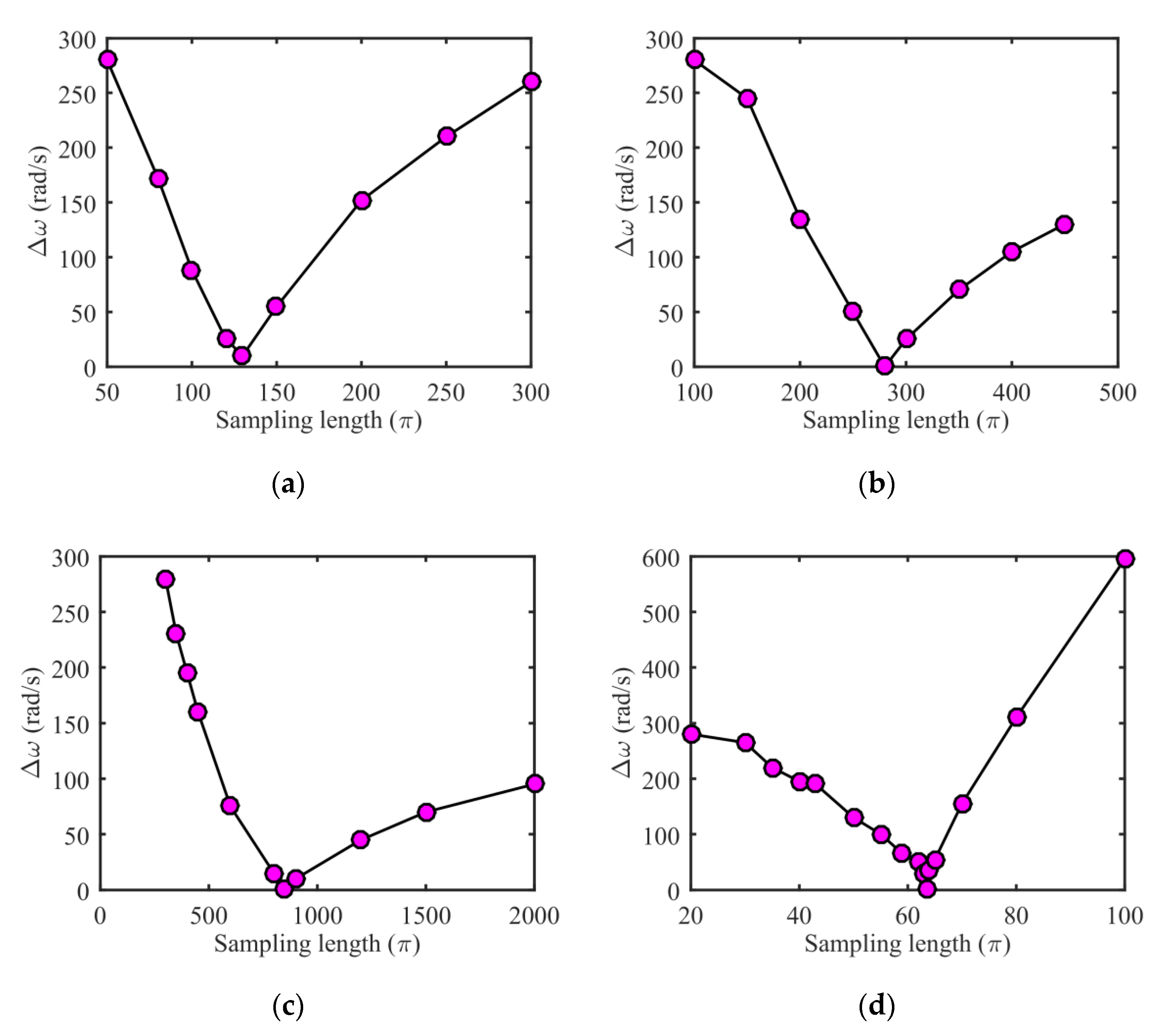
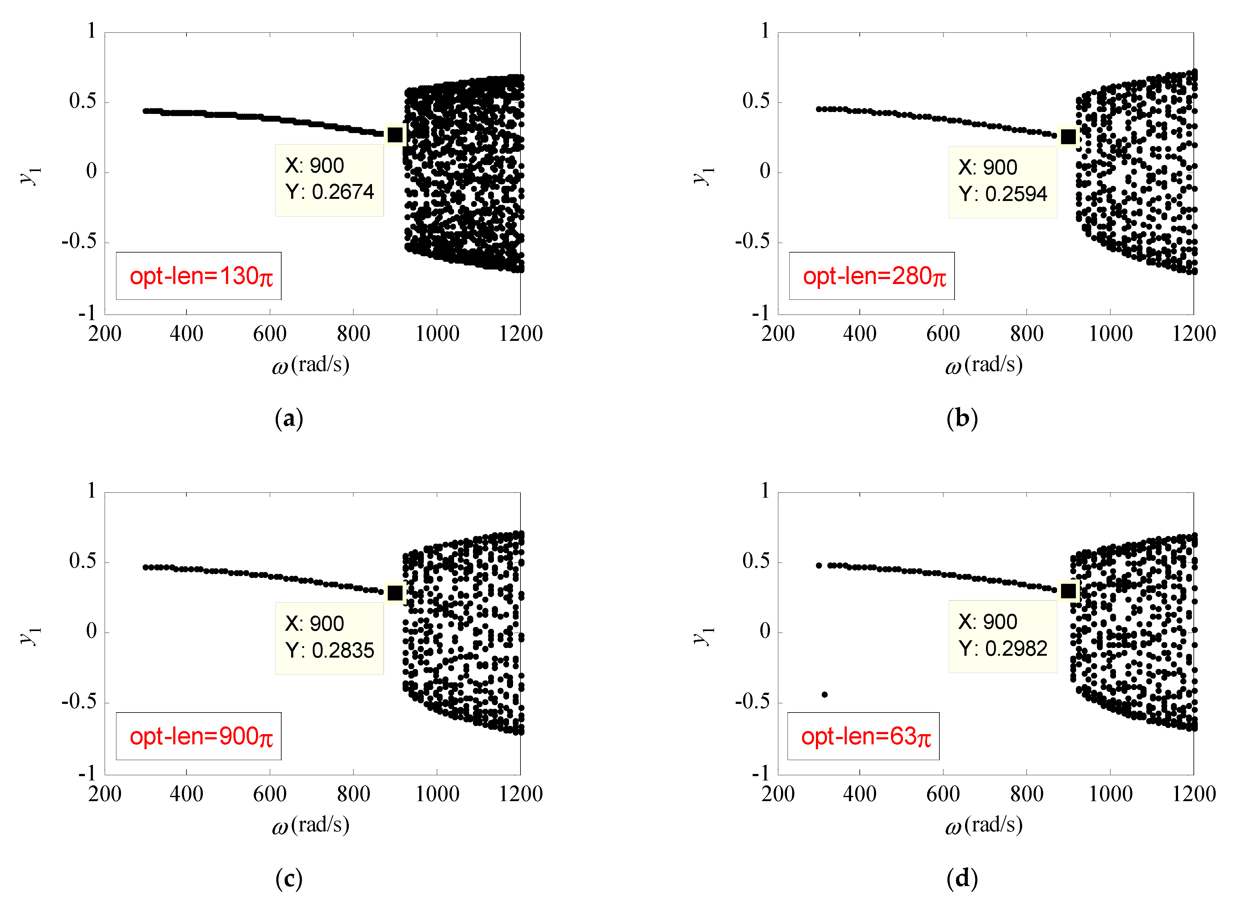
2.2. Order Reduction Model Equivalence of Optimal Sampling Length

The responses and POD POMs of the original system vary with different parameters, so the optimal sampling length is different. For clarity, we use parameter $\omega$ to stand for parameter $\mathit{\alpha }$ in this section. We will discuss the relation of order reduction models obtained by optimal sampling length in different parameters. For two different parameters ${\omega }_1,{\omega }_2\in \left[{\omega }_{\alpha },{\omega }_{\beta }\right]$ in the parameter domain of the high-dimensional complex system (the dimension is n), the corresponding optimal sampling lengths are $t_{opt}^1$, $t_{opt}^2$. The two order reduction models are equivalent when $E_m^1(t,{\mathit{x}}_0,{\omega }_1,t_{opt}^1)$, $E_m^2(t,{\mathit{x}}_0,{\omega }_2,t_{opt}^2)$ are sufficiently small, $S_1,S_2\in S_r$, $S_1\cong S_2$ $X({\mathit{x}}_0,{\omega }_1,t_{opt}^1,t,\omega )\approx X({\mathit{x}}_0,{\omega }_2,t_{opt}^2,t,\omega )\approx X({\mathit{x}}_0,t,\omega )$. Let us prove it briefly as follows.

Let the optimal sampling lengths of two different parameters be ${\omega }_1,{\omega }_2$ are $t_{opt}^1$, and $t_{opt}^2$, $E_m^1(t,{\mathit{x}}_0,{\omega }_1,t_{opt}^1)$, and $E_m^2(t,{\mathit{x}}_0,{\omega }_2,t_{opt}^2)$ are small enough, thus there exists a small $\epsilon >0$, such that

$$E_m^1(t,{\mathit{x}}_0,{\omega }_1,t_{opt}^1)<\frac{\epsilon }{2},E_m^2(t,{\mathit{x}}_0,{\omega }_2,t_{opt}^2)<\frac{\epsilon }{2}.$$

(21)

Equations (22) and (23) can be obtained by Equations (18) and (19)

$$\begin{array}{l}{E}_m^1(t,{\mathit{x}}_0,{\omega }_1,t_{opt}^1)={\displaystyle {\mathsf{\int }}_{{\omega }_{\alpha }}^{{\omega }_{\beta }}{\epsilon }_m^1\left(t,\omega ,\mathit{\phi }({\mathit{x}}_0,{\omega }_1,t_{opt}^1)\right)d\omega }\\ ={\displaystyle {\mathsf{\int }}_{{\omega }_{\alpha }}^{{\omega }_{\beta }}\langle {\Vert X\left({\mathit{x}}_0,t,\omega \right)-{\displaystyle \sum _{i=1}^m{\alpha }_i\left(t,\omega \right){\mathit{\phi }}_i({\mathit{x}}_0,{\omega }_1,t_{opt}^1)}\Vert }^2\rangle d\omega }<\frac{\epsilon }{2}\end{array}$$

(22)

$$\begin{array}{l}{E}_m^2(t,{\mathit{x}}_0,{\omega }_2,t_{opt}^2)={\displaystyle {\mathsf{\int }}_{{\omega }_{\alpha }}^{{\omega }_{\beta }}{\epsilon }_m^2\left(t,\omega ,\mathit{\phi }({\mathit{x}}_0,{\omega }_2,t_{opt}^2)\right)d\omega .}\\ ={\displaystyle {\mathsf{\int }}_{{\omega }_{\alpha }}^{{\omega }_{\beta }}\langle {\Vert X\left({\mathit{x}}_0,t,\omega \right)-{\displaystyle \sum _{i=1}^m{\beta }_i\left(t,\omega \right){\mathit{\phi }}_i({\mathit{x}}_0,{\omega }_2,t_{opt}^2)}\Vert }^2\rangle d\omega }<\frac{\epsilon }{2}\end{array}$$

(23)

Due to Equations (24a) and (24b)

$${\Vert X\left({\mathit{x}}_0,t,\omega \right)-{\displaystyle \sum _{i=1}^m{\alpha }_i\left(t,\omega \right){\mathit{\phi }}_i({\mathit{x}}_0,{\omega }_1,t_{opt}^1)}\Vert }^2\ge 0$$

(24a)

$${\Vert X\left({\mathit{x}}_0,t,\omega \right)-{\displaystyle \sum _{i=1}^m{\beta }_i\left(t,\omega \right){\mathit{\phi }}_i({\mathit{x}}_0,{\omega }_2,t_{opt}^2)}\Vert }^2\ge 0$$

(24b)

so ${\epsilon }_m^1\left(t,\omega ,\mathit{\phi }({\mathit{x}}_0,{\omega }_1,t_{opt}^1)\right)$ and ${\epsilon }_m^2\left(t,\omega ,\mathit{\phi }({\mathit{x}}_0,{\omega }_2,t_{opt}^2)\right)$ are almost everywhere in the parameter domain $\left[{\omega }_{\alpha },{\omega }_{\beta }\right]$, the average TEF of the two parameters is a zero measure set in the parameter domain, ${\epsilon }_m^1\left(t,\omega ,\mathit{\phi }({\mathit{x}}_0,{\omega }_1,t_{opt}^1)\right)$ and ${\epsilon }_m^2\left(t,\omega ,\mathit{\phi }({\mathit{x}}_0,{\omega }_2,t_{opt}^2)\right)$ construct equivalent relation, so $X\left({\mathit{x}}_0,t,\omega \right)$ almost equals to ${\displaystyle \sum _{i=1}^m{u}_i^1\left(t,\omega \right){\mathit{\phi }}_i({\mathit{x}}_0,{\omega }_1,t_{opt}^1)}$ in the parameter domain, meanwhile, as it almost equals to ${\displaystyle \sum _{i=1}^m{u}_i^2\left(t,\omega \right){\mathit{\phi }}_i({\mathit{x}}_0,{\omega }_2,t_{opt}^2)}$, it can be obtained by the following formula

$$\begin{array}{l}{\displaystyle {\mathsf{\int }}_{{\omega }_{\alpha }}^{{\omega }_{\beta }}\langle {\Vert X\left({\mathit{x}}_0,{\omega }_1,t_{opt}^1,t,\omega \right)-X\left({\mathit{x}}_0,{\omega }_2,t_{opt}^2,t,\omega \right)\Vert }^2\rangle d\omega }={\displaystyle {\mathsf{\int }}_{{\omega }_{\alpha }}^{{\omega }_{\beta }}\langle {\Vert {\displaystyle \sum _{i=1}^m{\alpha }_i\left(t,\omega \right){\mathit{\phi }}_i\left({\mathit{x}}_0,{\omega }_1,t_{opt}^1\right)}-{\displaystyle \sum _{i=1}^m{\beta }_i\left(t,\omega \right){\mathit{\phi }}_i\left({\mathit{x}}_0,{\omega }_2,t_{opt}^2\right)}\Vert }^2\rangle d\omega }\\ ={\displaystyle {\mathsf{\int }}_{{\omega }_{\alpha }}^{{\omega }_{\beta }}\langle {\Vert \left(X\left({\mathit{x}}_0,t,\omega \right)-{\displaystyle \sum _{i=1}^m{\beta }_i\left(t,\omega \right){\mathit{\phi }}_i\left({\mathit{x}}_0,{\omega }_2,t_{opt}^2\right)}\right)-\left(X\left({\mathit{x}}_0,t,\omega \right)-{\displaystyle \sum _{i=1}^m{\alpha }_i\left(t,\omega \right){\mathit{\phi }}_i\left({\mathit{x}}_0,{\omega }_1,t_{opt}^1\right)}\right)\Vert }^2\rangle d\omega }\\ \le {\displaystyle {\mathsf{\int }}_{{\omega }_{\alpha }}^{{\omega }_{\beta }}\langle {\Vert X\left({\mathit{x}}_0,t,\omega \right)-{\displaystyle \sum _{i=1}^m{\alpha }_i\left(t,\omega \right){\mathit{\phi }}_i\left({\mathit{x}}_0,{\omega }_1,t_{opt}^1\right)}\Vert }^2\rangle d\omega }+{\displaystyle {\mathsf{\int }}_{{\omega }_{\alpha }}^{{\omega }_{\beta }}\langle {\Vert X\left({\mathit{x}}_0,t,\omega \right)-{\displaystyle \sum _{i=1}^m{\beta }_i\left(t,\omega \right){\mathit{\phi }}_i\left({\mathit{x}}_0,{\omega }_2,t_{opt}^2\right)}\Vert }^2\rangle d\omega }\\ \le \frac{\epsilon }{2}+\frac{\epsilon }{2}\le \epsilon \end{array}$$

(25)

Further

$$X({\mathit{x}}_0,{\omega }_1,t_{opt}^1,t,\omega )\approx X({\mathit{x}}_0,{\omega }_2,t_{opt}^2,t,\omega )\approx X({\mathit{x}}_0,t,\omega ).$$

(26)

Therefore, the order reduction models obtained from the optimal sampling lengths of different sampling parameters constitute equivalent relations when the total average TEF is sufficiently small; that is, the order reduction models are equivalent to each other. In the same way, it can be proved that all order reduction models are equivalent to each other if total average TEF is small enough.

The bifurcation behavior relation of the reduced and original models is discussed if the conditions meet parameter domain order reduction. Assume that the original system only bifurcates once in a parameter domain $\omega \in \left[{\omega }_{\alpha },{\omega }_{\beta }\right]$, the bifurcation points of the original and reduced systems are ${\omega }_c$ and ${\omega }_{c_r}$, respectively, and the bifurcation type of the original system remains the same under the linear transformation of POD POM. Define $\mathsf{\Delta }\omega =\left|{\omega }_{c_r}-{\omega }_c\right|$ as the relative error of the bifurcation parameter, representing the relative distance between the bifurcation point of the reduced and original systems in the parameter domain. $\mathsf{\Delta }\omega \to 0$ means that bifurcations of the reduced and original systems occur on the same or similar parameters, and the bifurcation behaviors of the original and reduced systems are the same in the parameter domain, so the dynamic behaviors are consistent. When the difference of $\mathsf{\Delta }\omega$ is large, assume $\mathsf{\Delta }\omega =\delta$, ${\omega }_{c_r}>{\omega }_c$, so the response behaviors of the reduced and original systems are different in the domain $\omega \in \left[{\omega }_c,{\omega }_{c_r}\right]$, and the response errors of the reduced and original systems are large in the parameter domain, so the order reduction conditions are not satisfied in the entire parameter domain $\omega \in \left[{\omega }_{\alpha },{\omega }_{\beta }\right]$, $E_m^{}(t,{\mathit{x}}_0,{\omega }_s,t_s^{})\gg \epsilon$. Therefore, in order to realize order reduction in the parameter domain of a high-dimensional system, it is necessary to ensure that the relative error of the bifurcation parameters between the reduced and the original systems tend to zero, which is a necessary condition for order reduction in the parameter domain. It can be seen from the above proof that order reduction in the parameter domain can be realized through the optimal sampling length, so the minimum relative error of bifurcation parameters correspond to the optimal sampling length.

Remark 1.

While the total average TEF is different as the system parameters, initial condition, different sampling length and POM number vary, the obtained order reduction models are also different. However, under the condition that the total average TEF is small enough, all the order reduction models are equivalent to each other and can approximately reflect the dynamic behaviors of the original system in the parameter domain. Therefore, order reduction in the parameter domain of high-dimensional complex systems can be realized through the POD POM obtained under these sampling parameters. The POD POM can be constructed by the response signal of optimal sampling length containing transient progress of the system when the system parameters, initial condition, and POM number are confirmed. The invariable order reduction model in the parameter domain of the system is obtained, so as to realize the theoretical research on the high-dimensional complex system, and the order reduction model satisfying the order reduction in the parameter domain has the characteristic that the relative error of bifurcation parameters tends to zero with the original system.

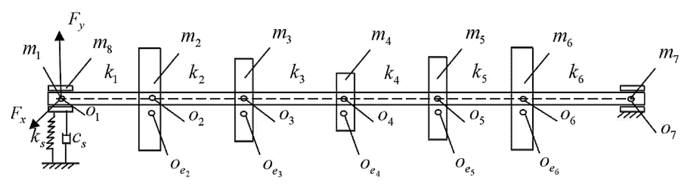
3. Modeling of Rotor-Bearing System with Looseness Fault

In this section, order reduction of the parameter domain for high-dimensional nonlinear rotor system supported by sliding bearing in a certain speed will be studied. The effects of the system parameters, initial condition, sampling length, and mode number to order reduction of the parameter domain will be analyzed, and the POD POMs are confirmed, obtaining invariable order reduction model in parameter domain.

Figure 1 shows the schematic diagram of high-dimensional nonlinear rotor-bearing system model, the rotor contains five impeller discs, it is assumed that each disc is rigid and both ends of the rotor are supported by sliding bearings, and the looseness of the left bearing is considered. Similarly, it is assumed that each shaft section is the elastic shaft section designed with equal stiffness and the geometric center of the left journal, each disc shaft section, and the right journal are $O_i\left(i=1\dots 7\right)$, respectively; the mass of the left and right journals are concentrated in the corresponding geometric center $O_1,O_7$, the mass of other shaft sections are concentrated at the center of mass of each wheel, $O_i{}^{\prime }\left(i=2\dots 6\right)$, the corresponding eccentricity is $e_i\left(i=2\dots 6\right)$; the rotor structure is symmetrical, the gyroscopic of each disc is ignored; selecting the geometric center of the bearing at the left end as the reference point, $x_i,y_i\left(i=1\dots 7\right)$ are the horizontal and vertical displacements of the center of mass of the left journal, the center of mass of each disc, and the right journal relative to the reference point in the radial surface; $m_i,c_i\left(i=1\dots 7\right)$, $k_i\left(i=1\dots 6\right)$ represent equivalent mass, damping. and stiffness of each shaft section of the corresponding positions; $F_x,F_y$ denote the oil film forces in the horizontal and vertical directions. Assume that the looseness of the left end only occurs in the vertical direction, $y_8$ is the displacement of relative reference point, looseness stiffness $k_s$ and damping $c_s$ are piecewise linear functions [20,21,22].

$$k_s=\{\begin{array}{l}{k}_s^1(y_8>\delta )\\ 0(0\le y_8\le \delta )\\ k_s^2(y_8<0)\end{array},c_s=\{\begin{array}{l}{c}_s^1(y_8>\delta )\\ 0(0\le y_8\le \delta )\\ c_s^2(y_8<0)\end{array}.$$

(27)

Consider the nonlinear oil film force of the bearing at both ends and the unbalanced excitation of the rotor, the motion differential equation of the multidisc rotor-bearing system can be established by the Newton’s second law, the dynamical equation can be expressed as Equation (1). where $X={\left[x_1,\dots ,x_7,y_1\dots y_7,y_8\right]}^T$, M, C, and K are stiffness, mass, and damping matrices, which can be expressed as:

$$M=\left[\begin{array}{cc}\begin{array}{ccc}{m}_1& & \\ & \ddots & \\ & & m_7\end{array}& 0\\ 0& \begin{array}{cccc}{m}_1& & & \\ & \ddots & & \\ & & m_7& \\ & & & m_8\end{array}\end{array}\right],C=\left[\begin{array}{cc}\begin{array}{ccc}{c}_1& & \\ & \ddots & \\ & & c_7\end{array}& 0\\ 0& \begin{array}{cccc}{c}_1& & & \\ & \ddots & & \\ & & c_7& \\ & & & c_s\end{array}\end{array}\right]$$

(28a)

$$K=\left[\begin{array}{cc}\begin{array}{cccccc}{k}_1& -k_1& & & & \\ -k_1& k_1+k_2& -k_2& & & \\ & -k_2& \ddots & \ddots & & \\ & & \ddots & k_4+k_5& -k_5& \\ & & & -k_5& k_5+k_6& -k_5\\ & & & & -k_5& k_6\end{array}& 0\\ 0& \begin{array}{cccccc}{k}_1& -k_1& & & & \\ -k_1& k_1+k_2& -k_2& & & \\ & -k_2& \ddots & \ddots & & \\ & & \ddots & k_4+k_5& -k_5& \\ & & & -k_5& k_5+k_6& -k_5\\ & & & & -k_5& k_6\end{array}\begin{array}{c}\\ \\ \\ \\ \\ \\ k_s\end{array}\end{array}\right]$$

(28b)

$F\left(X,\dot{X},t\right)$ represents the external force vector, including the nonlinear oil force of the left and right journal, eccentric excitation of each disc and gravity, the expression is shown as:

$$\begin{array}{l}F=[F_X(x_1,y_1-y_8,{\dot{x}}_1,{\dot{y}}_1-{\dot{y}}_8),m_2{e}_2{\omega }^2\cos (\omega t),\dots ,m_6{e}_6{\omega }^2\cos (\omega t),F_X(x_7,y_7,{\dot{x}}_7,{\dot{y}}_7),F_Y(x_1,y_1-y_8,{\dot{x}}_1,{\dot{y}}_1-{\dot{y}}_8)-m_{1}g,\\ m_2{e}_2{\omega }^2\sin (\omega t)-m_{2}g,\dots ,m_6{e}_6{\omega }^2\sin (\omega t)-m_{6}g,F_Y(x_7,y_7,{\dot{x}}_7,{\dot{y}}_7)-m_{7}g,-F_Y(x_1,y_1-y_8,{\dot{x}}_1,{\dot{y}}_1-{\dot{y}}_8)-m_{8}g{]}^T\end{array}$$

(29)

For the convenience of analysis, the dimensionless process is shown as follows:

$$\begin{array}{l}\tau =\omega t,x_i=\frac{X_i}{c},y_i=\frac{Y_i}{c},M_1=\frac{m_{1}c{\omega }^2}{sW},M_7=\frac{m_{7}c{\omega }^2}{sW},M_8=\frac{m_{8}c{\omega }^2}{sW},\\ e_i^{\prime }=\frac{e_i}{c}(i=2\dots 6),f_x=\frac{F_X}{sW},f_y=\frac{F_Y}{sW},\\ \left\{\begin{array}{l}{f}_x\\ f_y\end{array}\right\}=-\frac{\sqrt{{\left(x-2\dot{y}\right)}^2+{\left(y+2\dot{x}\right)}^2}}{1-x^2-y^2}\left\{\begin{array}{l}3xV\left(x,y,\alpha \right)-\sin \alpha G\left(x,y,\alpha \right)-2\cos \alpha S\left(x,y,\alpha \right)\\ 3yV\left(x,y,\alpha \right)+\cos \alpha G\left(x,y,\alpha \right)-2\sin \alpha S\left(x,y,\alpha \right)\end{array}\right\},\\ \alpha =\arctan \left(\frac{y+2\dot{x}}{x-2\dot{y}}\right)-\frac{\pi }{2}sign\left(\frac{y+2\dot{x}}{x-2\dot{y}}\right)-\frac{\pi }{2}sign\left(y+2\dot{x}\right),\\ G\left(x,y,\alpha \right)=\frac{2}{\sqrt{1-x^2-y^2}}\left[\frac{\pi }{2}+\arctan \left(\frac{y\cos \alpha -x\sin \alpha }{\sqrt{1-x^2-y^2}}\right)\right],\\ V\left(x,y,\alpha \right)=\frac{2+\left(y\cos \alpha -x\sin \alpha \right)G\left(x,y,\alpha \right)}{1-x^2-y^2},\\ S\left(x,y,\alpha \right)=\frac{x\cos \alpha +y\sin \alpha }{1-{\left(x\cos \alpha +y\sin \alpha \right)}^2}\end{array}$$

(30)

where $f_x,f_y$ are nonlinear oil film forces in two perpendicular directions, respectively; $s=\frac{\mu \omega RL}{W}{(\frac{R}{c})}^2{(\frac{L}{2R})}^2$ is Sommerfeld coefficient [23]; $\omega$ is angular frequency; $\mu$ is coefficient of viscosity; $R$, $L$ and $W$ represent radius, length, and half weight of the rotor system, respectively. The system parameters shown in

Table 1. Parameters of the rotor-bearing system.

Parameter	Value	Parameter	Value
m1 = m7 (kg)	4	c1 = c7 (N.s/m)	800
m2 = m6 (kg)	25	c2 =c6 (N.s/m)	1750
m3 = m5 (kg)	20	c3 =c5(N.s/m)	1550
m4 (kg)	10	c4(N.s/m)	1350
m8 (kg)	5	$c_s^1$(N.s/m)	350
ki (i = 1…6) (N/m)	5 × 108	$c_s^2$(N.s/m)	500
$k_s^1$ (N/m)	2.5 × 108	$\delta$(mm)	0.22
$k_s^2$ (N/m)	1 × 109	L (mm)	30
e3 (mm)	0.01	R (mm)	30
$\mu$ (pa.s)	0.018	c (mm)	0.11
m1 = m7(kg)	4	c1 = c7 (N.s/m)	800

.

The fourth order Runge-Kutta method is used to calculate the response of 15-DOF original system, the displacement response signals $\widehat{X}\left({\mathit{x}}_0,\omega ,t_s\right)={[x_1,\dots ,x_7,y_1,\dots ,y_7,y_8]}_{N_s\times 15}$ of different parameters are extracted, as a sampling snapshot matrix, where ${\mathit{x}}_0,\omega ,t_s$ represent the initial conditions, speed, and sampling length (N_s is data length) of the sampling signal. Since the transient motion contains free and forced vibration, and contains the inherent mode information of the system, each parameter sampling contains transient motion of the system. By calculating the eigenvectors of the autocorrelation matrix

$$S_c=\frac{1}{N_s}{[\widehat{X}{\left({\mathit{x}}_0,\omega ,t_s\right)}^T\widehat{X}\left({\mathit{x}}_0,\omega ,t_s\right)]}_{15\times 15}$$

(31)

the eigenvectors are arranged in descending order of eigenvalues and the POD POM ${\left\{{\mathit{\phi }}_i\left({\mathit{x}}_0,\omega ,t_s\right)\right\}}_{i=1\dots 15}$ can be obtained. The original system is projected onto the subspace spanned by the first m order POMs, that is, the following coordinate transformation relation is obtained

$$X(t)={\displaystyle \sum _{i=1}^m{u}_i(t)}{\mathit{\phi }}_i\left({\mathit{x}}_0,\omega ,t_s\right)=P\left({\mathit{x}}_0,\omega ,t_s,m\right)\mathit{u}\left(t\right)$$

(32)

where $P\left({\mathit{x}}_0,\omega ,t_s,m\right)={\left[{\mathit{\phi }}_1\left({\mathit{x}}_0,\omega ,t_s\right),\dots ,{\mathit{\phi }}_m\left({\mathit{x}}_0,\omega ,t_s\right)\right]}_{15\times m}$, and the dynamical equation of order reduction model can be obtained by substituting Equation (32) to Equation (1)

$$M_r\ddot{\mathit{u}}+C_r\dot{\mathit{u}}+K_r\mathit{u}=F_r\left(\mathit{u},\dot{\mathit{u}},t\right)$$

(33)

where $M_r=P^{T}MP$, $C_r=P^{T}CP$, $K_r=P^{T}KP$, $F_r=P^{T}F$, the initial condition can be confirmed by ${\mathit{u}}_0=P^T{\mathit{x}}_0$.

$M_r,C_r,K_r,F_r$ of the order reduction model relate to system parameter, initial condition, sampling length, and POM number. However, on the basis of the proof in Section 2, the order reduction models are equivalent to each other when the sampling signal with sufficiently small total average truncation error is satisfied, and the order reduction model is determined once the sampling snapshot signal matrix of the original system is determined. Therefore, the effects of system parameters, initial conditions, sampling length, and POM number on the order reduction in the parameter domain can be analyzed to determine the POM in the parameter domain and obtain the constant order reduction model of the system in the parameter domain. The efficiency of order reduction in parameter domain is verified by numerical method.

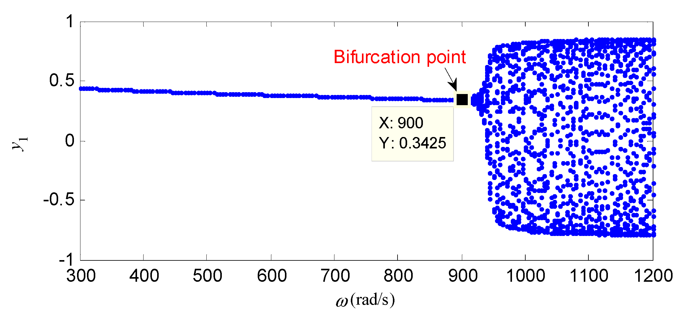
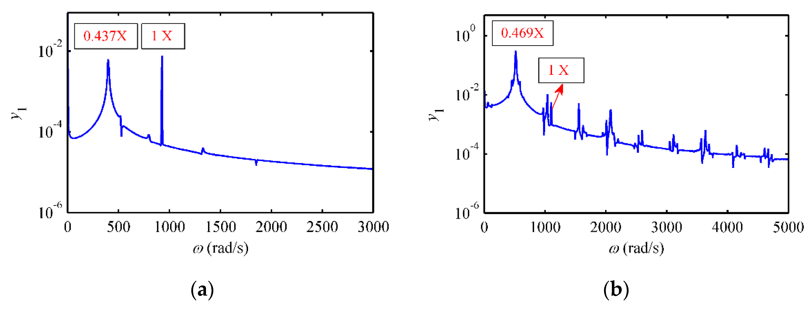
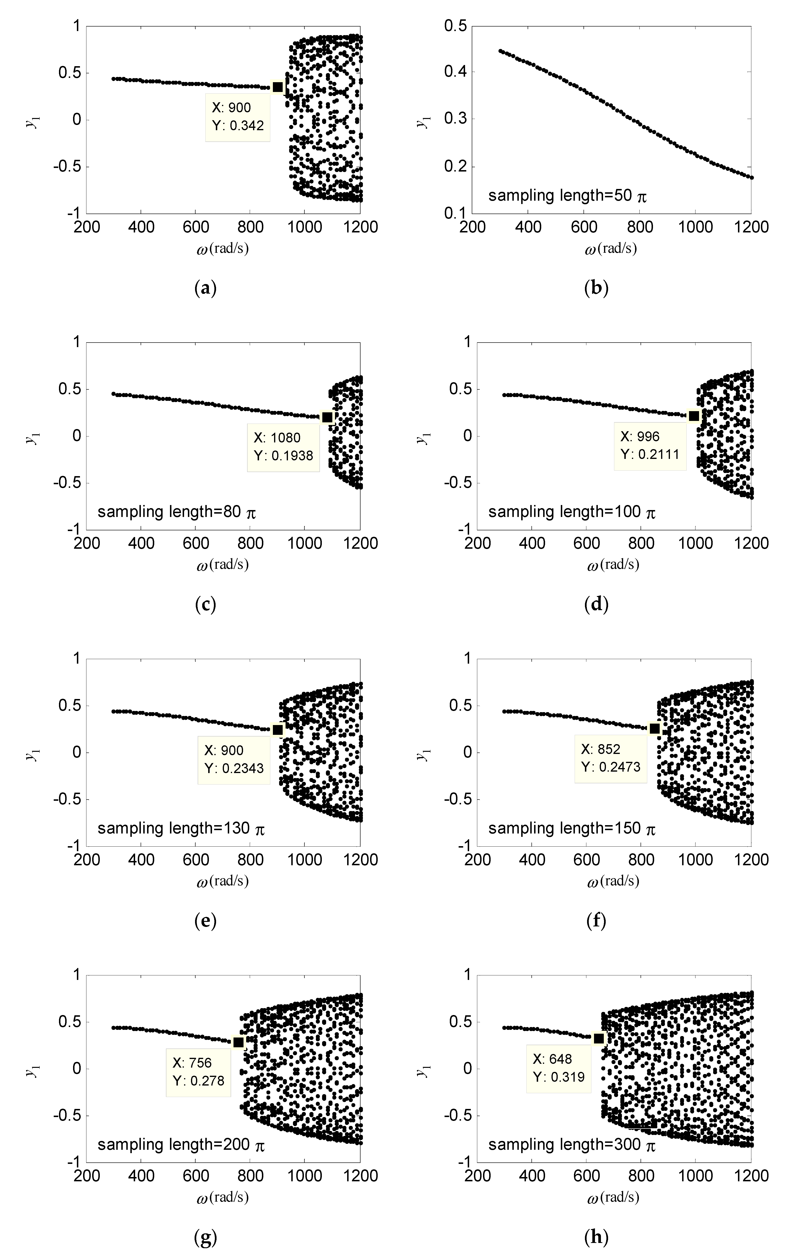
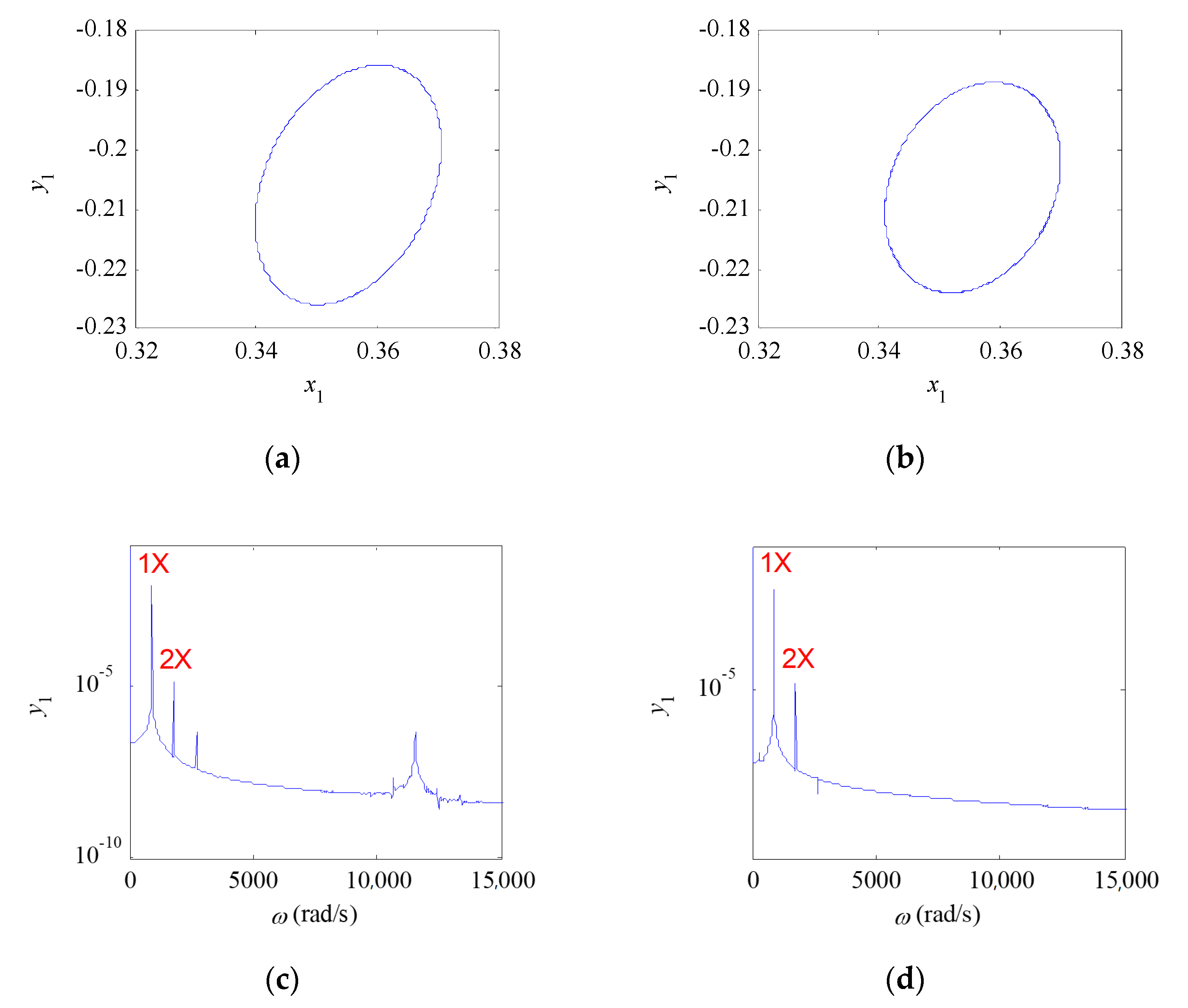
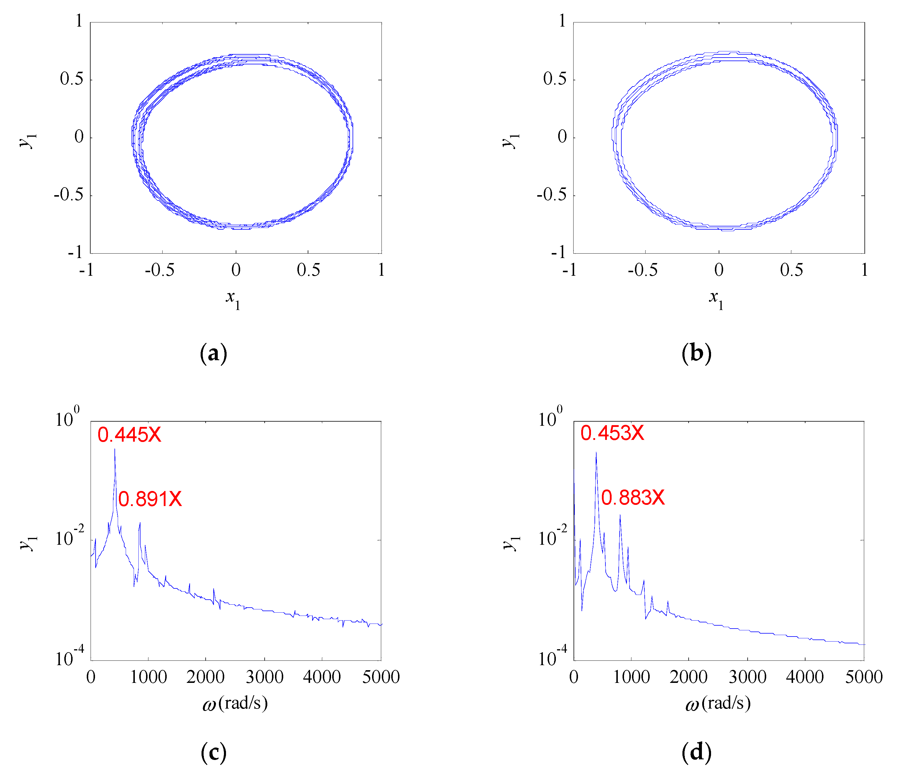
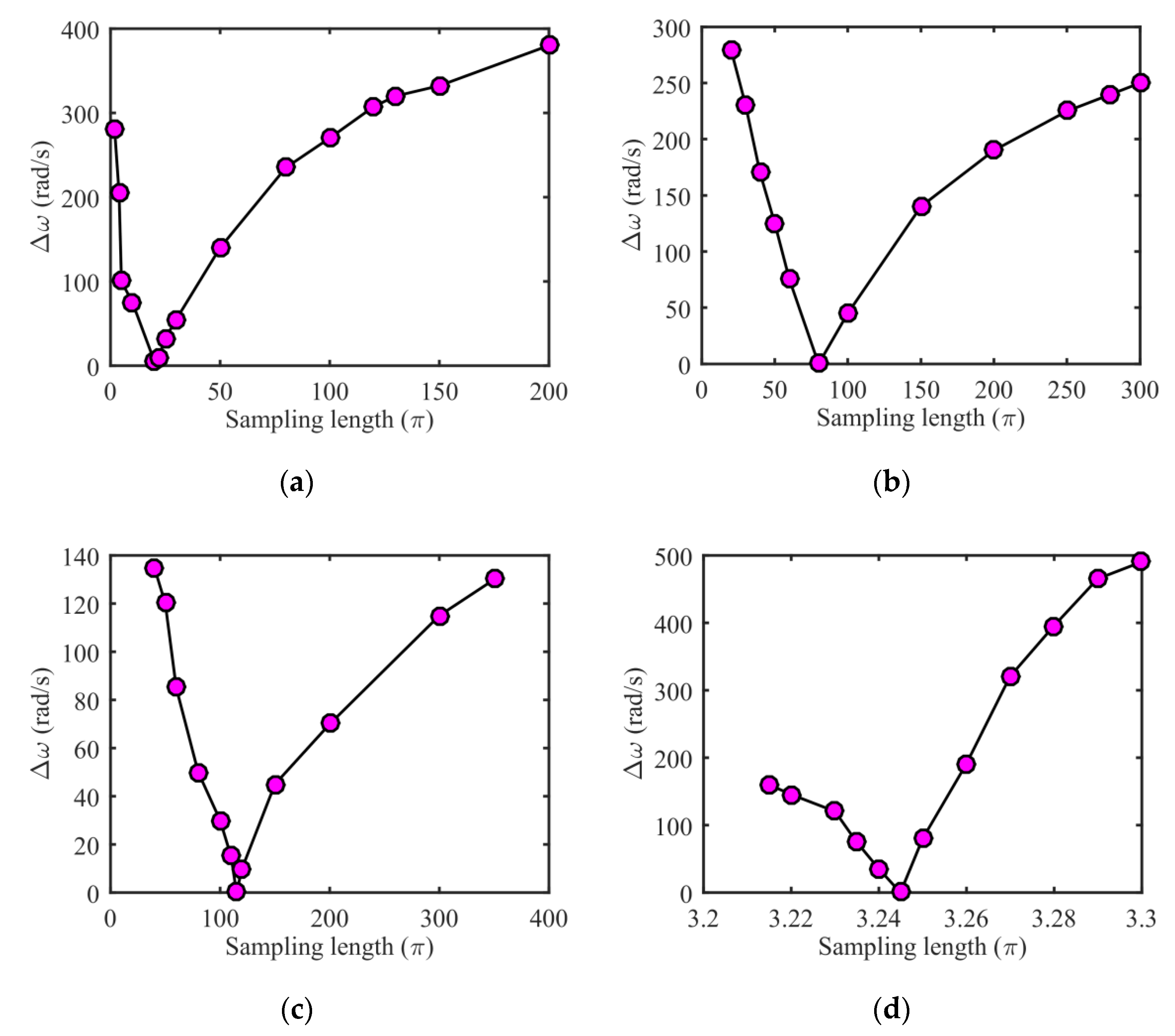
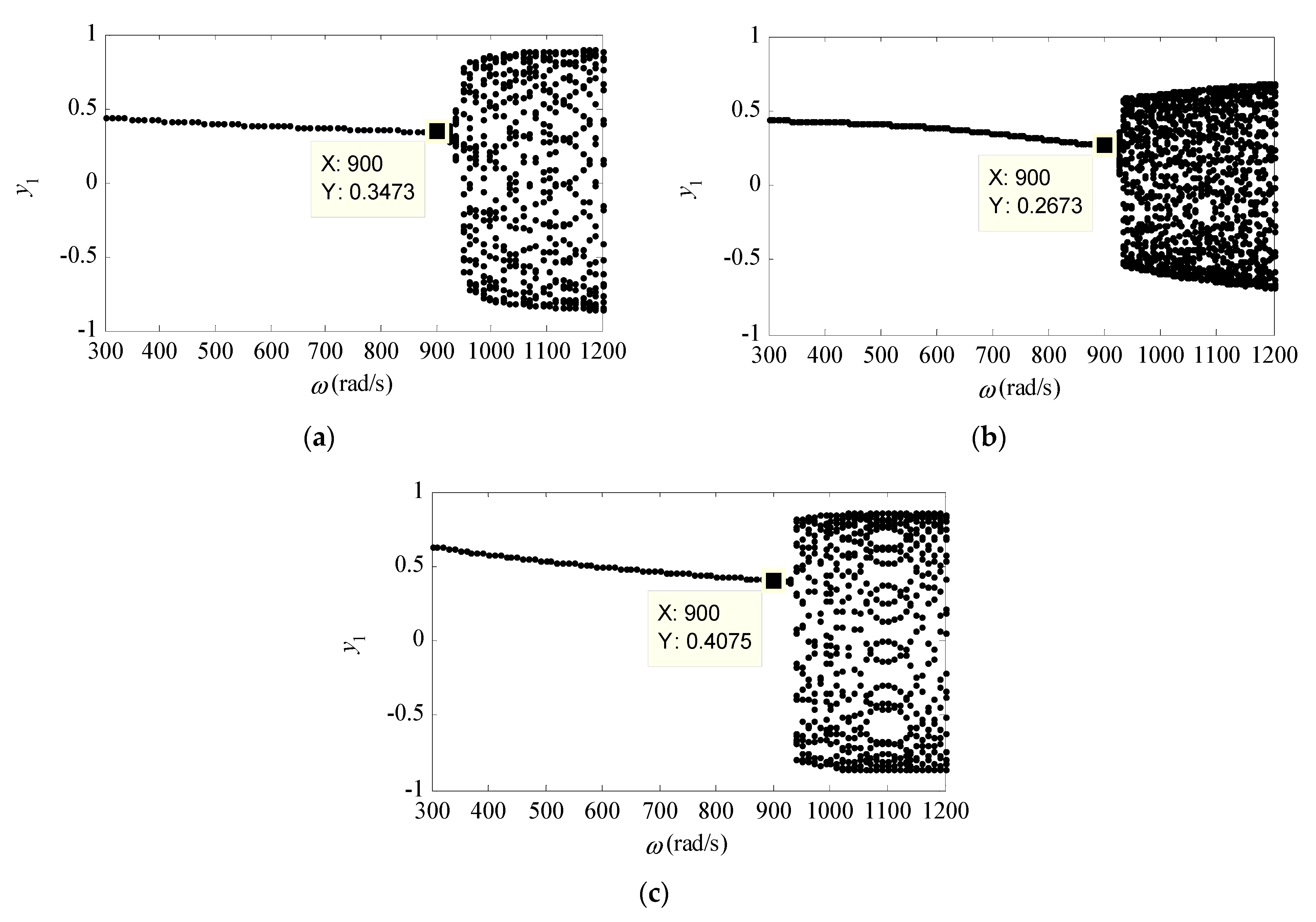
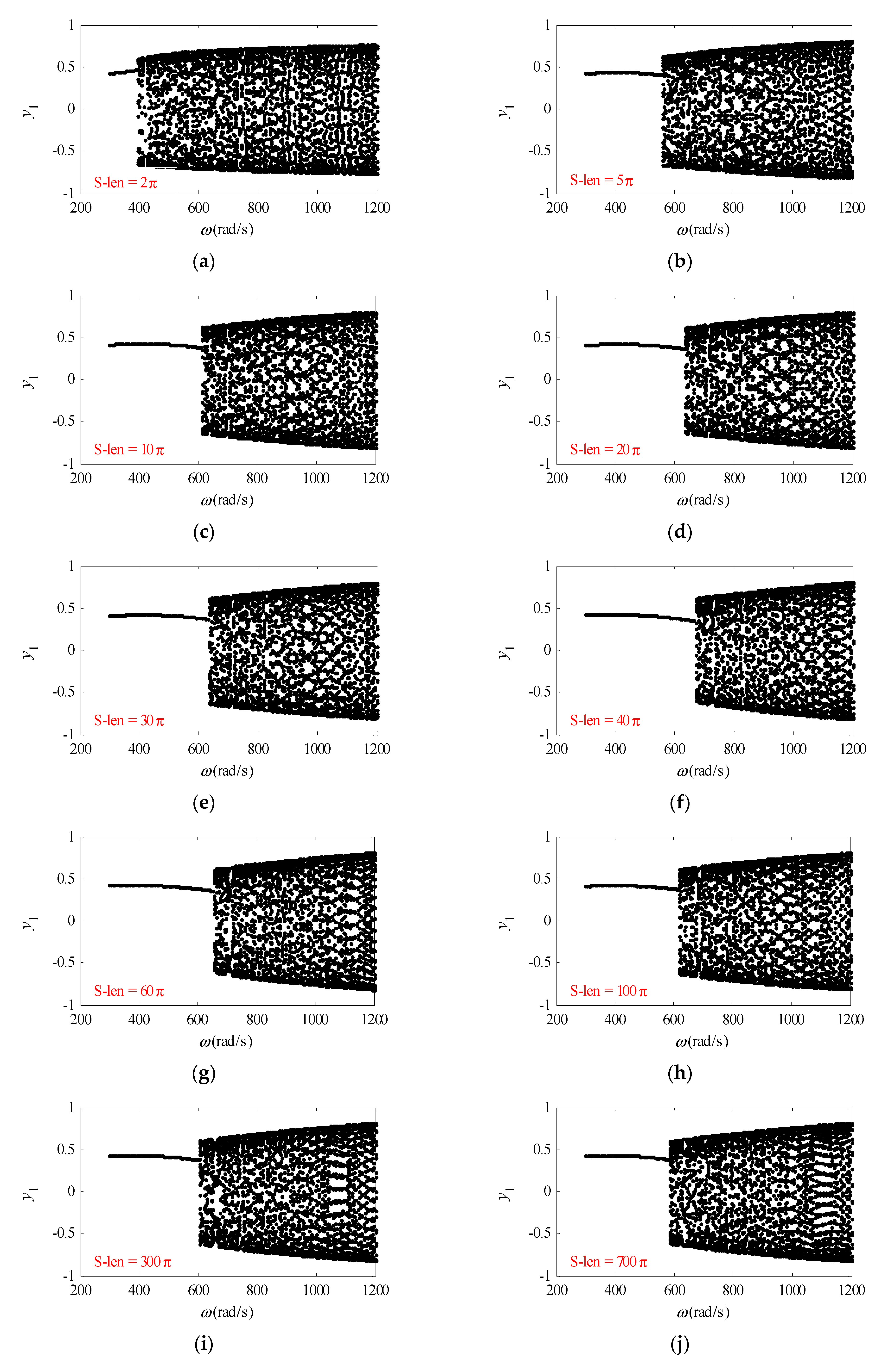
4. Analysis of Dynamics and Order Reduction Efficiency

The numerical results will be discussed in this section, including bifurcation behavior analysis, optimal sampling length and order reduction efficiency study of the POD method.

Choose speed as the parameter of order reduction for the system, the speed range is $\left[300,1200\right]$ rad/s, the bifurcation diagram of the original system in the speed range can be obtained by numerical integration, which is shown in Figure 2. It can be seen from the figure that the response of the system bifurcates at ${\omega }_c=915$ rad/s, and at the speed of $\left[300,915\right]$ rad/s, the system is period-1 motion; the complex bifurcation behaviors occur at the speed $\left[915,1200\right]$ rad/s and the vibration is larger in this speed domain—it is an oil film oscillation phenomenon caused by the nonlinear oil film force, its main characteristic is that there is a large peak value in the response spectrum near the half frequency of rotating shaft. As shown in Figure 3, it is the spectrum diagram corresponding to the two rotating speeds in the oil film oscillation region of the original system. At the rotating speed of 915 rad/s, the oil film instability just occurred in the system. When the rotating speed is 1100 rad/s, the frequency component amplitude of the 0.469 times rotating shaft is very large and oil film oscillation of the system occurs violently.

For the parameter domain order reduction, most order reduction models have approximately the same bifurcation behaviors in parameter domain with original model, such as similar bifurcation diagram structure, close bifurcation point, and consistent bifurcation behavior. As usual, we first use a bifurcation diagram structure and then the bifurcation to verify the efficiency of the parameter domain order. Therefore, in order to analyze the effect of sampling parameters on parameter domain order reduction, we mainly compare the bifurcation diagram of the order reduction model with the original system under different sampling conditions.

Firstly, the effects of sampling length on parameter domain order reduction are analyzed. Suppose the initial value of the original system state vector is $x_i=y_i=0.69$, $y_8=0.25$, ${\dot{x}}_i={\dot{y}}_i={\dot{y}}_8=0\left(i=1\dots 7\right)$, the response signals of the original system at different time lengths are obtained at a fixed speed, and the order reduction model at the corresponding sampling length is obtained. The bifurcation behaviors of the original system were compared in the range of speed [300,1200] rad/s. In Figure 4, it is a bifurcation diagram of the original system and a bifurcation diagram of two-DOF reduction models obtained at different sampling lengths with sampling speed 350 rad/s. As can be seen from the figure, the bifurcation points of the order reduction models with sampling lengths of $50\pi ,80\pi ,100\pi ,130\pi ,150\pi ,200\pi ,300\pi$ are 1200 rad/s, 1100 rad/s, 1005 rad/s, 910 rad/s, 865 rad/s, 775 rad/s, 655 rad/s respectively. As the sampling length increases, the bifurcation point of the order reduction model gradually decreases until it converges. Compared with the bifurcation diagram of the original system, it is easy to find that only when the sampling length is 130π, does the bifurcation diagram of the order reduction model have a similar structure to the original system, where the bifurcation points are closest to each other in the rotation speed domain and have the smallest error with the original system; however, the order reduction models at other sampling lengths greatly differ from the bifurcation diagram structure of the original system, and the bifurcation points are far away in the speed domain. It can be seen that the two-DOF order reduction model obtained at this sampling length can depict the bifurcation characteristics of the original system with 15-DOF in the parameter domain, while the order reduction models at other sampling lengths cannot reflect the bifurcation behaviors of the original system. Therefore, the sampling length can be considered as the optimal sampling length with a sampling speed of 350 rad/s and a POM number of 2.

Figure 5 and Figure 6 are the orbit of shaft center and spectrum diagrams of the two-DOF order reduction model at the sampling speed of 350 rad/s and the optimal sampling length at the speeds of 900 rad/s and 950 rad/s, as well as orbit of shaft center and spectrum diagrams of the corresponding speed of the original system. As can be seen from the figure, the orbit of shaft center and spectrum of the order reduction model are basically similar to the original system, at speed of 900 rad/s, the period of both is 1; at speed of 950 rad/s, both are almost periodic motions. The main frequency of the original system and the order reduction model are 0.445 times and 0.453 times the shaft frequency, respectively, which is about half the shaft frequency. The amplitude of the shaft frequency component is weak. These characteristics are consistent with oil film oscillation phenomenon of the original system. The oil film oscillation region of the order reduction model is consistent with the original system. Therefore, the two-DOF invariant order reduction model obtained from the optimal sampling length of 350 rad/s can reflect the main dynamic behaviors of the original system in the parameter domain and can realize the order reduction of the system on parameter domain.

Without loss of generality, we also sampled at other speeds to analyze the similarity between the order reduction model obtained from different sampling lengths and the bifurcation diagram of the original system. Here, we express the relationship between the relative error of the bifurcation parameters and the sampling length. Figure 7 shows the relationship between the sampling length and the relative error of the bifurcation parameter of the two-DOF order reduction model obtained at four different sampling speeds (350 rad/s, 500 rad/s, 700 rad/s, 1000 rad/s) and different sampling lengths. As can be seen from the four subgraphs in Figure 7, there is a sampling length at each sampling speed that makes the relative error of the bifurcation parameter zero or close to zero. The order reduction model obtained by this sampling length is similar to the bifurcation diagram structure of the original system, and the bifurcation occurs on the same or similar parameters in the parameter domain. However, the bifurcation diagram structure of order reduction model obtained far from this sampling length keeps large differences of the original system, and the bifurcation occurs on different parameters in the parameter domain. Therefore, the relative error of the bifurcation parameter in each figure is zero or close to zero, which is the optimal sampling length of each speed. Only the order reduction model obtained under the optimal sampling length has similar dynamic behaviors with the original system in the parameter domain. As can be seen from the figure, the optimal sampling lengths corresponding to the four sampling speeds are $130\pi ,280\pi ,900\pi ,63\pi$, respectively. Therefore, when sampling in the simple motion speed domain of the system, the optimal sampling length increases as the sampling speed increases; in the unstable region, the optimal sampling length is relatively small, and the relative error of the bifurcation parameter is sensitive to the variation of the sampling length.

Figure 8 is a bifurcation diagram of a two-DOF order reduction model obtained at four different sampling speeds (350 rad/s, 500 rad/s, 700 rad/s, 1000 rad/s) in the optimal sampling length. As can be seen from the figure, the structure of the bifurcation diagram of the two-DOF order reduction model obtained by the optimal sampling length at four different sampling speeds is very similar, and the bifurcation points are basically the same. Therefore, the bifurcation behaviors of the four order reduction models in this speed range are consistent, and all of them can reflect the dynamic behaviors of the original system in the parameter domain. The above numerical results are consistent with the theoretical results in Section 2, the order reduction models obtained from the optimal sampling length of different parameters in the parameter domain are equivalent to each other, and the minimum relative error value of bifurcation parameters corresponds to the optimal sampling length.

It can be known from the previous theoretical analysis that the POD POM number also has an effect on the parameter domain order reduction. Therefore, the effect of the POM number on the optimal sampling length is analyzed below. According to the analysis idea of the two-DOF order reduction model, the relationship between the sampling length and the relative error of the bifurcation parameter of the three-DOF order reduction model will be analyzed below. Figure 9 shows the relationship between the sampling length and the relative error of the bifurcation parameters of the three-DOF order reduction model at four different sampling speeds (350 rad/s, 500 rad/s, 700 rad/s, 1000 rad/s) and different sampling lengths. It can be known from each sub-graph that each rotation speed also has a sampling length that makes the relative error of the bifurcation parameter zero or close to zero. The order reduction model obtained by this sampling length is similar to the bifurcation diagram structure of the original system. The bifurcation occurs on the same or similar parameters in the parameter domain. The bifurcation diagram structure of the order reduction model obtained from this sampling length has large differences to the bifurcation diagram structure of the original system. Bifurcations occur on different parameters in the parameter domain. Therefore, there is also an optimal sampling length for each sampling speed of the three-DOF order reduction model. It can be seen from Figure 9a–c that the best sampling lengths for sampling in the simple motion speed range are $20\pi ,80\pi ,115\pi$, the optimal sampling length increases as the sampling speed increases. Sampling in the range of complex motion speeds, the optimal sampling length is relatively short, and the relative error of the bifurcation parameters is also sensitive to variation in sampling length. This conclusion is the same as the two-DOF order reduction model. Comparing Figure 9 with Figure 7, the optimal sampling length of the three-DOF order reduction model is shorter than the optimal sampling length of the two-DOF order reduction model at each sampling speed.

Figure 10 shows the bifurcation diagram of the original system and the bifurcation diagram of the 2-DOF and 3-DOF order reduction model obtained at the sampling speed of 350 rad/s using the optimal sampling length. As can be seen from the figure, the bifurcation diagram of the 3-DOF invariant order reduction model contains a more detailed structure in the parameter domain, which is more similar to the original system bifurcation diagram. However, the existing nonlinear dynamics theory still has difficulties in dealing with nonlinear systems with three or more DOFs. The two-DOF order reduction model that can ensure that its main structure of the bifurcation diagram is similar to the original system, and when the bifurcation occurs on the same or similar parameters, the bifurcation behaviors are the same. Therefore, an invariant order reduction model with two-DOF can be obtained via the optimal sampling length at the sampling speed, and the theoretical analysis to a high-dimensional nonlinear system can be realized.

According to the above analysis, although the optimal sampling length can be used to obtain the invariant order reduction model of the high-dimensional complex system in the parameter domain, only the order reduction model can represent the main vibration behaviors of the original system in the parameter domain under the condition that the total average truncation error is small. It can be known from the previous theoretical analysis that the total average truncation error is related to the system parameters, initial conditions, sampling length, and POM number. Under certain conditions, the optimal sampling length may not meet the condition that the total average truncation error is small. Therefore, even the order reduction model obtained by the optimal sampling length cannot reflect the main dynamic behaviors of the original system in the parameter domain. Figure 11 is the bifurcation diagram of the two-DOF order reduction model with initial conditions as follows: $x_i=y_i=y_8=0.1,{\dot{x}}_i={\dot{y}}_i={\dot{y}}_8=0\left(i=1\dots 7\right)$, rotor speed 500 rad/s, and different sampling lengths. It can be seen from the figure that when the sampling length is less than 40π, as the sampling length increases, the bifurcation area of the order reduction model shrinks, the bifurcation point moves to the right, and it is closer to the original system bifurcation point; when the sampling length is greater than 40π, as the sampling length increases, the bifurcation area of the order reduction model increases, and the bifurcation point moves to the left, far away from the bifurcation point of the original system. In all the sampling lengths, only the bifurcation region of the order reduction model obtained by 40π is closest to the original system, which is the optimal sampling length for this condition. However, the bifurcation area of the order reduction model of the sampling length still has large difference from the original system. Therefore, the optimal sampling length under this initial condition is in the parameter domain, and an invariant order reduction model that can approximately reflect the dynamic behaviors of the original system cannot be obtained.

Remark 2.

The reason why the above initial conditions cannot obtain an invariant order reduction model that can approximately reflect the dynamic behaviors of the original system in the parameter domain can be expressed as: the initial value is too small to stimulate the inherent modal information of the original system during the transient response. Therefore, the dynamic behaviors of the order reduction model obtained under this initial condition differ greatly from the original system in the parameter domain.

5. Conclusions and Outlooks

In the parameter domain, the adaptive POD method cannot obtain a low-dimensional invariant model that can approximately reflect the dynamic behaviors of high-dimensional systems, so in-depth theoretical research is difficult to carry out. This manuscript focused on this problem, proposed the transient POD method based on minimum error of bifurcation parameter, and provided the order reduction conditions of parameter domain. The conclusions are summarized as follows:

• The transient POD method based on minimum error of bifurcation parameter has been proposed, and the order reduction of parameter domain of this method has been provided.
• The equivalence of different order reduction models that satisfy parameter domain order reduction conditions has been proved.
• A rotor system with looseness fault and supported by sliding bearings has been established by the Newton’s second law.
• The effects of speed, initial conditions, sampling length, and POM number to parameter domain order reduction has been analyzed and the existence of the optimal sampling length has been verified.

Future work can be focused on two main directions: one is to apply the transient POD method to large flexible spacecraft [24], the other one is to use the proposed method to study high-dimensional nonlinear rotor-bearing dynamic systems with typical faults [25,26,27] and parametric uncertainties [28,29,30,31].

References

1. Xumin, G.; Jin, Z.; Hui, M.; Chenguang, Z.; Xi, Y.; Bangchun, W. A dynamic model for simulating rubbing between blade and flexible casing. J. Sound Vib. 2020, 466, 115036. [Google Scholar]
2. Fu, C.; Xu, Y.; Yang, Y.; Lu, K.; Gu, F.; Ball, A. Response analysis of an accelerating unbalanced rotating system with both random and interval variables. J. Sound Vib. 2020, 466, 115047. [Google Scholar] [CrossRef]
3. Yongfeng, Y.; Qinyu, W.; Yanlin, W.; Weiyang, Q.; Kuan, L. Dynamic Characteristics of Cracked Uncertain Hollow-shaft. Mech. Syst. Signal Process. 2019, 124, 36–48. [Google Scholar] [CrossRef]
4. Shibo, Z.; Xingmin, R.; Wangqun, D.; Kuan, L.; Yongfeng, Y.; Chao, F. A transient characteristic-based balancing method of rotor system without trail weights. Mech. Syst. Signal Process. 2021, 148, 107117. [Google Scholar]
5. Jin, Z.; Chenguang, Z.; Hui, M.; Kun, Y.; Bangchun, W. Rubbing dynamic characteristics of the blisk-casing system with elastic supports. Aerosp. Sci. Technol. 2019, 95, 105481. [Google Scholar]
6. Yulin, J.; Kuan, L.; Chongxiang, H.; Lei, H.; Yushu, C. Nonlinear dynamic analysis of a complex dual rotor-bearing system based on a novel model reduction method. Appl. Math. Model. 2019, 75, 553–571. [Google Scholar]
7. Marion, M.; Temam, R. Nonlinear Galerkin methods. SIAM J. Numer. Anal. 1989, 26, 1139–1157. [Google Scholar] [CrossRef]
8. Kim, S.M.; Kim, J.G.; Chae, S.W.; Park, K.C. Evaluating mode selection methods for component mode synthesis. AIAA J. 2016, 54, 2852–2863. [Google Scholar] [CrossRef]
9. Willcox, K.; Peraire, J. Balanced model reduction via the proper orthogonal decomposition. AIAA J. 2002, 40, 2323–2330. [Google Scholar] [CrossRef]
10. Kuan, L.; Yulin, J.; Pangfeng, H.; Fan, Z.; Haopeng, Z.; Chao, F.; Yushu, C. The applications of POD method in dual rotor-bearing systems with coupling misalignment. Mech. Syst. Signal Process. 2021, 150, 107236. [Google Scholar]
11. Daniele, D.; Edoardo, F. Modal parameter estimation for a wetted plate under flow excitation: A challenging case in using POD. J. Sound Vibr. 2019, 469, 214–234. [Google Scholar]
12. Rega, G.; Troger, H. Dimension reduction of dynamical systems: Methods, models, applications. Nonlinear Dyn. 2005, 41, 1–15. [Google Scholar] [CrossRef]
13. Steindl, A.; Troger, H. Methods for dimension reduction and their application in nonlinear dynamics. Int. J. Solids Struct. 2001, 38, 2131–2147. [Google Scholar] [CrossRef]
14. Kuan, L.; Yulin, J.; Yushu, C.; Yongfeng, Y.; Lei, H.; Zhiyong, Z.; Zhonggang, L.; Chao, F. Review for order reduction based on proper orthogonal decomposition and outlooks of applications in mechanical systems. Mech. Syst. Signal Process. 2019, 123, 264–297. [Google Scholar]
15. Kerschen, G.; Golinval, J.C.; Vakakis, A.F.; Bergman, L.A. The method of proper orthogonal decomposition for dynamical characterization and order reduction of mechanical systems: An overview. Nonlinear Dyn. 2005, 41, 147–169. [Google Scholar] [CrossRef]
16. Kramer, B.; Willcox, K. Nonlinear model order reduction via lifting transformation and proper orthogonal decomposition. AIAA J. 2019, 57, 2297–2307. [Google Scholar] [CrossRef]
17. Swischuk, R.; Mainini, L.; Peherstorfer, B.; Willcox, K. Projection-based model reduction: Formulation for physics-based machnie learing. Comput. Fluids 2019, 197, 704–717. [Google Scholar] [CrossRef]
18. Yulin, J.; Kuan, L.; Lei, H.; Yushu, C. An adaptive proper orthogonal decomposition method for model order reduction of multi-disc rotor system. J. Sound Vib. 2017, 411, 210–231. [Google Scholar]
19. Kuan, L.; Yushu, C.; Qingjie, C.; Lei, H.; Yulin, J. Bifurcation analysis of reduced rotor model based on nonlinear transient POD method. Int. J. Non-Linear Mech. 2017, 89, 83–92. [Google Scholar]
20. Yang, Y.; Yiren, Y.; Dengqing, C.; Guo, C.; Yulin, J. Response evaluation of imbalance-rub-pedestal looseness coupling fault on a geometrically nonlinear rotor system. Mech. Syst. Signal Process. 2019, 118, 423–442. [Google Scholar] [CrossRef]
21. Songhan, W.; Wenxiu, L.; Fulei, C. Speed characteristics of disk–shaft system with rotating part looseness. J. Sound Vib. 2020, 469, 115–127. [Google Scholar]
22. Hui, M.; Xueyan, Z.; Yunnan, T.; Bangchun, W. Analysis of dynamic characteristics for a rotor system with pedestal looseness. Shock Vib. 2011, 18, 13–27. [Google Scholar]
23. Adiletta, G.; Guido, A.R.; Rossi, C. Chaotic motions of a rigid rotor in short journal bearings. Nonlinear Dyn. 1996, 10, 251–269. [Google Scholar] [CrossRef] [Green Version]
24. Ti, C.; Hao, W.; Haiyan, H.; Dongping, J. Quasi-time-optimal controller design for a rigid-flexible multibody system via absolute coordinate-based formulation. Nonlinear Dyn. 2017, 88, 623–633. [Google Scholar]
25. Xu, Y.; Zhen, D.; Gu, J.; Rabeyee, K.; Chu, F.; Gu, F.; Ball, A.D. Autocorrelated Envelopes for early fault detection of rolling bearings. Mech. Syst. Signal Process. 2021, 146, 106990. [Google Scholar] [CrossRef]
26. Xie, Z.; Shen, N.; Zhu, W.; Tian, W.; Hao, L. Theoretical and experimental investigation on the influences of misalignment on the lubrication performances and lubrication regimes transition of water lubricated bearing. Mech. Syst. Signal Process. 2021, 149, 107211. [Google Scholar] [CrossRef]
27. Zhou, W.; Qiu, N.; Wang, L.; Gao, B.; Liu, D. Dynamic analysis of a planar multi-stage centrifugal pump rotor system based on a novel coupled model. J. Sound Vib. 2018, 434, 237–260. [Google Scholar] [CrossRef]
28. Chao, F.; Guojin, F.; Jiaojiao, M.; Kuan, L.; Yongfeng, Y.; Fengshou, G. Predicting the dynamic response of dual-rotor system subject to interval parametric uncertainties based on the non-intrusive metamodel. Mathematics 2020, 8, 736. [Google Scholar]
29. Ma, J.; Fu, C.; Zhang, H.; Chu, F.; Shi, Z.; Gu, F.; Ball, A. Modelling non-Gaussian surfaces and misalignment for condition monitoring of journal bearings. Measurement 2021, 174, 108983. [Google Scholar] [CrossRef]
30. Liu, X.; Elishakoff, I. A combined importance sampling and active learning Kriging reliability method for small failure probability with random and correlated interval variables. Struct. Saf. 2020, 82, 101875. [Google Scholar] [CrossRef]
31. Sinou, J.J.; Jacquelin, E. Influence of Polynomial Chaos expansion order on an uncertain asymmetric rotor system response. Mech. Syst. Signal Process. 2015, 50, 718–731. [Google Scholar] [CrossRef]
Figure 1. Schematic diagram of a high-dimensional nonlinear rotor-bearing system.
Mathematics 09 00392 g001
Figure 2. Bifurcation diagram of y1 of original system.
Mathematics 09 00392 g002
Figure 3. Frequency spectrums of y1 of original system for the oil whirl region at (a) ω = 915 rad/s, (b) ω = 1100 rad/s.
Mathematics 09 00392 g003
Figure 4. Bifurcation diagram (a) of original system, bifurcation diagrams, (bh) of the proper orthogonal modes (POMs) of 2-degrees-of-freedom (DOF) for the different sampling lengths at the rotational speed 350 rad/s.
Mathematics 09 00392 g004
Figure 5. Comparisons between POM of 2-DOFs obtained by the optimal sampling length at ω = 350 rad/s and the original system (O-S) for axis orbit and frequency spectrum at ω = 900 rad/s: (a) axis orbit of O-S, (b) axis orbit of POM, (c) frequency spectrum of O-S, (d) frequency spectrum of POM.
Mathematics 09 00392 g005
Figure 6. Comparisons between POM of 2-DOFs obtained by the optimal sampling length at ω = 350 rad/s and original system(O-S) for axis orbit and frequency spectrum at ω = 950 rad/s: (a) axis orbit of O-S, (b) axis orbit of POM, (c) frequency spectrum of O-S, (d) frequency spectrum of POM.
Mathematics 09 00392 g006
Figure 7. Relationships between the sampling lengths and the relatively errors of bifurcation points for the POMs with 2-DOFs at 4 different sampled rotational speeds: (a) 350 rad/s, (b) 500 rad/s, (c) 700 rad/s, (d) 1000 rad/s.
Mathematics 09 00392 g007
Figure 8. Bifurcation diagrams of POMs of 2-DOFs obtained by the optimal sampling lengths at 4 different sampled rotational speeds: (a) 350 rad/s, (b) 500 rad/s, (c) 700 rad/s, (d) 1000 rad/s.
Mathematics 09 00392 g008
Figure 9. Relationships between the sampling lengths and the relatively errors of bifurcation points for the POMs with 3-DOFs at 4 different sampled rotational speeds: (a) 350 rad/s, (b) 500 rad/s, (c) 700 rad/s, (d) 1000 rad/s.
Mathematics 09 00392 g009
Figure 10. Bifurcation diagram for the optimal sampling length at ω = 350 rad/s (a) original system, (b) the POM of 2-DOFs, (c) the POM of 3-DOFs
Mathematics 09 00392 g010
Figure 11. Bifurcation diagrams of POM of 2-DOFs for the initial displacement and velocity x i = y i = y 8 = 0.1 , x ˙ i = y ˙ i = y ˙ 8 = 0 ( i = 1 7 ) at different sampling lengths at ω = 500 rad/s: (a) S-len = 2π, (b) S-len = 5π, (c) S-len = 10π, (d) S-len = 20π, (e) S-len = 30π, (f) S-len = 40π, (g) S-len = 60π, (h) S-len = 100π, (i) S-len = 300π, (j) S-len = 700π.
Mathematics 09 00392 g011