Estimating Equations for Density Dependent Markov Jump Processes

Abstract

Reaction networks are important tools for modeling a variety of biological phenomena across a wide range of scales, for example as models of gene regulation within a cell or infectious disease outbreaks in a population. Hence, calibrating these models to observed data is useful for predicting future system behavior. However, the statistical estimation of the parameters of reaction networks is often challenging due to intractable likelihoods. Here we explore estimating equations to estimate the reaction rate parameters of density dependent Markov jump processes (DDMJP). The variance–covariance weights we propose to use in the estimating equations are obtained from an approximating process, derived from the Fokker–Planck approximation of the chemical master equation for stochastic reaction networks. We investigate the performance of the proposed methodology in a simulation study of the Lotka–Volterra predator–prey model and by fitting a susceptible, infectious, removed (SIR) model to real data from the historical plague outbreak in Eyam, England.

1. Introduction

Reaction networks (RNs) are a set of mathematical tools often used to describe and analyze a wide variety of biological systems at many different scales, with examples ranging from infectious disease spread throughout a population to cellular regulation of gene expression. In its simplest description, an RN is a model of how the individual components of a system, sometimes called species, interact with each other to update the state of the system, which evolves over time. An important example from cell biology is the process of gene expression. Cells in living organism are made up of proteins, among other chemical species, which carry out basic functions like building and repairing tissues and making the enzymes and other necessary chemicals essential for the survival of the organism. Many apparently random processes take place in the creation of protein from DNA. For example, in prokaryotes, enzymes called RNA polymerase diffuse randomly throughout the cell and attach to an initial site on a gene. The RNA polymerase then slides down the gene to produce an mRNA transcript. Ribosomes, which also diffuse throughout the cell, then interact with this new RNA molecule to translate it into the functional gene product, a protein. Some of these proteins, the so-called transcription factors, then go on to bind to the promoter regions of other genes and thereby modulate their expression by tuning the binding affinity of RNA polymerase to this region. All of these processes, subject to random intrinsic and extrinsic noise, occur in order for a single protein molecule to be produced. Hence, for overall gene expression through the creation of many thousands of proteins, the regulatory machinery of the cell remarkably coordinates the activity of a large number of the different types of species that perform the critical tasks required to sustain life. Changes in this regulatory machinery then lead to the huge observed variability in biology, i.e., different cell types like skin and liver cells, healthy tissues vs. cancerous ones and different organisms. Reliable and accurate models of such systems can then provide insight into a wide range of different biological phenomena of interest, from uncovering the mechanisms that lead to biological diversity to developing better treatment strategies in diseases like cancer.

Our ability to interrogate cellular networks has improved significantly in the last two decades with the advancements in technologies such as fluorescent microscopy, cellular cytometry and high-throughput sequencing (HTS) to name a few. Data from experiments utilizing these technologies have led to increasing interest in mathematical models as a way to describe the processes involved in transcription, translation, gene regulation, cell cycle, cellular signaling and many others using observed data. The reconstruction of synthetic network models from these observed data, sometimes called reverse-engineering or model calibration, is an area of intense research activity between biologists, mathematicians, statisticians, computer scientists and others. Significant challenges arise in fitting these networks to observed data for several reasons: uncertainty in the underlying network structure, unknown parameter values of the system, identifiability and intractable likelihoods, to name a few [1,2,3]. In this paper we propose a likelihood-free method for fitting a stochastic reaction network to observed data. The method is based on weighted least squares estimation, which gives rise to the so-called generalized estimating equations. The proposed methodology circumvents the difficult challenge of specifying a likelihood function via augmenting the standard least squares estimates with observation-specific weights based on the precision matrix of an appropriate approximating process. In what follows, we describe reaction networks in Section 2 and develop the proposed methodology with results in Section 3. In Section 4, we compare the performance of the proposed method in a simulation study on the stochastic version of the classical Lotka–Volterra (LV) predator–prey system. The LV system is yet another natural candidate system whose dynamics are also amenable to modeling via reaction networks, like the examples of gene expression and infectious disease spread we have mentioned earlier, which further illustrates the wide applicability of these models to different biological systems. Finally, in Section 5, we analyze data from the outbreak of plague during the years 1665–1666 in Eyam, England using the susceptible, infectious, removed (SIR) model of disease outbreak dynamics.

2. Reaction Networks

There are two primary means of modeling systems using reaction networks: the deterministic and stochastic approaches. The deterministic approach treats the system’s species, i.e., the state space, as a continuous process that is governed by a set of coupled ordinary differential equations (the ‘reaction-rate equations’). In the stochastic approach, the system state is a vector of counts, where each entry corresponds to the (discrete and non-negative) number of copies of each species type. The state space of the species’ counts evolves over continuous time, but system updates occur at discrete random times, and any changes in the state space are by an integer amount. This type of system behavior is clearly a closer approximation to real world systems, which usually involve a finite number of species, or particles, interacting with each other at random times to change the system, in contrast to a deterministic ordinary differential equation (ODE) with continuous state space. The system updates in the stochastic formulation occur as integer valued changes to the coordinates of the state space. The stochastic approach also appears to be more realistic in terms of modeling randomness in interactions of the species. For example, in gene expression, random movement associated with Brownian motion affects particle interactions. In the SIR system and in the LV system, interactions between susceptible individuals and infectious individuals and between fox (predator) and rabbits (prey), respectively, are subject to noise [4]. Analysis using the stochastic model also solves the parameter identifiability issues inherent in fitting some of their deterministic analogs [4]. Since we are now in a stochastic setting, the object that describes the system evolution is a probability distribution function, which turns out to be the solution to a single differential equation (the “master equation”) [5]. The master equation solution gives the probability that the system is in a particular state at a particular time and was derived for chemical reaction networks by [6].

2.1. Deterministic Systems

An RN consists of a set of reactant species, that interact via a set of reactions, to produce products. Specifically, an RN consists of three sets (X, C, R) defined as follows:

1

Species X: $\{X_1\cdots X_d\}$, which represents the quantities of the d different species types in the system.

2

Complexes C: a linear combination of the species. These can be represented as vectors ${\eta }_r,{\eta }_r^{\prime }\in {\mathbb{Z}}_{\ge 0}^d,r=1,...,R$, where ${\eta }_r$ gives the number of each species consumed by the rth reaction and ${\eta }_r^{\prime }$ gives the number of each species produced by the rth reaction.

3

Reactions R: $\{{\eta }_r\to {\eta }_r^{\prime }\}$ with the $r^{th}$ reaction’s stoichiometry $S_r={\eta }_r-{\eta }_r^{\prime }\in {\mathbb{Z}}^d$

The classical chemical notation for the rth reaction is then

$$\sum _{i=1}^d{\eta }_{ir}{X}_i\stackrel{{\kappa }_r}{\to }\sum _{i=1}^d{\eta }_{ir}^{\prime }{X}_i,$$

(1)

where ${\eta }_{ir}$ and ${\eta }_{ir}^{\prime }$ are non-negative stoichiometric coefficients denoting the number(s) of $X_i$ consumed and produced respectively for the rth reaction. The parameter ${\kappa }_r$ is the rate constant for the rth reaction. We say that the rth reaction is of order m if ${\sum }_{i=1}^d{\eta }_{ir}=m$, i.e., if it involves m reactant molecules.

Guldberg and Waage modeled the dynamics of chemical reaction systems in a macroscopic setting using the Law of Mass Action in the 1860s [7]. The macroscopic setting implies the system contains a sufficiently large number of molecules, so that the state space may be viewed as a concentration, by dividing the species’ numbers by an appropriate volume term, $\Omega$, and considering both to be large. Let $x=(x_1,\cdots ,x_d)=\frac{X}{\Omega }$, where $x_i$ denotes the concentration of species $X_i$, and $\Omega$ is the system volume, so that $x_i$ is a continuous quantity. In a well-mixed system, the reaction rate for reaction r under the Law of Mass Action is given by

$$g_r\left(x\right)={\kappa }_r\prod _{i=1}^d{x}_i^{{\eta }_{ir}}.$$

(2)

We call $g_r$ the macroscopic rate function of the rth reaction, and its form implies that the reaction rates are proportional to the concentrations of the reactant molecules in each reaction. The stoichiometric matrix S is defined as

$$S_{ir}={\eta }_{ir}^{\prime }-{\eta }_{ir},i=1\cdots ,d,r=1,\cdots ,R.$$

(3)

The column $S_r\in {\mathbb{R}}^d$ describes the net change in the state space when reaction r occurs, and $S_{ir}$ describes the net change in the number of molecules of $X_i$ when reaction r occurs. The deterministic ODE ${\varphi }_i$ for species i gives a deterministic approximation of species i’s concentration over time, which may be derived by adding up the product of the macroscopic rate functions and the net change in species i from each reaction. This gives the system of reaction rate equations as [8]

$$\frac{d}{dt}{\varphi }_i=\sum _{r=1}^R{S}_{ir}{g}_r\left(\varphi \right),i=1\cdots ,d,$$

(4)

where $\varphi =({\varphi }_1,...,{\varphi }_d)$. Clearly the solution to Equation (4) depends on the parameter values, initial condition and time, and we denote this whenever necessary as ${\varphi }^{\kappa }\left(t\right)$. We suppress this dependence in some places for convenience, but $\varphi$ should be understood implicitly to depend on these. The determinsitic approximation is valid in well-mixed macroscopic systems, i.e., with large numbers of molecules such that $\frac{X_i}{\Omega }=x_i\to {\varphi }_i$ when $\Omega$ grows large. To give a simple concrete example of the notation, consider the following example $2H_2+O_2\stackrel{{\kappa }_1}{\to }2H_{2}O$. Here there are three species $(X_1,X_2,X_3)=(H_2,O_2,H_{2}O)$, $R=1$ since there is only 1 reaction, and the complexes are ${\eta }_1={(2,1,0)}^{\top }$, ${\eta }_1^{\prime }={(0,0,2)}^{\top }$, with stoichiometry $S_1={\eta }_1^{\prime }-{\eta }_1={(-2,-1,2)}^{\top }$ and macroscopic reaction rate $g_1\left(x\right)={\kappa }_1{x}_1^2{x}_2$, that is, two molecules of dihydrogen react with one molecule of dioxygen to give two molecules of water. Then the reaction rate equation describing concentration over time in a macroscopic system is

$$\left[\begin{array}{c}\frac{d}{dt}{\varphi }_1\\ \frac{d}{dt}{\varphi }_2\\ \frac{d}{dt}{\varphi }_3\end{array}\right]=S_1{g}_1\left(x\right)=\left[\begin{array}{c}-2{\kappa }_1{\varphi }_1^2{\varphi }_2\\ -1{\kappa }_1{\varphi }_1^2{\varphi }_2\\ \phantom{-}2{\kappa }_1{\varphi }_1^2{\varphi }_2\end{array}\right].$$

2.2. Stochastic Systems

Often, systems will contain species occurring with relatively low abundance, for example in a predator–prey system when say the prey is on the verge of extinction, and hence such systems will not be completely amenable to a macroscopic analysis. In these systems, stochasticity, for instance due to Brownian motion in the chemical example, becomes an important factor affecting system evolution. While the deterministic ODE provides a sort of approximate ‘mean’ trajectory (this will only be exactly true for linear systems), a stochastic approach requires the probability distribution of different states over time, which turns out is the solution to the so-called master equation (ME).

Consider a system of d species $X=(X_1\cdots X_d)$ and R reactions, $\{{\eta }_r\to {\eta }_r^{\prime }\},r=1,...,R$, under a fixed volume ($\Omega$) and temperature. Further, let $f_r(X,t)dt$ be the probability that reaction r occurs in the interval $(t,t+dt)$, given system state X at time t. Then $P(X-S_r)f_r(X-S_r,t)dt$ is the probability that reaction r occurs in $(t,t+dt)$, given the system is in state $X-S_r$, and thus moves to state X. A mathematical representation of the master equation may be arrived at by answering the following question. How did we get to state X at time $t+dt$, there are two possibilities

• we were in state X at time $t+dt$ and no reaction took place or
• we arrived in state X from $X-S_r$ as a result of one single reaction.

Writing these probabilities out, dividing by $dt$ and taking the limit as $dt\to \infty$, gives the master equation

$${\displaystyle \frac{d}{dt}}P(X,t)=\sum _{r=1}^R[P(X-S_r,t)f_r(X-S_r,t)-P(X,t)f_r(X,t)].$$

(5)

The expression in Equation (5) is typically referred to as the chemical master equation, note that the expression above is merely the Chapman–Kolmogorov equation for a general stochastic process, not necessarily one of a chemical nature. The solution to Equation (5) gives the probability distribution that the system is at state X at time t, and there is an implicit dependence on the initial state $X\left(0\right)$ which is suppressed for convenience. Hence, given a set of observed data from a reaction network, one would ideally perform parameter estimation and statistical inference using the solution to Equation (5) in order to compute the likelihood function. Likelihood-based inference has strong axiomatic justification via the likelihood principle, and its computation is required for the frequentist maximum likelihood estimation and in Bayesian analysis to compute the posterior distribution. Unfortunately, it is well known that solving Equation (5) is intractable in all but a few simple systems, for example in linear systems. This is because no analytic solutions to the ME exist in general, and in the cases where solutions exist, the computational complexity involved makes solving them impractical. 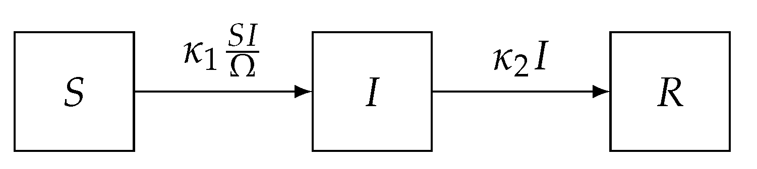For instance, when the size of the state space is finite, a solution to Equation (5) can be computed in principle via matrix exponentiation. Even when the state space is finite, it is usually very large, large enough so that exact solutions to the ME using matrix exponentiation is infeasible. For example, in the SIR model we fit to the Eyam plague data below, the size of the state space is 62,128. An exact solution to the ME via matrix exponentiation requires the computation of the power series of a 62,128 × 62,128 matrix, and this calculation would be required each time the likelihood needs to be evaluated at a particular parameter value.

To completely specify the stochastic systems under consideration, we must determine the form of the stochastic reaction rates $f_r$. Under the assumptions that the system is well-stirred and at constant temperature, these rates mirror the deterministic mass action rates and follow the so-called stochastic law of mass action of the form

$$f_r\left(X\right)={\kappa }_r\Omega \prod _{i=1}^d\frac{X_i!}{(X_i-{\eta }_{ir})!{\Omega }^{{\eta }_{ir}}}.$$

(6)

These are adjustments of the determinsitic rates that account for finite molecule numbers and the combinatorial number of ways to choose reactant molecules. A rigorous derivation of these rates was given by [6] and McQuarrie was one of the first to review the stochastic nature of chemically reacting systems [9]. Under the assumptions that the systems are well-mixed and thermally equilibrated, the reaction rates have the form in Equation (6) and the master equation with these rates describe a density dependent Markov process (DDMJP). DDMJPs evolve over continuous time and make jumps at discrete time points, which update the system’s state. Further, their transition probabilities depend on the state space only through the density $\frac{X}{\Omega }$, hence the name. We give two important results on the limiting properties of DDMJPs in the Appendix A developed by Tom Kurtz [10,11,12,13], which we make use of in Section 3 to prove results on the properties of the proposed estimation method. In the context of chemical systems, the master equation is often referred to as the chemical master equation (CME).

While exact solutions to the ME/CME are usually not available, several useful approximations have been developed which are more amenable to analysis. These often involve Taylor expanding the ME and truncating higher order terms. Consider writing the ME in terms of the step operator as follows

$${\displaystyle \frac{d}{dt}}P(X,t)=\sum _{r=1}^R(\prod _{i=1}^d{E}_i^{-S_{ir}}-1)f_r(X,t)P(X,t).$$

(7)

Here, $X_i$ is the number of molecules of species i and $E_i^{-S_{ir}}$ is the step operator defined by $E_i^{-S_{ir}}f(X_1,\cdots ,X_i,\cdots ,X_d)=f(X_1,\cdots ,X_i-S_{ir},\cdots ,X_d)$. Taylor expansion of the step operator and truncation of terms of order higher than 3 leads to a partial differential equation which gives an approximation to the ME. This partial differential equation is sometimes referred to as a Fokker–Planck equation, whose solution describes the probability distribution of a Langevin equation (CLE), or diffusion process. In general, a Fokker–Planck approximation will still not have analytic solutions, but simulating process trajectories from the CLE will be typically much more efficient than simulation from the exact process via Gillespie’s stochastic simulation algorithm (SSA). If we carry this out one step further and Taylor expand both the step operator and the rate functions $f_r$ about the ODE solution Equation (4), we arrive at yet another partial differential equation. The solution to this equation describes the probability distribution of the so-called linear noise approximation (LNA), see [14,15,16] for details on these expansions. The LNA has several nice properties that make it useful for computation, one of them being that the process variances and covariances can be computed by a matrix system of ODEs. The LNA process variance at time t, which we denote ${\Sigma }_t$, satisfies

$$\frac{d{\Sigma }_t}{dt}=A_t{\Sigma }_t+{\Sigma }_t{A}_t^{\top }+B_t{B}_t^{\top },$$

(8)

where $A_{ij}={\sum }_{r=1}^R{S}_{ir}\frac{\partial f_r\left(\varphi \right)}{\partial {\varphi }_j}$, $B=S\sqrt{diag\left(f\right(\varphi \left)\right)}$ and is subject to initial condition ${\Sigma }_0$. Note that $f\left(\varphi \right)$ is the vector $(f_1\left(\varphi \right),...,f_R\left(\varphi \right))$, and the explicit dependence on time t has been suppressed. Our goal was to use the ideas introduced in this section to propose a method for estimating the parameters ${\kappa }_r$ of a stochastic reaction network. We do this in the following section and prove results on properties of the proposed estimators.

3. Generalized Estimating Equations

Ideally, one would base the statistical estimation of parameters on the likelihood function. The likelihood principle has axiomatic foundations in statistical decision theory, and acceptance of the principle justifies using the likelihood function, as it then contains all the available information provided by the data [17,18,19]. As has been mentioned previously, unfortunately the likelihood function is generally intractable in the setting of stochastic reaction networks because of the intractability of the ME solution. A powerful tool to circumvent the intractability of the likelihood function uses a so-called particle filtering approach. This methodology relies on simulating trajectories, or particles, from the processes to obtain unbiased estimates of the likelihood function, and hence allows for exact Bayesian inference via particle marginal Metropolis–Hastings (PMMH) [20]. Even in the absence of some of the known issues associated with PMMH, such as particle degeneracy, merely the computational cost of implementing PMMH may be significant. This is due to the required sampling of particles, and the general difficulty related to tuning Markov chain Monte-Carlo (MCMC) proposal distributions in the absence of an analytic form for the likelihood function. We compare the proposed methodology to PMMH in our simulation study.

Likelihood-free methods have also been proposed to alleviate the outright need to compute the likelihood function. Approximate Bayesian computation (ABC) is a popular class of likelihood-free methods that require only the ability to simulate from the process [21]. While ABC methods are straightforward to implement, once appropriate summary statistics and distance measures have been selected, good choices for these are often not straightforward and will affect both the quality of the approximate posterior and the quality of the chain. We do not consider ABC methods further, since both PMMH and ABC require repeated sampling of the process, but PMMH can give exact posterior distributions instead of approximate posteriors. Further, PMMH does not require selection of statistics that are essentially guaranteed to not be sufficient by the Fisher–Pitman–Koopman–Darmois theorem.

Another likelihood-free method based on least squares estimates (LSE) for DDMJPs has been proposed in [22], and investigated further in [23]. Assume we have observed the process at timepoints $t_0,t_1,...,t_T$, leading to the data $\left\{X\left(t_0\right),X\left(t_1\right),...,X\left(t_T\right)\right\}$ where each $X\left(t_j\right)\in {\mathbb{R}}^d$. The least squares estimator is the solution to

$${\kappa }^{LSE}=\underset{\kappa }{\mathrm{argmin}}\sum _{j=1}^T{\left(x\left(t_j\right)-{\varphi }^{\kappa }\left(t_j\right)\right)}^{\top }\left(x\left(t_j\right)-{\varphi }^{\kappa }\left(t_j\right)\right),$$

where $x\left(t_j\right)=\frac{X\left(t_j\right)}{\Omega }$. The asymptotic properties of ${\kappa }^{LSE}$ have been investigated in [22]. Here, we propose a weighted estimator that accounts for the different variability in the process at different time points. Consider the solution to the following

$$\widehat{\kappa }=\underset{\kappa }{\mathrm{argmin}}\sum _{j=1}^T{\left(x\left(t_j\right)-{\varphi }^{\kappa }\left(t_j\right)\right)}^{\top }{V}_{t_j}^{-1}\left(x\left(t_j\right)-{\varphi }^{\kappa }\left(t_j\right)\right),$$

(9)

where $V_{t_j}$ is a symmetric positive definite matrix. Differentiating with respect to $\kappa$, setting to 0 and solving for $\kappa$ gives the proposed estimator $\widehat{\kappa }$, which is the solution to the estimating equation [24] $G_{\Omega }\left(\kappa \right)=0$, i.e.,

$$G_{\Omega }\left(\widehat{\kappa }\right)=\sum _{j=1}^T\frac{\partial {\varphi }^{\widehat{\kappa }}\left(t_j\right)}{\partial \kappa }{V}_{t_j}^{-1}\left(x\left(t_j\right)-{\varphi }^{\widehat{\kappa }}\left(t_j\right)\right)=0,$$

(10)

where $x\left(t_j\right)=\frac{X\left(t_j\right)}{\Omega }$ are the observed species concentrations and ${\varphi }^{\kappa }\left(t_j\right)$ is the ODE solution at time $t_j$. Generalized estimating equations (GEEs) have been used in the context of diffusion processes [25], and here we investigate them in the context of DDMJPs. For the proposed method, we estimate the process variance matrix $V_{t_j}$ by numerically solving the LNA variance formula in Equation (8). We prove two results on the limiting properties of the GEE estimator $\widehat{\kappa }$. The first result is on consistency, and the second a central limit theorem (CLT), using results of theorems provided in the Appendix A on the strong law of large numbers (SLLN) and the CLT for DDMJPs.

3.1. Consistency

Theorem 1

(Consistency). Let ${\partial }_r{\varphi }^{\kappa }$ denote the derivative of ${\varphi }^{\kappa }\in {\mathbb{R}}_{\ge 0}^d$ with respect to the rth coordinate of $\kappa \in {\mathbb{R}}_{+}^R$ and set $\partial {\varphi }^{\kappa }=[{\partial }_r{\varphi }_j^{\kappa }]\in {\mathbb{R}}^{R\times d}$. Assume that $\left|\right|\partial {\varphi }^{\kappa }\left|\right|<\infty$ and that the SLLN for the DDMJP holds. If

$$\forall {\kappa }_1,{\kappa }_2{\varphi }^{{\kappa }_1}\left(t_j\right)={\varphi }^{{\kappa }_2}\left(t_j\right)\mathrm{for}j=1\cdots ,T\mathrm{implies}{\kappa }_1={\kappa }_2,$$

(11)

and for some $ϵ>0$

$${\exists }_r\sum _j{\partial }_r{\varphi }^{\kappa }\left(t_j\right)V_{t_j}^{-1}\left({\varphi }^{\kappa }\left(t_j\right)-{\varphi }^{{\kappa }^0}\left(t_j\right)\right)\ne 0for\kappa \ne {\kappa }^0,\mid \kappa -{\kappa }^0\mid <ϵ,$$

(12)

then the GEE estimator is a strongly consistent estimate, that is $\widehat{\kappa }\to {\kappa }^0$ almost surely.

Proof. 

Assume that $x\left(t_j\right)$ are the observed concentrations from a density DDMJP and that ${\kappa }^0$ is the true parameter. Adding and subtracting ${\varphi }^{{\kappa }^0}\left(t_j\right)$ inside the parenthesis of Equation (10) we have

$$\begin{array}{cc}\hfill & {\displaystyle \sum _{j=1}^T}\frac{\partial {\varphi }^{\hat{\kappa }}\left(t_j\right)}{\partial \kappa }{V}_{t_j}^{-1}\left(x\left(t_j\right)-{\varphi }^{{\kappa }^0}\left(t_j\right)+{\varphi }^{{\kappa }^0}\left(t_j\right)-{\varphi }^{\widehat{\kappa }}\left(t_j\right)\right)=0\hfill \\ \hfill & {\displaystyle \sum _{j=1}^T}\frac{\partial {\varphi }^{\widehat{\kappa }}\left(t_j\right)}{\partial \kappa }{V}_{t_j}^{-1}\left(x\left(t_j\right)-{\varphi }^{{\kappa }^0}\left(t_j\right)\right)={\displaystyle \sum _{j=1}^T}\frac{\partial {\varphi }^{\widehat{\kappa }}\left(t_j\right)}{\partial \kappa }{V}_{t_j}^{-1}\left({\varphi }^{\widehat{\kappa }}\left(t_j\right)-{\varphi }^{{\kappa }^0}\left(t_j\right)\right).\hfill \end{array}$$

(13)

The SLLN for DDMJP given in Appendix A implies the left hand side (LHS) of Equation (13) converges to zero almost surely as $\Omega \to \infty$. Thus, we have in the large volume limit that

$$\sum _j\frac{\partial {\varphi }^{{\widehat{\kappa }}_{\infty }}\left(t_j\right)}{\partial \kappa }{V}_{t_j}^{-1}\left({\varphi }^{{\widehat{\kappa }}_{\infty }}\left(t_j\right)-{\varphi }^{{\kappa }^0}\left(t_j\right)\right)=0$$

(14)

almost surely, where ${\widehat{\kappa }}_{\infty }$ is the limiting solution to Equation (10). Under the assumptions in Equations (11) and (12), we thus have that ${\widehat{\kappa }}_{\infty }={\kappa }^0$ almost surely. □

3.2. Central Limit Theorem

Theorem 2

(Central limit theorem). Assume that all of the assumptions of Theorem 1 hold, that $V_{t_j}$ is invertible, and that the central limit theorem (CLT) hypotheses for DDMJP hold for the CLT in Appendix A. Then

$$\sqrt{\Omega }(\widehat{\kappa }-{\kappa }^0)\Rightarrow {\mathcal{N}}_R(0,{\Sigma }_{{\kappa }^0}),$$

(15)

where ${\mathcal{N}}_R$ denotes the R-variate normal distribution, ⇒ denotes convergence in distribution and ${\Sigma }_{{\kappa }^0}$ is given by

$$\begin{array}{ccc}\hfill {\Sigma }_{{\kappa }^0}& =& \sum _{j}Var\left(A_j{Z}_j\right)\hfill \\ & =& \sum _j{A}_{j}Var\left(Z_j\right)A_j^{\top }+\sum _{j<i}{A}_{j}Var(Z_j,Z_i)A_i^{\top }+\sum _{j<i}{A}_{i}Var(Z_i,Z_j)A_j^{\top }.\hfill \end{array}$$

In the above, $A_j={\mathbf{B}}_{{\kappa }^0}^{-1}{V}_{t_j}^{-1}\partial {\varphi }^{{\kappa }^0}$, ${\mathbf{B}}_{{\kappa }^0}={\sum }_{j=1}^T\partial {\varphi }^{{\kappa }^0}{V}_{t_j}^{-1}{[\partial {\varphi }^{{\kappa }^0}]}^{\top }$ and $Z_j$ is the limiting process ${lim}_{\Omega \to \infty }\sqrt{\Omega }\left(x\left(t_j\right)-c^{{\kappa }^0}\left(t_j\right)\right)$.

Proof. 

Consider the RHS of Equation (13), expanding this as a function of $\widehat{\kappa }$ about the point ${\kappa }^0$ we have

$$\begin{array}{cc}\hfill {\displaystyle \sum _{j=1}^T}\partial {\varphi }^{\hat{\kappa }}{V}_{t_j}^{-1}\left({\varphi }^{\widehat{\kappa }}\left(t_j\right)-{\varphi }^{{\kappa }^0}\left(t_j\right)\right)& ={\displaystyle \sum _{j=1}^T}\partial {\varphi }^{\widehat{\kappa }}{V}_{t_j}^{-1}\left({\varphi }^{{\kappa }^0}\left(t_j\right)-{\varphi }^{{\kappa }^0}\left(t_j\right)\right)+{\displaystyle \sum _{j=1}^T}\partial {\varphi }^{\widehat{\kappa }}{V}_{t_j}^{-1}{[\partial {\varphi }^{{\kappa }^0}]}^{\top }\left(\widehat{\kappa }-{\kappa }^0\right)\hfill \\ \hfill & +O(\mid \widehat{\kappa }-\kappa \mid )\left(\widehat{\kappa }-{\kappa }^0\right)\hfill \\ \hfill & ={\displaystyle \sum _{j=1}^T}[\partial {\varphi }^{\widehat{\kappa }}]V_{t_j}^{-1}{[\partial {\varphi }^{{\kappa }^0}]}^{\top }\left(\widehat{\kappa }-{\kappa }^0\right)+o_p\left(1\right)\left(\widehat{\kappa }-{\kappa }^0\right).\hfill \end{array}$$

(16)

The standard order bound $O(\mid \widehat{\kappa }-\kappa \mid )$ is directly from the Taylor’s expansion and the small o convergence in probability to 0 of this term, i.e., $o_p\left(1\right)$ follows from the previous result on the consistency of $\widehat{\kappa }$. Thus, the second term on the RHS of Equation (16) converges to 0 in probability and may be neglected. Defining ${\mathbf{B}}_{\widehat{\kappa }}$ as ${\mathbf{B}}_{\widehat{\kappa }}={\sum }_{j=1}^T\partial {\varphi }^{\widehat{\kappa }}{V}_{t_j}^{-1}{[\partial {\varphi }^{{\kappa }^0}]}^{\top }$ and considering the remaining terms we have that

$${\mathbf{B}}_{\widehat{\kappa }}\left(\widehat{\kappa }-{\kappa }^0\right)=\sum _{j=1}^T\partial {\varphi }^{\widehat{\kappa }}{V}_{t_j}^{-1}\left(x\left(t_j\right)-{\varphi }^{{\kappa }^0}\left(t_j\right)\right).$$

Inverting by ${\mathbf{B}}_{\widehat{\kappa }}$ and scaling by $\sqrt{\Omega }$ gives

$$\sqrt{\Omega }(\widehat{\kappa }-{\kappa }^0)=\sum _{j=1}^T{\mathbf{B}}_{\widehat{\kappa }}^{-1}\partial {\varphi }^{\widehat{\kappa }}{V}_{t_j}^{-1}\sqrt{\Omega }\left(x\left(t_j\right)-{\varphi }^{{\kappa }^0}\left(t_j\right)\right).$$

Since $\widehat{\kappa }$ converges to ${\kappa }^0$ almost surely, it also converges in probability, which implies that ${\mathbf{B}}_{\widehat{\kappa }}^{-1}\partial {\varphi }^{\widehat{\kappa }}\to {\mathbf{B}}_{{\kappa }^0}^{-1}\partial {\varphi }^{{\kappa }^0}$ in probability. Therefore,

$$\sqrt{\Omega }(\widehat{\kappa }-{\kappa }^0)\Rightarrow \sum _{j=1}^T{\mathbf{B}}_{{\kappa }^0}^{-1}\partial {\varphi }^{{\kappa }^0}{V}_{t_j}^{-1}\sqrt{\Omega }\left(x\left(t_j\right)-{\varphi }^{{\kappa }^0}\left(t_j\right)\right).$$

From the CLT theorem for DDMJPs given in Appendix A, we have that $\sqrt{\Omega }(x(t_j)-{\varphi }^{{\kappa }^0}(t_j))$ converges in distribution to the d-variate normal, with mean 0 and variance $Var\left(Z_j\right)$. Therefore, we have that $\sqrt{\Omega }(\widehat{\kappa }-{\kappa }^0)\Rightarrow MVN(0,{\Sigma }_{{\kappa }^0})$, as required. □

Note that in the above theorems, we have assumed that the data come from a single trajectory of the DDMJP; however, the results may be extended to data collected from independent trajectories of the jump process. This will be the case when the data collection process is destructive, for example those requiring crushing of cells. If we have data from multiple trajectories that are independent, then the Cov $(Z_j,Z_i)=0$ for $i\ne j$, and under the remaining conditions the results still hold but then with ${\Sigma }_{{\kappa }^0}={\sum }_j{A}_{j}Var\left(Z_j\right)A_j^{\top }$.

4. Simulation

For our simulation study we consider the classical Lotka–Volterra model with two species, rabbit (Ra) and fox (F), and the corresponding reaction network given below by

$$\begin{array}{cc}\hfill Ra& \stackrel{{\kappa }_1}{\to }2Ra\hfill \\ \hfill Ra+F& \stackrel{{\kappa }_2}{\to }2F\hfill \\ \hfill F& \stackrel{{\kappa }_3}{\to }⌀\hfill \end{array}$$

Accordingly, the stoichiometric matrix $S={\eta }^{\prime }-\eta$ is

$$\begin{array}{cccc}& R_1& R_2& R_3\\ Ra& 1& -1& 0\\ F& 0& 1& -1\end{array}$$

(17)

with the macroscopic mass action rates

$$g\left(x\right)={({\kappa }_1{x}_1,{\kappa }_2{x}_1{x}_2,{\kappa }_3{x}_2)}^T,$$

and where $x_1$ and $x_2$ are concentration of rabbits and foxes, respectively. The macroscopic rate equations for the LV system have the form

$$\begin{array}{ccc}\hfill \frac{d}{dt}{\varphi }_1& =& {\kappa }_1{\varphi }_1-{\kappa }_2{\varphi }_1{\varphi }_2\hfill \\ \hfill \frac{d}{dt}{\varphi }_2& =& {\kappa }_2{\varphi }_1{\varphi }_2-{\kappa }_3{\varphi }_2.\hfill \end{array}$$

(18)

For the simulation study, we generate trajectories from the stochastic LV process using Gillespie’s SSA, and we collect the observed data at 10 evenly spaced time points in the interval (0.1,1) under three different volume sizes $\Omega$ = 1, 10 and 100. We set the parameter values to ${\kappa }_1=1,{\kappa }_2=0.2,{\kappa }_3=0.5$, and the initial rabbit and fox copy numbers are set so that the initial concentrations are $x_1=10$ and $x_2=10$ under each of the different volume scenarios. For the particle filtering method, which we label as (PMMH) in the tables, we used 100 particles generated from Gillespie’s SSA and a standard deviation of 10 for the measurement error to construct the likelihood. We implement two numerical procedures for the proposed GEE method. The first uses a single iteration of the GEE solution, with the process variance $V_{t_j}$ for this single iteration computed using the LNA variance formula evaluated using the LSE solution. We denote this as ${\mathrm{GEE}}_1$. The second implementation updates the process variance $V_{t_j}$ at the each iteration by using the previous iterations GEE estimate until convergence. We denote this as GEE. We initialize each of these numerical procedures at the LSE for the starting point. We report the average of the parameter estimates over the 1000 iterations for each method. For the proposed method we report the coverage probabilities of 95% confidence intervals constructed using the CLT result proven in the previous section, which are in parenthesis in the tables below.

The results in

Table 1. Lotka–Volterra (LV) model estimates for GEE, ${\mathrm{GEE}}_1$, LSE and particle marginal Metropolis–Hastings (PMMH) at $\Omega =1$ and $\Omega =10$.

	$\mathbf{\Omega }=\mathbf{1}$				$\mathbf{\Omega }=\mathbf{10}$
Method	GEE	${\mathbf{GEE}}_{\mathbf{1}}$	LSE	PMMH	GEE	${\mathbf{GEE}}_{\mathbf{1}}$	LSE	PMMH
Hrs	0.01	0.02	0.01	0.84	0.07	0.05	0.02	1.25
${\kappa }_1$ = 1	1.2 (0.94)	1.3 (0.96)	1.82	0.92	1 (0.94)	1.1(0.96)	1.02	1.02
${\kappa }_2$ = 0.2	0.2 (0.95)	0.2 (0.97)	0.27	0.32	0.2 (0.94)	0.21(0.97)	0.2	0.2
${\kappa }_3$ = 0.5	0.6 (0.95)	0.6 (0.98)	0.96	0.68	0.5 (0.95)	0.52 (0.98)	0.5	0.5

and

Table 2. LV model estimates for GEE, ${\mathrm{GEE}}_1$, LSE and PMMH at $\Omega =100$.

	$\mathbf{\Omega }=\mathbf{100}$
Method	GEE	${\mathbf{GEE}}_{\mathbf{1}}$	LSE	PMMH
Hrs	0.08	0.05	0.02	2.15
${\kappa }_1$ = 1	1.01 (0.95)	1.02 (0.95)	0.99	1
${\kappa }_2$ = 0.2	0.2 (0.98)	0.20 (0.98)	0.2	0.3
${\kappa }_3$ = 0.5	0.51 (0.94)	0.51 (0.95)	0.5	0.55

indicate that the proposed methodology works reasonably well for a range of volumes in the LV system. For instance, we see that already at a volume of $\Omega =1$, the GEE estimates are close to the true values and that the empirical coverage probabilities are close to the nominal level. This implies that, in this example, the asymptotic normality of the estimates is generally a good approximation even at this small volume. Further, the proposed GEE method appears to be less biased than the LSE and PMMH at this volume size. Further, as the volume increases, the estimates for GEE and LSE methods tend toward the truth, while for $\Omega =100$ the PMMH estimates for ${\kappa }_2$ still maintain some bias.

In

Table 3. Comparing the different methods at $\Omega =1$.

Methods	GEE		${\mathbf{GEE}}_{\mathbf{1}}$		LSE		PMMH
$\kappa$	Var	${\mathrm{Bias}}^2$	Var	${\mathrm{Bias}}^2$	Var	${\mathrm{Bias}}^2$	Var	${\mathrm{Bias}}^2$
${\kappa }_1$	1.38	1.42	1.86	1.94	8.61	9.28	0.46	0.45
${\kappa }_2$	0.01	0.01	0.01	0.02	0.05	0.05	0.02	0.03
${\kappa }_3$	0.35	0.36	0.74	0.76	2.88	3.09	0.13	0.16

,

Table 4. Comparing the different methods at $\Omega =10$.

Methods	GEE		${\mathbf{GEE}}_{\mathbf{1}}$		LSE		PMMH
$\kappa$	Var	${\mathrm{Bias}}^2$	Var	${\mathrm{Bias}}^2$	Var	${\mathrm{Bias}}^2$	Var	${\mathrm{Bias}}^2$
${\kappa }_1$	0.19	0.19	0.23	0.21	0.16	0.16	0.06	0.11
${\kappa }_2$	0.001	0.001	0.001	0.002	0.001	0.001	0.09	0.22
${\kappa }_3$	0.03	0.03	0.04	0.03	0.02	0.02	0.03	0.06

and

Table 5. Comparing the different methods at $\Omega =100$.

Methods	GEE		${\mathbf{GEE}}_1$		LSE		PMMH
$\kappa$	Var	${\mathrm{Bias}}^2$	Var	${\mathrm{Bias}}^2$	Var	${\mathrm{Bias}}^2$	Var	${\mathrm{Bias}}^2$
${\kappa }_1$	0.02	0.02	0.02	0.02	0.01	0.01	0.35	0.35
${\kappa }_2$	0.0001	0.0001	0.0001	0.0001	0.0001	0.0001	0.08	0.11
${\kappa }_3$	0.002	0.002	0.003	0.003	0.002	0.002	0.34	0.39

, we compare the variance and squared-bias for each parameter using the different methods on the LV model. At small volume $\Omega =1$, the PMMH has the smallest variance and bias, followed by the GEE and then LSE. Although the PMMH method performs well for the LV model in the smallest volume $\Omega =1$ case, this comes at the cost of significant increase in computational time compared to both the GEE and LSE, which are approximately 20 and 60 times faster, respectively. At larger volumes this time difference becomes even more pronounced due to having to simulate particles via the Gillespie SSA for the PMMH method. Further, at least in the LV example, as the volume increases above 1, both the estimates and run time are better for the GEE method compared to PMMH. Hence, one may consider using the GEE at moderate to high volumes ($\Omega \ge 10$), and PMMH at very low volumes, provided the computation time is feasible.

5. Real Data Application: Eyam Plague of 1665–1666

We now apply our methodology to real data from a historical plague outbreak at Eyam, England. The Eyam plague of 1666 in England started in 1665 when a flea-infested bundle of cloth arrived from London for a local tailor. The tailor’s assistant, George Vicars, was the first fatality, and he died within a week of the arrival. As more people began dying via disease transmission throughout the village, Reverend William Mompesson and Minister Thomas Stanley introduced precautions to slow the spread of the illness from May 1666. These included families burying their own dead and quarantining the entire village. The worst month of the outbreak was August 1666, during which there were five to six deaths per day. We used the proposed methodology to estimate the epidemiological parameters of a stochastic SIR compartmental model for this outbreak. The plague lasted for over 14 months nearly wiping out the entire village. Abraham Morten was the last victim of the plague, dying on 1 November 1666. We modeled this outbreak with an SIR model, where S is susceptible, I is infectious and R is removed. The initial number of people who lived in the village at the time of the outbreak and how many people died is subject to debate and has been revised several times Whittles and Didelot [26], but we use numbers based on the account of historian William Wood about the village’s demography [27]. Wood wrote about this outbreak a century after the event. According to Wood, there were about 350 people in the village, with the plague killing $75\%$ of villagers. In this example of a fixed closed population, a natural quantity for the system volume is $\Omega =350$, the total population.

The SIR diagram in Figure 1. depicts how individuals can transition between the compartments. For instance, a susceptible may transition to the infectious compartment by interacting with an infectious contact. The rate describing movement from the S compartment to the I compartment is proportional to the rate constant ${\kappa }_1$ times the number of possible pair-wise interactions between infected and susceptible individuals, $SI$. Additionally, an infected individual transitions to the R compartment at rate ${\kappa }_2$. The macroscopic rate equations for the SIR model are

$$\begin{array}{ccc}\hfill \frac{dS}{dt}& =& -{\kappa }_{1}SI,\hfill \\ \hfill \frac{dI}{dt}& =& {\kappa }_{1}SI-{\kappa }_{2}I.\hfill \end{array}$$

While transmission via flea bites is almost certainly how the outbreak initially began, it became clear during the latter months that human-to-human transmission was a driving force. It was reported that the infection could eventually be spread from the cough of an infectious person. This route of infectious spread is sometimes referred to as plague pneumonia, and the SIR system offers a simple model of the human-to-human transmission. We also look at a model that includes a vector, in this case representing rats, as a possible mode of transmission through flea bites. We assume a constant infectious pressure from the vector compartment V, and we denote this model as SIRV. A graphical depiction of this model is dislplayed in the Figure 2 below.

The corresponding rate equations are given below.

$$\begin{array}{cc}\hfill \frac{dS}{dt}=& -{\kappa }_{1}SI-{\kappa }_{3}S,\hfill \\ \hfill \frac{dI}{dt}=& {\kappa }_{1}SI+{\kappa }_{3}S-{\kappa }_{2}I.\hfill \end{array}$$

Table 6. Data of susceptible and infectious at 8 different time points for the Eyam plague outbreak.

Time (Months)	0	1	1.5	2	2.5	3	3.5	4
Susceptible	254	235	201	153	121	110	97	83
Infectives	7	14	22	29	20	8	8	0

contains the number of susceptible and infected individuals at 8 time points over a 4 month period from 18 May 1666 to 19 September 1666 [27]. We fit both the SIR and SIRV models to these data using the GEE and LSE methods and report the results in

Table 7. Parameter estimates for the SIR and SIRV models fit to the Eyam plague data.

	SIR Model
Method	GEE	${\mathrm{GEE}}_1$	LSE
Time (s)	16.31	4.28	0.58
${\kappa }_1$	4.69 (4.59, 4.78)	4.71 (4.58, 4.83)	4.68 (4.42, 4.93)
${\kappa }_2$	2.75 (2.64, 2.86)	2.77 (2.37, 3.17)	2.89 (2.51, 3.26)
	SIRV Model
Time (s)	16.02	6.65	0.78
${\kappa }_1$	4.75	4.74	4.52
${\kappa }_2$	2.94	2.94	2.78
${\kappa }_3$	0	0	0

.

For the SIRV model, the estimated vector transmission parameter ${\kappa }_3$ is zero for all the methods, which suggests that this mode of transmission may not have played as significant a role in the disease transmission as has been originally suggested, at least after the infection has been initiated. Thus, the results from these analyses indicate it is likely most people were infected through some form of human-to-human transmission at the Eyam outbreak, either through plague pneumonia or ectoparasites, like lice. Hence, the SIRV model reduces to the standard SIR model in this case. The 95% confidence intervals for the SIR model parameters in parenthesis indicate the GEE method has increased precision compared to the LSE as the interval widths are more than twice as large for the LSE. The ${\mathrm{GEE}}_1$ method also has interval width around two times smaller than the LSE’s interval width for ${\kappa }_1$, and has similar widths for ${\kappa }_2$. These estimated parameters give basic reproductive rate estimates of ${\mathcal{R}}_0^{\mathrm{GEE}}=1.71$, ${\mathcal{R}}_0^{{\mathrm{GEE}}_1}=1.70$ and ${\mathcal{R}}_0^{\mathrm{LSE}}=1.62$. We plot the corresponding macroscopic rate equations solution for the SIR model with the estimated parameter values from the two GEE methods.

The ODE curves in Figure 3 give an estimated final outbreak size of approximately $70\%$ for both methods, which is similar to the observed final outbreak size.

6. Discussion

In this paper we have proposed a new way to estimate the parameters of stochastic reaction networks. We used ideas related to generalized estimating equations to estimate these parameters using the covariance matrix computed from the LNA’s approximating variance. We have discussed why stochastic models are a better way to model reaction networks compared to the classical deterministic models. While the CME gives us an exact representation for reaction networks, the computational cost of computing the CME quickly becomes prohibitive, and thus approximate methods can help tackle this issue. The ability to reverse engineer reaction networks from experimental data is critical for understanding and predicting a variety of biological systems’ behavior. Thus, we have proposed methodology for estimating parameters when we have observed data from stochastic reaction networks, and we have developed the corresponding limiting results so that researchers may perform better inferences about their systems.

References

1. Albert, R. Network inference, analysis, and modeling in systems biology. Plant Cell 2007, 19, 3327–3338. [Google Scholar] [CrossRef] [Green Version]
2. Bonneau, R. Learning biological networks: From modules to dynamics. Nat. Chem. Biol. 2008, 4, 658. [Google Scholar] [CrossRef]
3. Gardner, T.S.; Faith, J.J. Reverse-engineering transcription control networks. Phys. Life Rev. 2005, 2, 65–88. [Google Scholar] [CrossRef]
4. Wilkinson, D.J. Stochastic Modelling for Systems Biology; Chapman and Hall/CRC: Boca Raton, FL, USA, 2006. [Google Scholar]
5. Gillespie, D.T. Exact stochastic simulation of coupled chemical reactions. J. Phys. Chem. 1977, 81, 2340–2361. [Google Scholar] [CrossRef]
6. Gillespie, D.T. A rigorous derivation of the chemical master equation. Phys. A Stat. Mech. Its Appl. 1992, 188, 404–425. [Google Scholar] [CrossRef]
7. Guldberg, C.; Waage, P. Studies concerning affinity CM Forh.: Vidensk. Selsk. Christ. 1886, 35. [Google Scholar] [CrossRef]
8. Klipp, E.; Herwig, R.; Kowald, A.; Wierling, C.; Lehrach, H. Systems Biology in Practice: Concepts, Implementation and Application; John Wiley & Sons: New York, NY, USA, 2008. [Google Scholar]
9. McQuarrie, D.A. Stochastic approach to chemical kinetics. J. Appl. Probab. 1967, 4, 413–478. [Google Scholar] [CrossRef]
10. Kurtz, T.G. Solutions of ordinary differential equations as limits of pure jump Markov processes. J. Appl. Probab. 1970, 7, 49–58. [Google Scholar] [CrossRef]
11. Kurtz, T.G. The relationship between stochastic and deterministic models for chemical reactions. J. Chem. Phys. 1972, 57, 2976–2978. [Google Scholar] [CrossRef]
12. Kurtz, T.G. Limit theorems and diffusion approximations for density dependent Markov chains. In Stochastic Systems: Modeling, Identification and Optimization, I; Springer: Berlin, Germany, 1976; pp. 67–78. [Google Scholar]
13. Kurtz, T.G. Strong approximation theorems for density dependent Markov chains. Stoch. Process. Their Appl. 1978, 6, 223–240. [Google Scholar] [CrossRef] [Green Version]
14. Van Kampen, N.G. Stochastic Processes in Physics and Chemistry; Elsevier: Amsterdam, The Netherlands, 1992; Volume 1. [Google Scholar]
15. Komorowski, M.; Finkenstädt, B.; Harper, C.V.; Rand, D.A. Bayesian inference of biochemical kinetic parameters using the linear noise approximation. BMC Bioinform. 2009, 10, 343. [Google Scholar] [CrossRef] [Green Version]
16. Komorowski, M.; Costa, M.J.; Rand, D.A.; Stumpf, M.P. Sensitivity, robustness, and identifiability in stochastic chemical kinetics models. Proc. Natl. Acad. Sci. USA 2011, 108, 8645–8650. [Google Scholar] [CrossRef] [PubMed] [Green Version]
17. Fisher, R.A.; Russell, E.J. On the mathematical foundations of theoretical statistics. Philos. Trans. R. Soc. Lond. Ser. A Contain. Pap. Math. Phys. Character 1922, 222, 309–368. [Google Scholar] [CrossRef] [Green Version]
18. Birnbaum, A. On the Foundations of Statistical Inference. J. Am. Stat. Assoc. 1962, 57, 269–306. [Google Scholar] [CrossRef]
19. Berger, J.O.; Wolpert, R.L. Chapter 3: The Likelihood Principle and Generalizations. In The Likelihood Principle; Lecture Notes–Monograph Series; Institute of Mathematical Statistics: Hayward, CA, USA, 1988; Volume 6, pp. 19–64. [Google Scholar] [CrossRef]
20. Golightly, A.; Wilkinson, D.J. Bayesian parameter inference for stochastic biochemical network models using particle Markov chain Monte Carlo. Interface Focus 2011, 1, 807–820. [Google Scholar] [CrossRef] [PubMed] [Green Version]
21. Marjoram, P.; Molitor, J.; Plagnol, V.; Tavaré, S. Markov chain Monte Carlo without likelihoods. Proc. Natl. Acad. Sci. USA 2003, 100, 15324–15328. [Google Scholar] [CrossRef] [Green Version]
22. Rempala, G.A. Least squares estimation in stochastic biochemical networks. Bull. Math. Biol. 2012, 74, 1938–1955. [Google Scholar] [CrossRef]
23. Linder, D.F.; Rempała, G.A. Bootstrapping least-squares estimates in biochemical reaction networks. J. Biol. Dyn. 2015, 9, 125–146. [Google Scholar] [CrossRef] [PubMed] [Green Version]
24. Liang, K.Y.; Zeger, S.L. Longitudinal data analysis using generalized linear models. Biometrika 1986, 73, 13–22. [Google Scholar] [CrossRef]
25. Bibby, B.M.; Sørensen, M. Martingale estimation functions for discretely observed diffusion processes. Bernoulli 1995, 1, 17–39. [Google Scholar] [CrossRef]
26. Whittles, L.K.; Didelot, X. Epidemiological analysis of the Eyam plague outbreak of 1665–1666. Proc. R. Soc. B Biol. Sci. 2016, 283, 20160618. [Google Scholar] [CrossRef] [PubMed] [Green Version]
27. Raggett, G.F. A Stochastic Model Of The Eyam Plague. J. Appl. Stat. 1982, 9, 212–225. [Google Scholar] [CrossRef]
Figure 1. Susceptible, infectious recovered (SIR) compartmental model for the Eyam plague.
Mathematics 09 00391 g001
Figure 2. Susceptible, infectious recovered, vector(rats) (SIRV) compartmental model for the Eyam plague.
Mathematics 09 00391 g002
Figure 3. Plots of the SIR model ordinary differential equation (ODE) curves using the estimated parameter values from the Eyam plague data. (a) GEE SIR model for Eyam. (b) GEE 1 SIR model for Eyam data.
Mathematics 09 00391 g003