A Complex Model via Phase-Type Distributions to Study Random Telegraph Noise in Resistive Memories

Abstract

A new stochastic process was developed by considering the internal performance of macro-states in which the sojourn time in each one is phase-type distributed depending on time. The stationary distribution was calculated through matrix-algorithmic methods and multiple interesting measures were worked out. The number of visits distribution to a determine macro-state were analyzed from the respective differential equations and the Laplace transform. The mean number of visits to a macro-state between any two times was given. The results were implemented computationally and were successfully applied to study random telegraph noise (RTN) in resistive memories. RTN is an important concern in resistive random access memory (RRAM) operation. On one hand, it could limit some of the technological applications of these devices; on the other hand, RTN can be used for the physical characterization. Therefore, an in-depth statistical analysis to model the behavior of these devices is of essential importance.

1. Introduction

In several fields, such as computing and electronics engineering, it is of great interest to analyze complex devices with several macro-states that evolve by time. It is usual to consider Markov processes for this analysis, but in multiple occasions, the spent times in each macro-state are not exponentially distributed. In this context, a new approach is to consider that the spent time in each macro-state is phase-type (PH) distributed. In this case, it is assumed that each macro-state is composed of internal performance states that have a Markovian behavior. One interesting aspect is that the modeling of the stochastic process can only occur when the macro-state process can be observed. For this new process, the Markovianity is lost.

A phase-type distribution is defined as the distribution of the absorption time in an absorbing Markov chain. These probability distributions constitute a class of distributions on the positive real axis, which seems to strike a balance between generality and tractability, thanks to its good properties. This class of distributions was introduced by Neuts [1,2] and allows the modeling of complex problems in an algorithmic and computational way. It has been widely applied in fields such as engineering to model complex systems [3,4,5], queueing theory [6], risk theory [7] and electronics engineering [8].

The good properties of PH distributions due to their appealing probabilistic arguments constitute their main feature of being mathematically tractable. Several well-known probability distributions, e.g., exponential, Erlang, Erlang generalized, hyper-geometric, and Coxian distributions, among others, are particular cases of PH. One of the most important PH properties is that whatever nonnegative probability distribution can be approximated as much as desired through a PH, accounting for the fact that the PH class is dense in the set of probability distributions on the nonnegative half-line [9]. It allows the consideration of general distributions through PH approximations. Exact solutions to many complex problems in stochastic modeling can be obtained either explicitly or numerically by using matrix-analytic methods. The main features of PH distributions are described in depth in [10].

A macro-state stochastic process is built here to model the behavior of different random telegraph noise (RTN) signals. Given that the behavior of the different macro-states (levels) is not exponentially distributed, we assume each level to be composed of multiple internal phases that can be related with other levels. We show that if the internal process, by considering internal states inside the macro-states, has a Markovian behavior, the process between levels is not. For the latter, the sojourn time in each level is phase-type distributed depending on the initial time. This fact is of great interest and gives us more information about the device’s internal process.

Advanced statistical techniques are key tools to model complex physical and engineering problems in many different areas of expertise. In this context, a new statistical methodology is presented; we will concentrate in the study of resistive memories [11,12], also known as resistive random access memories (RRAMs), a subgroup of a wide class of electron devices named memristors [13]. They constitute a promising technology with great potential in several applications in the integrated circuit realm.

Circuit design is a tough task because of the high number of electronic components included in integrated circuits, therefore, electronic design automation (EDA) tools are essential. These software tools need compact models that represent the physics of the devices in order to fulfil their role in aiding circuit design. Although there are many works in compact modeling in the RRAM literature [14,15], there is a lot to be done, in particular in certain areas related to variability and noise. Variability is essential in modeling due to the RRAM operation’s inherent stochasticity, since the physics is linked to random physical mechanisms [16,17]. Another issue of great importance in these devices is noise. Among the different types of noise, random telegraph noise is of great concern [18]. The disturbances produced by one or several traps (physical active defects within the dielectric) inside the conductive filament or close to it alter charge transport mechanisms and consequently, current fluctuations can occur (Figure 1) that lead to RTN [14,15,19,20]. This noise can affect the correct device operation in applications linked to memory-cell arrays and neuromorphic hardware [14,16,21], posing important hurdles to the use of this technology in highly scaled integrated circuits. Nevertheless, RTN fluctuations can also be beneficial, for instance, when used as entropy sources in random number generators, an employment of most interest in cryptography [22,23].

The application in this issue is addressed in the current work, in particular with the statistical description of RTN signals in RRAMs. This study, in addition to physically characterizing the devices, can be used for compact modeling and, therefore, as explained above, for developing the software tools needed for circuit design. Accounting for the aforementioned intrinsic stochasticity of these devices, the choice of a correct statistical strategy to attack this problem is essential in the analysis. In this respect, we use the PH distributions, which have already been employed to depict some facets of RRAM variability [24]; nonetheless, as far as we know, they have not been used in RTN analysis.

In our study, we deal with devices whose structure is based on the Ni/HfO₂/Si stack. The fabrication details, as well as their electric characterization, are given in [25]. RTN measurements were recorded in the time domain by means of an HP-4155B semiconductor parameter analyzer (Figure 1). The current fluctuation between levels (see the marked levels in red in Figure 1), ΔI, and the spent time in each of the levels are key parameters to analyze. The associated time with the current low level is known as emission time (τ_e), which is linked to the time the active defect keeps a “captured” electron trapped until it releases it (through this time, it is said that the defect is occupied). On the other hand, the capture time (τ_c) represents the time taken to capture an electron by an empty defect.

The manuscript is organized as follows: in Section 2, the proposed statistical procedure is described; in Section 3, we deepen on the measures associated; and in Section 4, the number of visits to a determined macro-state is presented. The parameter estimation is unfolded in Section 5, and the application of the methodology developed here in Section 6. Finally, conclusions related to the main contributions of this work are presented in Section 7.

2. Statistical Methodology

Different RTN signals have been employed here, such as the ones shown in Figure 1. We have determined the number of current levels in order to be able to calculate the emission and capture times for a certain time interval. The current thresholds (red lines in Figure 1) were chosen to allow the extraction algorithm to calculate the time intervals corresponding to the levels defined previously.

In order to explain these issues, a new model is first built in transient and stationary regimes.

2.1. The Model

We assume a stochastic process {X(t); t ≥ 0} with macro-state space $E=\left\{1,2,\dots ,r\right\}$. Each macro-state k, level k, is composed of n_k internal phases or states denoted as $i_h^k$ for h = 1,…,n_k. We assume that the device internal performance is governed by a Markov process, {J(t); t ≥ 0}, with state space $E=\left\{i_1^1,\dots ,i_{n_1}^1,i_1^2,\dots ,i_{n_2}^2,\dots ,i_1^r,\dots ,i_{n_r}^r\right\}$, and with an initial distribution θ, and the following generator matrix expressed by blocks:

$$Q=\left(\begin{array}{ccccc}{Q}_{11}& \cdots & Q_{1k}& \cdots & Q_{1r}\\ & \ddots & & & \\ ⋮& & Q_{kk}& & ⋮\\ & & & \ddots & \\ Q_{r1}& \cdots & Q_{rk}& \cdots & Q_{rr}\end{array}\right)$$

where the matrix block Q_ij contains the transition intensities between the states of the macro-states from i to j.

Throughout this work, we will denote $Q_k$ as the matrix with zeros except the column matrix block k of Q, and $Q_{-k}$ as the matrix Q with zeros in the k-th block column. These matrices give the transition intensities of macro-state k and of any macro-state different to k, respectively.

Thus:

$$Q_k=\left(\begin{array}{ccccccc}0& \dots & 0& Q_{1k}& 0& \dots & 0\\ ⋮& \dots & ⋮& ⋮& ⋮& \dots & ⋮\\ 0& \dots & 0& Q_{rk}& 0& \dots & 0\end{array}\right)$$

$$Q_{-k}=\left(\begin{array}{ccccccc}{Q}_{11}^{}& \dots & Q_{1,k-1}^{}& 0& Q_{1,k+1}^{}& \dots & Q_{1r}^{}\\ ⋮& \dots & ⋮& ⋮& ⋮& \dots & ⋮\\ Q_{r1}^{}& \dots & Q_{r,k-1}^{}& 0& Q_{r,k+1}^{}& \dots & Q_{rr}^{}\end{array}\right)$$

It can be seen that the following equality holds: $Q=Q_k+Q_{-k}.$

Given the Q-matrix of the Markov process, the transition probability matrix for the process {J(t); t ≥ 0} is given by P(t) = exp{Qt}. From this and from the initial distribution θ, the transient distribution at time t is given by (P{X(t) = $i_1^1$}, P{X(t) = $i_2^1$},…, P{X(t) = $i_{n_r}^r$}) = a(t) = θ⋅P(t). The order of this vector is $1\mathrm{x}{\displaystyle {\sum }_{i=1}^r{n}_i}$.

The transition probabilities for the process {X(t); t ≥ 0} can be obtained from the transition probabilities of the Markov process {J(t); t ≥ 0}. If it is denoted as H(⋅,⋅) where the transition between macro-states i→j is given by:

$$\begin{array}{ll}{h}_{ij}\left(s,t\right)=P\left\{X\left(t\right)=j|X\left(s\right)=i\right\}& =\frac{{\displaystyle \sum _{h\in j}{\displaystyle \sum _{k\in i}P\left\{J\left(t\right)=h|J\left(s\right)=k\right\}P\left\{J\left(s\right)=k\right\}}}}{{\displaystyle \sum _{k\in i}P\left\{J\left(s\right)=k\right\}}}\\ & =\frac{{\displaystyle \sum _{k\in i}\left[a_k\left(s\right){\displaystyle \sum _{h\in j}{p}_{kh}\left(t-s\right)}\right]}}{{\displaystyle \sum _{k\in i}{a}_k\left(s\right)}}.\end{array}$$

This transition probability can be expressed in a matrix-algorithmic form as follows. Denoting by A_k a matrix of zeros with order ${\displaystyle {\sum }_{i=1}^r{n}_i}\mathrm{x}{\displaystyle {\sum }_{i=1}^r{n}_i}$ except the block corresponding to the macro-state k, which is the identity matrix, then:

$$h_{ij}\left(s,t\right)=P\left\{X\left(t\right)=j|X\left(s\right)=i\right\}=\frac{a\left(s\right)A_{i}P\left(t-s\right)A_j\cdot e}{a\left(s\right)A_i\cdot e}$$

where a(t)A_ie is the probability of being in the macro-state i at time t, with e being a column vector of ones with an appropriate order. A similar reasoning can be done with the embedded jumping probability.

Note that the matrix H is a stochastic matrix, and therefore it is a transition matrix of a Markov process. However, an important remark is that the Markov process related to the matrix H does not correspond to the process defined in this section. In fact, this process is non-homogeneous and not Markovian.

2.2. Stationary Distribution

The stationary distribution for the process {X(t); t ≥ 0} can be calculated by blocks from the stationary distribution for the process {J(t); t ≥ 0}. It is well known that this distribution verifies the balance equations $\pi Q=0$ and the normalization equation $\pi e=1$. We denote ${\pi }_k$ as the block of $\pi$ corresponding to the macro-state k. It is denoted as ${\pi }_k$e (k = 1,...,r) to the stationary distribution for the macro-state k of the process {X(t); t ≥ 0}.

The stationary distribution has been worked out by blocks in order to reduce the computational cost, according to the macro-states, and applying matrix-analytic methods.

As stated above, the stationary distribution verifies the following system:

$$\begin{array}{l}{\pi }_1{Q}_{11}+{\pi }_2{Q}_{21}+{\pi }_3{Q}_{31}+\cdots +{\pi }_r{Q}_{r1}=0\\ {\pi }_1{Q}_{12}+{\pi }_2{Q}_{22}+{\pi }_3{Q}_{32}+\cdots +{\pi }_r{Q}_{r2}=0\\ {\pi }_1{Q}_{13}+{\pi }_2{Q}_{23}+{\pi }_3{Q}_{33}+\cdots +{\pi }_r{Q}_{r3}=0\\ \cdots \\ {\pi }_1{Q}_{1r}+{\pi }_2{Q}_{2r}+{\pi }_3{Q}_{3r}+\cdots +{\pi }_r{Q}_{rr}=0\\ \pi \cdot e=1.\end{array}$$

It has been solved by using matrix-analytics methods, and the solution is given by

$${\pi }_j=-{\displaystyle \sum _{i=1}^{j-1}{\pi }_i{R}_{ij}^{r-j+1}};j=2,\dots ,r$$

where $R_{ij}^1=Q_{ij}{Q}_{jj}^{-1}$ for any i, j = 1,…, r with i ≠ j

$$R_{ij}^{r-j+1}=\left(R_{ij}^1+H_{ij}^{r-j+1}\right){\left(I+H_{jj}^{r-j+1}\right)}^{-1}\mathrm{for}1\le i<j<r\mathrm{being}$$

$$\begin{array}{ll}{H}_{ij}^{r-j+1}=& -{\displaystyle \sum _{j<u_1\le r}{R}_{i{u}_1}^{r-u_1+1}{R}_{u_{1}j}^1}+{\displaystyle \sum _{j<u_1<u_2\le r}{R}_{i{u}_1}^{r-u_1+1}{R}_{u_1{u}_2}^{r-u_2+1}{R}_{u_{2}j}^1}\\ & -{\displaystyle \sum _{j<u_1<u_2<u_3\le r}{R}_{i{u}_1}^{r-u_1+1}{R}_{u_1{u}_2}^{r-u_2+1}{R}_{u_2{u}_3}^{r-u_3+1}{R}_{u_{3}j}^1}\\ & +{\displaystyle \sum _{j<u_1<u_2<u_3<u_4\le r}{R}_{i{u}_1}^{r-u_1+1}{R}_{u_1{u}_2}^{r-u_2+1}{R}_{u_2{u}_3}^{r-u_3+1}{R}_{u_3{u}_4}^{r-u_4+1}{R}_{u_{4}j}^1}-\dots \mathrm{for}1\le i<j<r\\ & \pm {\displaystyle \sum _{j<u_1<u_2<\cdots <u_{r-j}\le r}{R}_{i{u}_1}^{r-u_1+1}{R}_{u_1{u}_2}^{r-u_2+1}\cdots R_{u_{r-3}{u}_{r-2}}^{r-u_{r-2}+1}{R}_{u_{r-2}j}^1}\\ & \mp I_{\left\{j<r-1\mathrm{or}i\ne j\right\}}{R}_{1,j+1}^{r-j}{R}_{j+1,j+2}^{r-j}\cdots R_{r-1,r}^1{R}_{rj}^1.\end{array}$$

The vector ${\pi }_1$ is worked out as follows:

$${\pi }_1=\left(1,0\right){\left[B|{\left(I+H_{11}^r\right)}^{*}\right]}^{-1}$$

Where, given a matrix A, A^* is the matrix A without the last column, and:

$$\begin{array}{ll}B=& e-{\displaystyle \sum _{j<u_1\le r}{R}_{i{u}_1}^{r-u_1+1}e}+{\displaystyle \sum _{j<u_1<u_2\le r}{R}_{i{u}_1}^{r-u_1+1}{R}_{u_1{u}_2}^{r-u_2+1}e}-{\displaystyle \sum _{j<u_1<u_2<u_3\le r}{R}_{i{u}_1}^{r-u_1+1}{R}_{u_1{u}_2}^{r-u_2+1}{R}_{u_2{u}_3}^{r-u_3+1}e}\\ & +{\displaystyle \sum _{j<u_1<u_2<u_3<u_4\le r}{R}_{i{u}_1}^{r-u_1+1}{R}_{u_1{u}_2}^{r-u_2+1}{R}_{u_2{u}_3}^{r-u_3+1}{R}_{u_3{u}_4}^{r-u_4+1}e}-\dots \\ & \pm {\displaystyle \sum _{j<u_1<u_2<\cdots <u_{r-j}\le r}{R}_{i{u}_1}^{r-u_1+1}{R}_{u_1{u}_2}^{r-u_2+1}\cdots R_{u_{r-3}{u}_{r-2}}^{r-u_{r-2}+1}e}.\end{array}$$

Finally, the stationary distribution of the process {X(t); t ≥ 0} is given by $\left({\pi }_1\cdot e,{\pi }_2\cdot e,\cdots ,{\pi }_r\cdot e\right)$.

Algorithm to calculate the stationary distribution

Step 1. For i, j =1,…, r and i ≠ j

Compute $R_{ij}^1$

Step 2. For j = r−1,…, 2 {

For i = 1,…, j {

Compute $H_{ij}^{r-j+1}$}

For i = 1,…, j {

Compute $R_{ij}^{r-j+1}$ (i ≠ j)}}

Step 3. Compute $H_{11}^r$ and B

Step 4. Compute ${\pi }_1$

Step 5. Compute ${\pi }_2,\dots ,{\pi }_r$ and ${\pi }_1\cdot e,\dots ,{\pi }_r\cdot e$

Example. Case r = 4

Step 1.

$R_{12}^1=Q_{12}{Q}_{22}^{-1}$; $R_{13}^1=Q_{13}{Q}_{33}^{-1}$; $R_{14}^1=Q_{14}{Q}_{44}^{-1}$

$R_{21}^1=Q_{21}{Q}_{11}^{-1}$; $R_{23}^1=Q_{23}{Q}_{33}^{-1}$; $R_{24}^1=Q_{24}{Q}_{44}^{-1}$

$R_{31}^1=Q_{31}{Q}_{11}^{-1}$; $R_{32}^1=Q_{32}{Q}_{22}^{-1}$;$R_{34}^1=Q_{34}{Q}_{44}^{-1}$

Step 2.

$H_{13}^2=-R_{14}^1{R}_{43}^1$; $H_{23}^2=-R_{24}^1{R}_{43}^1$; $H_{33}^2=-R_{34}^1{R}_{43}^1$

$R_{13}^2=\left(R_{13}^1+H_{13}^2\right){\left(I+H_{33}^2\right)}^{-1}$; $R_{23}^2=\left(R_{23}^1+H_{23}^2\right){\left(I+H_{33}^2\right)}^{-1}$

$H_{12}^3=-R_{13}^2{R}_{32}^1-R_{14}^1{R}_{42}^1+R_{13}^2{R}_{34}^1{R}_{42}^1$

$H_{22}^3=-R_{23}^2{R}_{32}^1-R_{24}^1{R}_{42}^1+R_{23}^2{R}_{34}^1{R}_{42}^1$

$R_{12}^3=\left(R_{12}^1+H_{12}^3\right){\left(I+H_{22}^3\right)}^{-1}$

Step 3.

$H_{11}^4=-R_{12}^3{R}_{21}^1-R_{13}^2{R}_{32}^1-R_{14}^1{R}_{41}^1+R_{12}^3{R}_{23}^2{R}_{31}^1+R_{12}^3{R}_{24}^1{R}_{31}^1+R_{13}^2{R}_{34}^1{R}_{41}^1-R_{12}^3{R}_{23}^2{R}_{34}^1{R}_{41}^1$ $B=e-R_{12}^3\cdot e-R_{13}^2\cdot e-R_{14}^1\cdot e+R_{12}^3{R}_{23}^2\cdot e+R_{12}^3{R}_{24}^1\cdot e+R_{13}^2{R}_{34}^1\cdot e-R_{12}^3{R}_{23}^2{R}_{34}^1\cdot e$

Step 4.

${\pi }_1=\left(1,0\right){\left[B|{\left(I+H_{11}^4\right)}^{*}\right]}^{-1}$

Step 5.

${\pi }_2=-{\pi }_1{R}_{12}^3$; ${\pi }_3=-{\pi }_1{R}_{13}^2-{\pi }_2{R}_{23}^2$; ${\pi }_4=-{\pi }_1{R}_{14}^1-{\pi }_2{R}_{24}^1-{\pi }_3{R}_{34}^1$

3. Associated Measures

Several associated measures, such as the sojourn time in each level (macro-state) and the number of visits to each macro-state by time, have been worked out.

3.1. Sojourn Time Phase-Type Distribution

One interesting aspect to address at this point is the probability distribution of the sojourn time in a macro-state. It is well known that for the Markov process J(t), the sojourn time in any state is exponentially distributed. For the stochastic process X(t), it is different.

We denote T(X(s)) as the random sojourn time in macro-state X(s) from time s. If the macro-state is known at time s, then:

$$P\left\{T\left(X\left(s\right)\right)>t|X\left(s\right)=i\right\}=\frac{a\left(s\right)A_i\cdot \exp \left\{A_{i}Q{A}_{i}t\right\}\cdot e}{a\left(s\right)A_i\cdot e}$$

Therefore, the probability distribution of $T\left(X\left(s\right)\right)|X\left(s\right)=i$, for any s is phase-type distributed for any s with representation $\left(\frac{a\left(s\right)A_i}{a\left(s\right)A_i\cdot e},A_{i}Q{A}_i\right)$. Obviously, this distribution is the same as $\left(\frac{b\left(s\right)}{b\left(s\right)\cdot e},Q_{ii}\right)$, with b(s) being the vector $\mathsf{\theta }P\left(s\right)$ restricted to the states of the macro-state i.

If the process {X(t); t ≥ 0} has reached the stationary regime, then, if the process is in macro-state i, the probability distribution of the sojourn time is PH with representation $\left(\frac{\pi A_i}{\pi A_i\cdot e},A_{i}Q{A}_i\right)$.

3.2. First Step Time

It is well-known that the first step-time distribution for the process {J(t); t ≥ 0} from state l (out of macro-state k) to a macro-state k is phase-type distributed with representation $\left({\mathsf{\theta }}_l,Q_{-2k}\right)$ with ${\mathsf{\theta }}_l=\left(0,\dots ,0,1,0,\dots ,0\right)$, where the value 1 corresponds to state l and $Q_{-2k}$ is the matrix Q with row and column blocks of zeros corresponding to the macro-state k. If we denote $T_h\left(s,k\right)$ as the first step time from macro state h, at time s, to macro-state k, then:

$$\begin{array}{ll}P\left(T_h\left(s,k\right)>t\right)& =\frac{{\displaystyle \sum _{j\in k}{\displaystyle \sum _{i\in h}P\left(T\left(j\right)>t|J\left(s\right)=i\right)P\left(J\left(s\right)=i\right)}}}{{\displaystyle \sum _{i\in h}P\left(J\left(s\right)=i\right)}}\\ & =\frac{a\left(s\right)A_h\cdot \exp \left\{Q_{-2k}t\right\}\cdot e}{a\left(s\right)A_{h}e}.\end{array}$$

4. Number of Visits to a Macro-State

One interesting measure is the number of visits to a determined state between any two times s and t. We denote $N_k\left(s,t\right)$ as the number of visits to the macro-state k from time s up to time t. We denote $p_k\left(n,s,t\right)$ as the matrix whose (i, j) element is:

$$\begin{array}{ll}{\left[p_k\left(n,s,t\right)\right]}_{ij}& =P\left\{N_k\left(s,t\right)=n,J\left(t\right)=j|J\left(s\right)=i\right\}\\ & =P\left\{N_k\left(t-s\right)=n,J\left(t-s\right)=j|J\left(0\right)=i\right\}\\ & ={\left[p_k\left(n,t-s\right)\right]}_{ij}.\end{array}$$

The probability matrix verifies the following differential equations:

$$p_k^{’}\left(n,t\right)=p_k^{}\left(n,t\right)\left(Q_{-k}+{\tilde{Q}}_{kk}^{}\right)+p_k^{}\left(n-1,t\right)\left(Q_k-{\tilde{Q}}_{kk}^{}\right);n\ge 1,$$

with initial condition $p_k^{}\left(n,0\right)=0$, with ${\tilde{Q}}_{kk}^{}$ a matrix of zeros, with the same order than Q, except for the matrix block $Q_{kk}^{}$.

For n = 0:

$$p_k^{’}\left(0,t\right)=p_k^{}\left(0,t\right)\left(Q_{-k}+{\tilde{Q}}_{kk}^{}\right)$$

$$p_k^{}\left(0,0\right)=I$$

where, from the last two expressions we have that:

$$p_k^{}\left(0,t\right)=\exp \left\{\left(Q_{-k}+{\tilde{Q}}_{kk}^{}\right)t\right\}$$

To obtain the probability matrix, we use Laplace transforms. It is well known that given a locally integrable function f(t), its Laplace transform is defined as $f^{*}\left(u\right)={\displaystyle {\int }_0^{\infty }{e}^{-ut}f\left(t\right)dt}$. Therefore:

$$u{p}_k^{*}\left(0,u\right)-I=p_k^{*}\left(0,u\right)\left(Q_{-k}+{\tilde{Q}}_{kk}^{}\right)$$

$$u{p}_k^{*}\left(n,u\right)=p_k^{*}\left(n,u\right)\left(Q_{-k}+{\tilde{Q}}_{kk}^{}\right)+p_k^{*}\left(n-1,u\right)\left(Q_k-{\tilde{Q}}_{kk}^{}\right);n\ge 1$$

Then:

$$p_k^{*}\left(0,u\right)={\left[uI-\left(Q_{-k}+{\tilde{Q}}_{kk}^{}\right)\right]}^{-1}$$

$$p_k^{*}\left(n,u\right)=p_k^{*}\left(n-1,u\right)\left(Q_k-{\tilde{Q}}_{kk}^{}\right){\left[uI-\left(Q_{-k}+{\tilde{Q}}_{kk}^{}\right)\right]}^{-1};n\ge 1$$

Thus, it can be proved that:

$$p_k^{*}\left(n,u\right)={\left[uI-\left(Q_{-k}+{\tilde{Q}}_{kk}^{}\right)\right]}^{-1}{A}^n\left(u\right);n\ge 0$$

with A(u) being:

$$A\left(u\right)=\left(Q_k-{\tilde{Q}}_{kk}^{}\right){\left[uI-\left(Q_{-k}+{\tilde{Q}}_{kk}^{}\right)\right]}^{-1}$$

Taking the inverse Laplace transform, the function $p_k\left(n,t\right)$ is achieved, and for the non-homogeneous Markov process {X(t); t ≥ 0}, we have:

$$P\left\{N_k\left(n,s,t\right)=n,X\left(t\right)=j|X\left(s\right)=i\right\}=\frac{\mathsf{\theta }P\left(s\right)A_i{p}_k\left(n,t-s\right)A_j\cdot e}{\mathsf{\theta }P\left(s\right)A_i\cdot e}$$

Therefore:

$$P\left\{N_k\left(s,t\right)=n\right\}=\mathsf{\theta }\cdot P\left(s\right)\cdot p_k\left(n,t-s\right)\cdot e,\mathrm{for}n=0,1,2,\dots$$

4.1. Expected Number of Visits to Determine a Macro-State

The mean number of visits to the macro-state k can be obtained as follows. This measure is given by:

$$E\left\{N_k\left(t\right)\right\}=\mathsf{\theta }\cdot {\displaystyle \sum _{n=0}^{\infty }n\cdot p_k\left(n,t\right)}\cdot e=\mathsf{\theta }\cdot M_k\left(t\right)\cdot e$$

From the differential equations above, we have:

$${\displaystyle \sum _{n=1}^{\infty }n\cdot p_k^{’}\left(n,t\right)}={\displaystyle \sum _{n=1}^{\infty }n\cdot p_k^{}\left(n,t\right)\left(Q_{-k}+{\tilde{Q}}_{kk}^{}\right)}+{\displaystyle \sum _{n=1}^{\infty }n\cdot p_k^{}\left(n-1,t\right)\left(Q_k-{\tilde{Q}}_{kk}^{}\right)}$$

$${\displaystyle \sum _{n=1}^{\infty }n\cdot p_k^{’}\left(n,t\right)}={\displaystyle \sum _{n=1}^{\infty }n\cdot p_k^{}\left(n,t\right)\left(Q_{-k}+{\tilde{Q}}_{kk}^{}\right)}+{\displaystyle \sum _{n=1}^{\infty }n\cdot p_k^{}\left(n,t\right)\left(Q_k-{\tilde{Q}}_{kk}^{}\right)}+P\left(t\right)\left(Q_k-{\tilde{Q}}_{kk}^{}\right)$$

$$M_k^{’}\left(t\right)=M_k^{}\left(t\right)\left[\left(Q_{-k}+{\tilde{Q}}_{kk}^{}\right)+\left(Q_k-{\tilde{Q}}_{kk}^{}\right)\right]+P\left(t\right)\left(Q_k-{\tilde{Q}}_{kk}^{}\right)$$

$$M_k^{’}\left(t\right)=M_k^{}\left(t\right)Q+P\left(t\right)\left(Q_k-{\tilde{Q}}_{kk}^{}\right)$$

Given that Q is a conservative matrix, then:

$$M_k^{’}\left(t\right)\cdot e=P\left(t\right)\left(Q_k-{\tilde{Q}}_{kk}^{}\right)\cdot e$$

with initial condition $M_k^{}\left(0\right)=0$ if the initial state is not considered, or $M_k\left(0\right)=A_k$ if the initial state is counted.

Therefore, for the first and second cases, we have, respectively:

$$E\left[N_k\left(t\right)\right]=\mathsf{\theta }\cdot M_k^{}\left(t\right)\cdot e=\mathsf{\theta }\cdot {\displaystyle {\int }_0^{t}P\left(u\right)du}\left(Q_k-{\tilde{Q}}_{kk}^{}\right)\cdot e$$

or

$$E\left[N_k\left(t\right)\right]=\mathsf{\theta }\cdot A_k\cdot e+\mathsf{\theta }\cdot {\displaystyle {\int }_0^{t}P\left(u\right)du}\left(Q_k-{\tilde{Q}}_{kk}^{}\right)\cdot e$$

5. Parameter Estimation

The likelihood function when the exact change time between macro-states is known is achieved. For a device l we observe m_l transition times, denoted as:

$$0=t_0^l,t_1^l,t_2^l,\dots ,t_{m_l-1}^l,t_{m_l}^l$$

where the last time is a complete or a censoring time.

The time $t_a^l$ corresponds to the transition from $x_a^l$ to $x_{a+1}^l$. These macro-states are:$x_0^l,x_1^l,x_2^l,\dots ,x_{m_l-1}^l,x_{m_l}^l$.

This device contributes to the likelihood function: likelihood function:

$$L_l={\alpha }_{x_0^l}\left[{\displaystyle \prod _{a=0}^{m_l-1}{e}^{Q_{x_a^l{x}_a^l}\left(t_{a+1}^l-t_a^l\right)}{\left(Q_{x_a^l{x}_{a+1}^l}^{}\right)}^{{\tau }_l}}\right]e$$

where ${\tau }_l$ is 0 if the last time is a censoring time, and is 1 otherwise.

When m independent devices are considered:

$$L={\displaystyle \prod _{l=1}^m{L}_l}={\displaystyle \prod _{l=1}^m{\alpha }_{x_0^l}\left[{\displaystyle \prod _{a=0}^{m_l-1}{e}^{Q_{x_a^l{x}_a^l}\left(t_{a+1}^l-t_a^l\right)}{\left(Q_{x_a^l{x}_{a+1}^l}^{}\right)}^{{\tau }_l}}\right]e}$$

This function is maximized by considering that Q_aa is a square sub-stochastic matrix whose main diagonal is negative and the rest are positive values, and Q_ab a matrix with positive elements with ${\displaystyle \sum _{b=1}^r{Q}_{ab}}e=0$ for any a and b.

Other log-likelihood function is given from the transition probabilities of the process

$$\log L={\displaystyle \sum _{l=1}^m{\displaystyle \sum _{a=0}^{m_l-1}\log \left(h_{x_a^l{x}_{a+1}^l}^{}\left(t_a^l,t_{a+1}^l\right)\right)}}.$$

6. Application of the Developed Methodology

We have made use of measurements of current-time traces in a unipolar RRAM. The RTN signals had an easy pattern, so different features of the device could be studied. Current traces showed, for instance, the number of current levels in the signal, and also the frequency at which each of these levels was active. The developed methodology allows the modeling of the internal states under an approach based on hidden Markov processes that produces the observed output (RTN signal measured). By analyzing the signals shown in Figure 1, we are able to determine these states and characterize them, probabilistically speaking, in order to understand their nature. It is possible to reproduce similar signals in case they are needed for a circuit simulation or physical characterization of the traps that help to generate the signals.

Specifically, we are going to analyze the behavior of several different current-time traces (RTN25, RTN26, RTN27) that show RTN for the described devices in the introduction. In addition, a long (more than three hours with millions of measured data) RTN current-time trace was measured and used here for the same device. Due to the fact that all signals come from devices with the same characteristics of fabrication, the difference between them lies in the applied voltage that produces the variations of electric current. Naturally, the measurement time for the long RTN was different. These measurements have previously been characterized in different ways [19,20]; however, in this new approach, the internal Markov chain that leads to the observed data set was identified, and the model, whose methodology is developed in this work, was estimated. In particular, in this application, it was shown that the short signals (RTN25, RTN26, and RTN27) had a Markovian internal behavior, whereas the developed new methodology was applied to the long RTN trace for its modeling.

6.1. Series RTN25-26-27

As stated above, the signals RTN25, RTN26, and RTN27 were produced by devices whose structure is based on the Ni/HfO₂/Si stack. Nevertheless, different voltages were applied: 0.34 volts, 0.35 volts, and 0.36 volts, respectively. On the other hand, the measurement time was similar for each one of these series.

Hidden Markov Models and the Latent Markov chain for RTN25/26/27 traces

To study the number of possible latent levels hidden into the signals, we considered hidden Markov models (HMMs) [26,27]. Whereas in simple Markov models, the state of the device is visible to the observer at each time, in HMMs, only the output of the device is visible, while the state that leads to a determined output is hidden. Each state is associated with a set of transition probabilities (one per each state) defining how likely it is for the system, being in a given state at a given instant of time, to switch to another possible state (including a transition to the same state) at the successive instants of time.

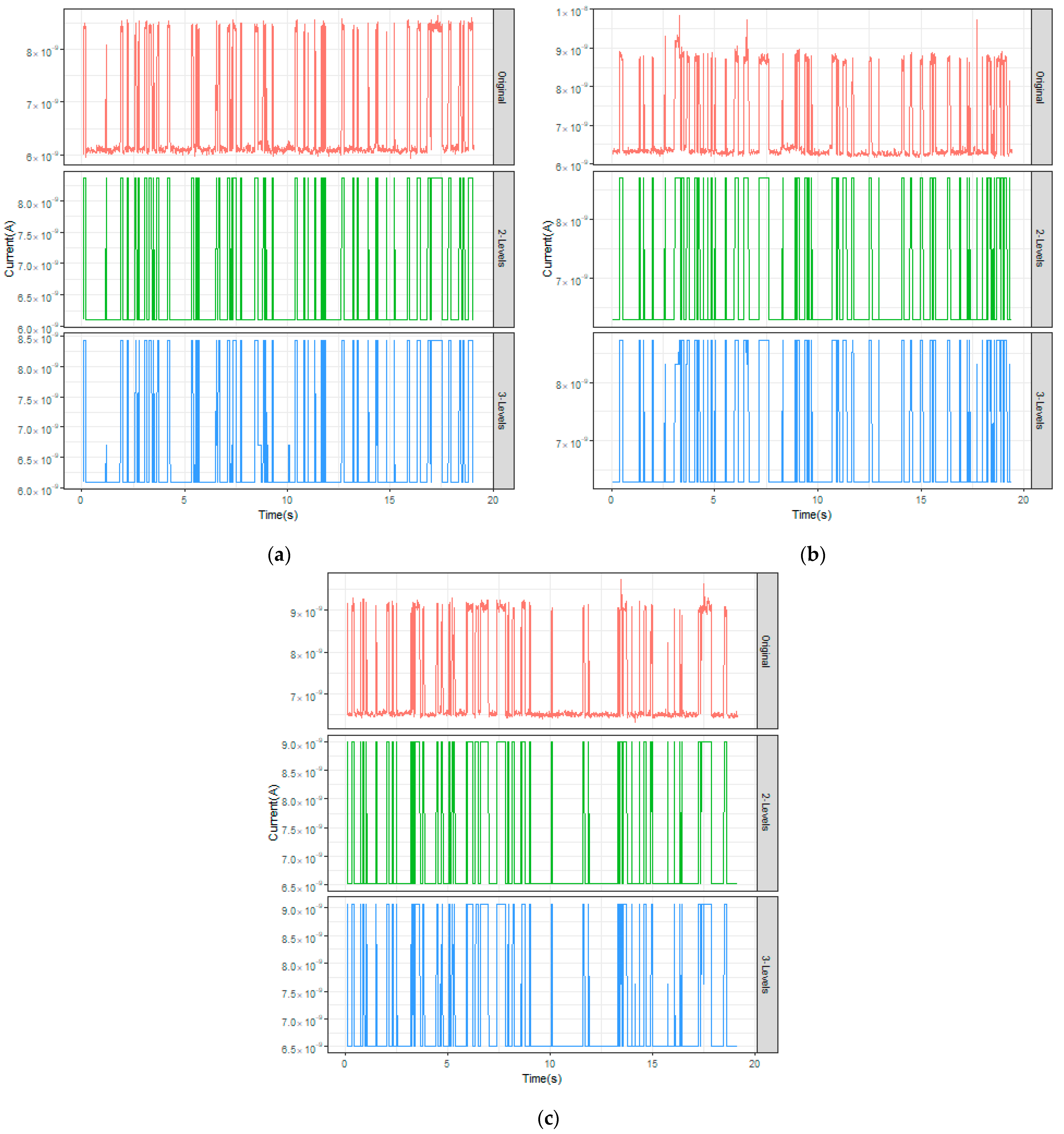
We analyzed different data sets for RTN25, RTN26, RTN27, and the hidden states from the corresponding signals were discriminated. The best fit was achieved for latent levels 2 and 3 for RTN25, RTN26, RTN27. Figure 2 shows the original observed RTN signals and the corresponding latent levels given by the model for both cases. This analysis was performed using the depmixS4 package of R-cran [28].

The RTN25/26/27 series was analyzed. The proportional number of times that the chain is in the latent states for the different proposed models is shown in

Table 1. Proportional number of times that each chain was in the latent states.

Signal	Model	Latent State 1	Latent State 2	Latent State 3
RTN25	2 latent states	0.784	---	0.216
	3 latent states	0.762	0.037	0.201
RTN26	2 latent states	0.756	---	0.244
	3 latent states	0.753	0.0305	0.2165
RTN27	2 latent states	0.7665	---	0.2335
	3 latent states	0.7575	0.0255	0.2170

.

For each model, the continuous Markov chain associated to the latent states was estimated, and the corresponding stationary distribution was achieved. This is shown in

Table 2. Stationary distribution for the different traces.

Signal	Model	Latent State 1	Latent State 2	Latent State 3
RTN25	2 latent states	0.7974	---	0.2026
	3 latent states	0.7847	0.0185	0.1968
RTN26	2 latent states	0.7708	---	0.2292
	3 latent states	0.7746	0.0165	0.2089
RTN27	2 latent states	0.7736	---	0.2264
	3 latent states	0.7785	0.0026	0.219

.

These values can be interpreted as the proportional time that the device is in each latent state in the stationary regime for the embedded continuous Markov chain. We observed that these values were very close to zero for the RTN25/26/27 devices. We tested this fact, and do not think it can be rejected.

Therefore, we assumed that the internal performance of the devices behaved as a Markov model with two latent states for the RTN25/26/27 traces. The Markov chains for two latent states for the different cases were estimated. The exponentiality of the sojourn time in each state cannot be rejected according to the p-values obtained by means of a Kolmogorov–Smirnov test, and the expected number of visits up to a certain time as explained in Section 4.1 also was estimated. These estimations are shown in

Table 3. Expected number of visits to each level for the different traces.

Signal	Level	t = 5	t = 10	t = 15	t = 20
RTN25	Level 1	12.3497	23.8609	35.3721	46.8833
	Level 2	11.5523	23.0635	34.5747	46.0859
RTN26	Level 1	12.8198	24.8162	36.8127	48.8092
	Level 2	12.0490	24.0455	36.0419	48.0384
RTN27	Level 1	11.5645	22.5305	33.4965	44.4626
	Level 2	11.7909	22.7569	33.7229	44.6890

.

6.2. Long RTN Trace

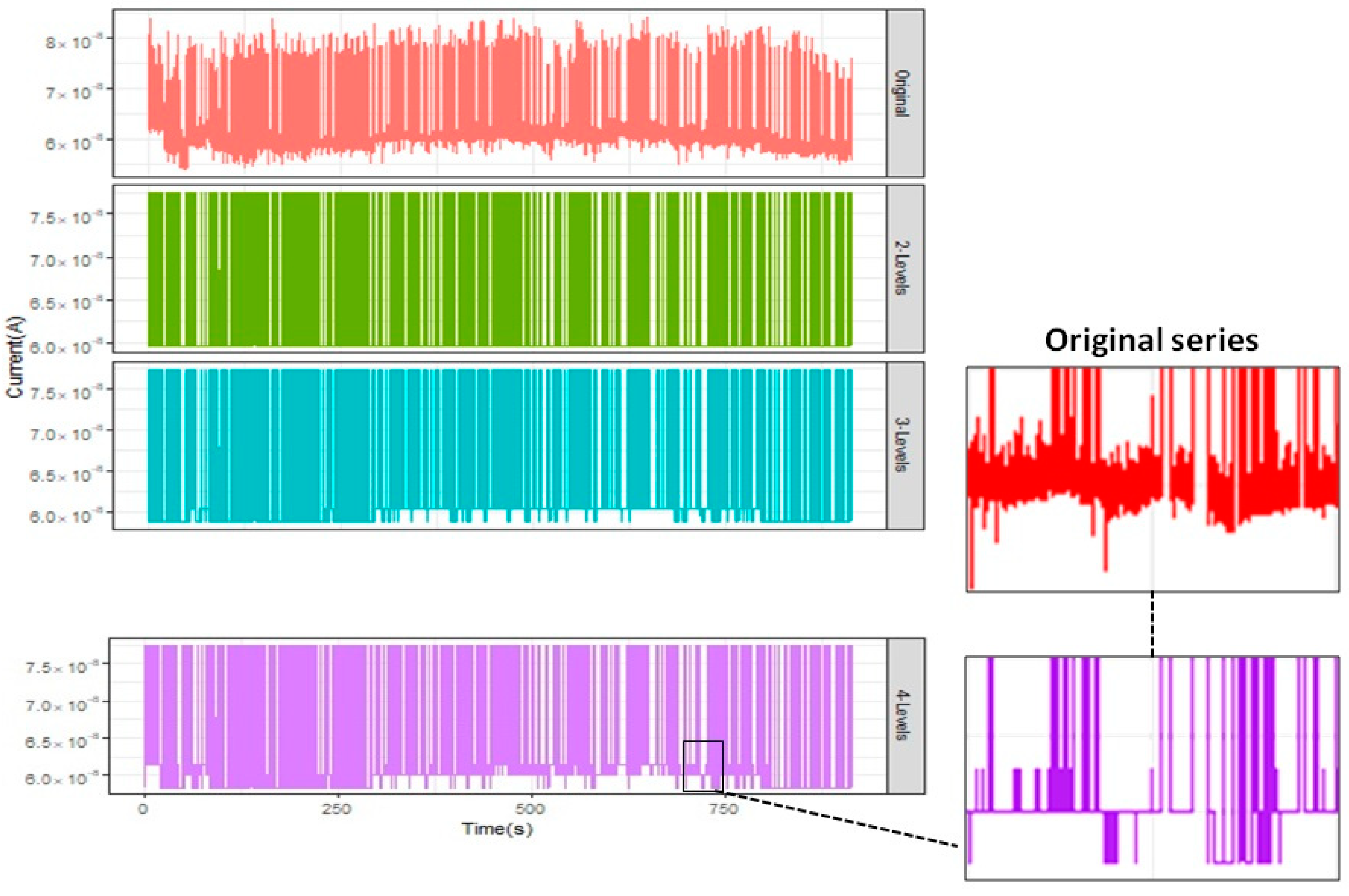
A similar exploratory analysis for this trace was carried out. This signal was supplied with 0.5 V, and its behavior was measured for more than three hours. To study the number of possible latent levels hidden in the signal, we again considered hidden Markov chains. The best fit was achieved for latent levels 3 and 4 for this long RTN trace. Figure 3 shows the original observed signal (a time interval of the whole signal was considered for the sake of computing feasibility) and the corresponding latent levels given by the model for both cases. This analysis also was performed using the depmixS4 package of R-cran.

We have focused on the four latent states. If the HMM is considered, the proportional time that the process was in each latent state was 0.3243048, 0.1219429, 0.1635429, and 0.3902095. If more latent states were assumed, negligible proportions would appear. Therefore, four different latent states were assumed. Before applying the new model to the data set, a statistical analysis was performed that considered classical techniques. For these latent states, the exponentiality of the sojourn time was tested and rejected through a Kolmogorov–Smirnov test for any latent state by obtaining the following p-values: 0.00027, 0.0045, 0.0000, and 0.0001, respectively. Next, we studied whether these times could be described as PH distributions. After multiple analyses, the best PH distributions for the latent states had 2, 2, 4, and 3 internal states, respectively. The structures of these PH distributions were generalized Coxian/Erlang distributions. Then, the internal behavior for each latent state passed across multiple internal states in a sequential way, one-by-one. The Anderson–Darling test was applied to test the goodness of fit, and obtained p-values of 0.8972, 0.4405, 0.0752, and 0.9876, respectively, for each latent state.

Generator of the Internal Markov Process

Given the previous analysis, we have observed that the sojourn time distribution in each macro-state (latent state) was phase-type distributed with a sequential degradation (generalized Coxian degradation). That is, the macro-states 1, 2 were composed of two phases (internal states), the macro-state 3 of four phases, and the macro-state 4 of three states. Thus, we assume the sojourn time in a macro-state i (level i) is PH distributed with representation $\left({\alpha }_i,T_i\right)$ with the following structure:

Macro-state 1	Macro-state 2
$\begin{array}{l}{\alpha }_1=\left({\alpha }_1^1,1-{\alpha }_1^1\right)\\ T_1=\left(\begin{array}{cc}-t_{12}^1& t_{12}^1\\ 0& -t_{13}^1\end{array}\right)\\ T_1^0=\left(0,t_{13}^1\right)’\end{array}$	$\begin{array}{l}{\alpha }_2=\left({\alpha }_1^2,1-{\alpha }_1^2\right)\\ T_2=\left(\begin{array}{cc}-t_{12}^2& t_{12}^2\\ 0& -t_{13}^2\end{array}\right)\\ T_2^0=\left(0,t_{13}^2\right)’\end{array}$
Macro-state 3	Macro-state 4
$\begin{array}{l}{\alpha }_3=\left({\alpha }_1^3,{\alpha }_2^3,{\alpha }_3^3,1-{\alpha }_1^3-{\alpha }_2^3-{\alpha }_3^3\right)\\ T_3=\left(\begin{array}{cccc}-t_{12}^3& t_{12}^3& 0& 0\\ 0& -t_{23}^3& t_{23}^3& 0\\ 0& 0& -t_{34}^3& t_{34}^3\\ 0& 0& 0& -t_{35}^3\end{array}\right)\\ T_3^0=\left(0,0,0,t_{35}^3\right)’\end{array}$	$\begin{array}{l}{\alpha }_4=\left({\alpha }_1^4,{\alpha }_2^4,1-{\alpha }_1^4-{\alpha }_2^4\right)\\ T_4=\left(\begin{array}{ccc}-t_{12}^4& t_{12}^4& 0\\ 0& -t_{23}^4& t_{23}^4\\ 0& 0& -t_{34}^4\end{array}\right)\\ T_4^0=\left(0,0,0,t_{34}^4\right)’\end{array}$

We assume that when the device leaves the macro-state i, it goes to macro-state j with a probability of p_ij, where p_ii = 0 and $p_{14}=1-{\displaystyle \sum _{i=1}^3{p}_{ij}}$, and the sojourn time in this new macro-state begins with the corresponding initial distribution α_j.

Thus, the behavior of the device is governed by a stochastic process {X(t); t ≥ 0} with an embedded Markov process {J(t); t ≥ 0}, as described in Section 2.1. The macro-state space is {1, 2, 3, 4} and the state space $\left\{1=i_1^1,2=i_2^1;3=i_1^2,4=i_2^2;5=i_1^3,6=i_2^3,7=i_3^3,8=i_4^3;9=i_1^4,10=i_2^4,11=i_3^4\right\}$.

In this case, the matrix blocks are $Q_{ii}=T_i$ and $Q_{ii}=p_{ij}{T}_i^0\otimes {\alpha }_j$ for i, j = 1,..., r and I ≠ j. Therefore, the matrix generator is given by:

$$Q=\left(\begin{array}{cccc}{T}_1& p_{12}{T}_1^0\otimes {\alpha }_2& p_{13}{T}_1^0\otimes {\alpha }_3& p_{14}{T}_1^0\otimes {\alpha }_4\\ p_{21}{T}_2^0\otimes {\alpha }_1& T_2& p_{23}{T}_2^0\otimes {\alpha }_3& p_{24}{T}_2^0\otimes {\alpha }_4\\ p_{31}{T}_3^0\otimes {\alpha }_1& p_{32}{T}_3^0\otimes {\alpha }_2& T_3& p_{34}{T}_3^0\otimes {\alpha }_4\\ p_{41}{T}_4^0\otimes {\alpha }_1& p_{42}{T}_4^0\otimes {\alpha }_2& p_{43}{T}_4^0\otimes {\alpha }_3& T_4\end{array}\right)$$

The parameters were estimated by considering the likelihood function built in Section 5. The estimated parameters with a value of the logL = −4066.118120 are:

$$P=\left(\begin{array}{cccc}0& 0.6667& 0.0407& 0.2926\\ 0.3870& 0& 0.1969& 0.4161\\ 0.0296& 0.2238& 0& 0.7466\\ 0.1605& 0.3395& 0.5& 0\end{array}\right)$$

$${\alpha }_1=\left(0.5730374,0.4269626\right);T_1=\left(\begin{array}{cc}-0.6790043& 0.6790043\\ 0& -4.1343018\end{array}\right)$$

$${\alpha }_2=\left(0.4699825,0.5300175\right);T_2=\left(\begin{array}{cc}-3.249849& 3.249849\\ 0& -10.426533\end{array}\right)$$

$${\alpha }_3=\left(0.0741494,0.4258142,0.5000364,0\right)$$

$$T_3=\left(\begin{array}{cccc}-0.5533471& 0.5533471& 0& 0\\ 0& -2.2755462& 2.2755462& 0\\ 0& 0& -29.535695& 29.535695\\ 0& 0& 0& -242.7465\end{array}\right)$$

$${\alpha }_4=\left(0.3593538,0.6406462,0.0000\right);T_4=\left(\begin{array}{ccc}-0.964899& 0.964899& 0\\ 0& -4.112655& 4.112655\\ 0& 0& -28.638854\end{array}\right)$$

Therefore, the generator of the Markov process {J(t); t ≥ 0} is:

$$\widehat{Q}=\left(\begin{array}{ccccccccccc}-0.6790& 0.6790& 0& 0& 0& 0& 0& 0& 0& 0& 0\\ 0& -4.1343& 1.2954& 1.4609& 0.0125& 0.0717& 0.0841& 0& 0.4347& 0.7750& 0\\ 0& 0& -3.2498& 3.2498& 0& 0& 0& 0& 0& 0& 0\\ 2.3122& 1.7228& 0& -10.4265& 0.1522& 0.8742& 1.0266& 0& 1.5590& 2.7794& 0\\ 0& 0& 0& 0& -0.5533& 0.5533& 0& 0& 0& 0& 0\\ 0& 0& 0& 0& 0& -2.2755& 2.2755& 0& 0& 0& 0\\ 0& 0& 0& 0& 0& 0& -29.5357& 29.5357& 0& 0& 0\\ 4.1174& 3.0679& 25.5326& 28.7941& 0& 0& 0& -242.7465& 65.1273& 116.1072& 0\\ 0& 0& 0& 0& 0& 0& 0& 0& -0.9649& 0.9649& 0\\ 0& 0& 0& 0& 0& 0& 0& 0& 0& -4.1127& 4.1127\\ 2.6340& 1.9625& 4.5696& 5.1533& 1.0618& 6.0974& 7.1602& 0& 0& 0& -28.6389\end{array}\right)$$

with initial distribution $\widehat{\mathsf{\theta }}=\left(0,0,0,0,0.0741494,0.4258142,0.5000364,0,0,0,0\right)$.

The stationary distribution was estimated for the process {X(t); t ≥ 0} (given in

Table 4. Stationary distribution for the process {X(t); t ≥ 0}.

	Level 1	Level 2	Level 3	Level 4
Selected interval in the long RTN trace	0.3273	0.1197	0.1612	0.3919

) from Section 2.2. It can be interpreted as the proportional time in each macro-state (long-run).

Finally, the mean number of visits to each macro-state up to a certain time t was obtained following Section 4.1. It is shown in

Table 5. Expected number of visits up to a certain time for different times.

Time	Level 1	Level 2	Level 3	Level 4
t = 50	16.0207	25.0716	20.3974	30.0827
t = 100	31.0837	49.9364	40.9591	60.1877
t = 200	61.1925	99.6404	82.0612	120.3666
t = 500	151.4018	248.5475	205.1981	300.6553

.

7. Conclusions

A real problem motivates the construction of a new stochastic process that accounts for the internal performance of different macro-states by considering that it follows an internal Markovian behavior. We have shown that the homogeneity and Markovianity was lost in the developed new macro-state model. The sojourn time in each macro-state was phase-type distributed depending on the initial observed time. The stationary distribution was calculated through matrix-algorithmic methods, and the distribution of the number of visits to a determined macro-state between any two different times was calculated using a Laplace transform. The mean number of visits depending on times was worked out explicitly.

The new developed methodology enables the modeling of complex systems in an algorithmic way by solving classic calculus problems. Thanks to the proposed development, the results and measures were worked out in an easier way and could be interpreted. Matrix analysis and Laplace transform techniques were used to determine the properties of the model, and algorithms to obtain quantitative results were provided. Given that everything was carried out algorithmically, is the model was implemented computationally and was successfully applied to study different random telegraph noise signals measured for unipolar resistive memories.

Resistive memory random telegraph noise signals were analyzed in depth in order to characterize them from a probabilistic point of view. These signals are essential, since they can pose a limit in the performance of certain applications; in addition, this type of noise can be good as an entropy source in the design of random number generators for cryptography. From the proposed model, we showed that a latent state of a resistive memory RTN long signal is composed of multiple internal states. Of course, the applications of a phase-type model, as given in this work, are not restricted to the RRAM context.