Article

Smooth Break Detection and De-Trending in Unit Root Testing

by
Furkan Emirmahmutoglu
1,
Tolga Omay
2,3,
Syed Jawad Hussain Shahzad
3,4,* and
Safwan Mohd Nor
5,6,*
1
Department of Econometrics, Ankara Haci Bayram Veli University, 06500 Ankara, Turkey
2
Department of Economics, Atilim University, 06830 Ankara, Turkey
3
Montpellier Business School, University of Montpellier, Montpellier Research in Management, 34080 Montpellier, France
4
Department of Accounting, Analysis and Audit, South Ural State University, 454080 Chelyabinsk, Russia
5
Faculty of Business, Economics and Social Development, University of Malaysia Terengganu, 21030 Kuala Nerus, Terengganu, Malaysia
6
Victoria Institute of Strategic Economic Studies, Victoria University, Melbourne, VIC 3000, Australia
*
Authors to whom correspondence should be addressed.
Mathematics 2021, 9(4), 371; https://doi.org/10.3390/math9040371
Submission received: 4 January 2021 / Revised: 4 February 2021 / Accepted: 8 February 2021 / Published: 13 February 2021
(This article belongs to the Special Issue Application of Mathematical Methods in Financial Economics)

Abstract

:
This study explores the methods to de-trend the smooth structural break processes while conducting the unit root tests. The two most commonly applied approaches for modelling smooth structural breaks namely the smooth transition and the Fourier functions are considered. We perform a sequence of power comparisons among alternative unit root tests that accommodate smooth or sharp structural breaks. The power experiments demonstrate that the unit root tests utilizing the Fourier function lead to unexpected results. Furthermore, through simulation studies, we investigate the source of such unexpected outcomes. Moreover, we provide the asymptotic distribution of two recently proposed unit root tests, namely Fourier-Augmented Dickey–Fuller (FADF) and Fourier-Kapetanios, Shin and Shell (FKSS), which are not given in the original studies. Lastly, we find that the selection of de-trending function is pivotal for unit root testing with structural breaks.

1. Introduction

Macroeconomic variables are subject to either smooth or sharp structural breaks e.g., great moderation since the mid-1980s or the 2007–09 global financial crisis. This led to the development of unit root tests allowing for different types of structural break. The unit root tests that employ a flexible Fourier function to model the structural breaks (Enders and Lee [1,2]) have attracted a great deal of attention compared to the tests employing the smooth transition (ST) function. In this paper, we show that the Fourier function may lead to an over-filtration problem when structural break and non-linearity are simultaneously present in the data. In particular, when we apply unit root tests that embed the Fourier function, we cannot identify whether the rejection of the unit root null is due to the presence of a structural break, state-dependent non-linearity, or both.
Structural changes in economic variables, which are affected by the heterogeneous behaviour of many economic agents, are more likely to follow a smooth, rather than an instantaneous, time path. Therefore, the smooth transition regression (STR), where parameters are assumed to change smoothly over time, became a realistic setup for modelling and testing structural changes [3,4]. To account for smooth breaks in the deterministic components of a time series, studies have developed alternative unit root tests based on Gallant’s [5] flexible Fourier form and the smooth transition (ST) method of Leybourne, Newbold and Vougas [6] (LNV). The main advantage of the Fourier approach is its ability to capture the behaviour of a deterministic function of unknown form even if the function itself is not periodic. In addition, it works better than dummy variable methods irrespective of whether the breaks are instantaneous or smooth [1]. Moreover, Fourier function avoids problems of selecting the dates, number and form of breaks [1,7]. Utilising the flexible Fourier form (FFF) has its own share of disadvantages. In particular, there is no unique way to selecting cumulative frequency components for the trigonometric functions. On the other hand, ST models estimate the parameters by using an appropriate non-linear estimation algorithm considering mean break, trend break or both, which gives extra important information about the composition of the structural break (see [8] for details). Moreover, the ST models are quite successful in modelling gradual or sharp structural breaks.
We also focus on the unit root tests that simultaneously allow for structural breaks (in the deterministic component) and state dependent non-linearity (in the stochastic component). Introducing both structural breaks and regime-switching behaviour into the testing framework is expected to deliver power gains compared to tests considering non-linearity or structural shift in isolation (see e.g., Christopoulos and Leon-Ledesma [9] (henceforth, CL or FKSS), and Omay and Yıldırım [10] (OY), among others). The recently developed FKSS and OY structural breaks unit root tests use the Fourier function and logistic smooth transition function in their testing strategy, respectively. To account for exponential smooth transition autoregressive (ESTAR) regime-wise nonlinearity, FKSS and OY have employed the Kapetanios, Shin and Snell [11] (henceforth, KSS) test in the second stage of their testing procedure.
Interestingly, our power analysis on the FKSS test, following same parameter specifications as in [1,2], show that Enders and Lee [2] (henceforth FADF) unit root test is superior. Notably, the power analysis conducted in Christopoulos and Leon-Ledesma [9] show that the FKSS test is superior to the FADF test. The better power performance was due to the symmetric or equal parameter values for the Fourier transforms’ components, namely sine and cosine. Symmetric values are very restrictive when we refer to the parameter specifications in [2]. Hence, the FADF captures all non-linearity (both time and state dependent non-linearity), may be an indication of over-filtration problem. Further, [1] claim that the LNV and KSS tests are alternatives to the FADF test. LNV test utilizes the smooth transition function in the deterministic component and thereby can be a potential rival of the FADF test. However, the KSS test, which includes an ESTAR type of non-linearity in its stochastic term, is a non-linear unit root test that assumes a non-linear speed of mean reversion and thus cannot be a potential alternative for the FADF. On the other hand, FKSS uses the Fourier function in its testing procedure, but imposes ESTAR non-linearity for the remaining part of the series. Therefore, FKSS supports that KSS test cannot be a potential alternate for the FADF test. FKSS considers FFF as a de-trending tool for detecting only structural breaks, but FADF considers FFF as a tool for detecting structural break and/or state-dependent non-linearity. Enders and Lee [1] also support their claim implicitly by using simulation analysis with low frequency k = 1 in order to capture different dynamics such as exponential smooth transition break, which is unusual break type in structural break literature. Furthermore, they analyse different types of smooth breaks and threshold autoregressive (TAR) type breaks.
Enders and Lee [1] conclude that FFF can imitate a large variety of structural breaks (or functions with low frequency components). They allow for only the structural break in their testing procedure, and do not consider the interaction between the structural breaks and non-linear stochastic components. Their claim that the KSS test is a rival of their testing procedure can still be understood when the results of their simulation experiments on different functional forms are considered. From their simulation experiments, it can be seen that the Fourier function can also imitate any kind of series’ structure as well as state-dependent non-linearity by using the low-frequency component, but this phenomenon is not explained explicitly in their study. The Fourier function is extensively studied in continuous form in the applied and theoretical mathematics literature. To consider all the aforementioned issues, we first concentrate on the unit root tests which use the Fourier function. Then, we use the smooth transition function to understand the behaviour of the Fourier function in more complex data-generating processes (DGP). Moreover, we have also included other testing procedures to compare and contrast the behaviour of different functions in different DGPs.
We start the power analysis by first using the FKSS-DGP. The Enders and Lee [2] (henceforth EL) test is found to have better power performance than the FKSS unit root test in this DGP setting. This contradiction is the main concern of our paper that the FFF methodology has some over-filtration problem while detecting the structural break even with its low frequency component k = 1 . To elaborate more on this issue, we proceed with the KSS-DGP, because the KSS test is claimed to be the alternative of the EL test. The best performing test in a KSS-DGP setting is found to be the FKSS test, which is again an unexpected result. In the original work of the KSS, except some of the parameter region (where the ADF test power superior to other alternatives) best performing test is their test. On the other hand, if we consider the Enders and Lee [1] claim, then power analysis might exhibit better power performance of EL test. However, FKSS test has better power performance in a state-dependent non-linear DGP with its two components, the FFF and ESTAR non-linearity. This unexpected result is further investigated in the simulation analysis. Moreover, since the LNV test is also considered as one of the alternatives to the EL test, the LNV-DGP is also used for the power analysis. This power experiment shows that the FKSS test’s power performance exceeds that of the EL test; however, the LNV is still the best test in its DGP, which is an expected result. As the fourth and last candidate, OY-DGP is taken into consideration which uses structural break (logistic smooth transition) and non-linearity (ESTAR) simultaneously. The OY test can be seen as an alternative test to the FKSS test which uses logistic smooth transition function as a tool for detecting structural break instead of FFF. Again, we witness that the power performance of the FKSS is better than that of the EL test, but the most powerful test is the OY test in this DGP, as expected. The results of all these power experiments are discussed in detail in the fourth section. (We have also conducted the additional simulation exercises in the Technical Annex, which also supports the general conclusion of the current paper.) These exercises give important clues for identifying the true modelling strategy of the structural breaks.
Now, we are left with one interesting question. Is there any degree of resemblance between the STR type and FFF type of de-trending? To answer this question, the simplest way is to generate a Fourier-type non-linear trend and approximate it with a STR type of de-trending. This method is the opposite of what reference [1] have done in their paper. They generated STR- and TAR-type non-linear trends and approximated them with Fourier type de-trending. In this paper, by using STR-type de-trending, we approximate FFF type of de-trending. By using this inverse methodology, we can determine the transition speed of FFF. These simulation studies show that the STR type of de-trending can imitate sharp breaks as well as smooth breaks as expected. Therefore, it can be concluded that the STR type of de-trending is more flexible than the Fourier transforms in capturing the one structural break. However, the Fourier transforms have an advantage over the STR de-trending in that they can be applied in the case of more than one smooth structural break.
The rest of the paper is structured as follows: Section 2 describes the alternative testing procedures and give the asymptotic distribution of the FADF and FKSS tests, since they are not given in the original studies. Section 3 examines and compares the small sample power performance of these tests in the context of the linear and non-linear unit root tests. (We have also conducted substantial simulation studies in order to deal with anomalies obtained in power analysis, which are not reported but can be given upon request.) We provide two empirical illustrations in Section 4. Section 5 concludes.

2. The Unit Root Tests and their Testing Frameworks

2.1. FADF-FKSS Tests and their Asymptotic Distributions

Let us consider the following data generating process:
y t = α 0 + α 1 t + φ 1 s i n ( 2 π k t T ) + φ 2 c o s ( 2 π k t T ) + x t ,   t = 1 ,   , T
where k denotes the integer Fourier frequency. Moreover, φ 1 and φ 2 measure the amplitude and displacement of the sinusoidal component of the deterministic term. Prior studies [1,2,7,9,12,13] suggest that Fourier transforms will often lead to a good approximation to a model with structural breaks. Following these studies, we allow a single Fourier frequency in Equation (1). They observe that a single Fourier frequency can mimic a large variety of breaks in the deterministic trend function. However, [1] demonstrate that the presence of many frequency components uses degrees of freedom and can lead to an over-fitting problem.
Remark 1.
The deterministic components given in Equation (1) include a linear time trend. However, we may also consider the case where only a constant and the Fourier terms are contained, which it is α_1 = 0 in Equation (1). This will be referred to as the demeaned case in what follows, while the more general case where α_1 ≠ 0 will be termed the detrended case.
In the above Equation (1), we assume that x t has the following two stochastic processes:
x t = ϕ x t 1 + u t
x t = ϕ x t 1 + γ x t 1 [ 1 e x p ( θ x t d 2 ) ] + u t
where u t ~ i i d ( 0 , σ 2 ) and the initial condition x 0 is zero. Equation (2) represents a standard Dickey–Fuller (DF) regression that assumes linear adjustment toward equilibrium. However, Equation (3) assumes that the adjustment speed is nonlinear and follows an ESTAR process developed in KSS [11].
In this study, we propose the two-step testing procedure like CL [9]. In the first step, we obtain the demeaned or detrended series, x ˜ t say.
x ˜ t = y t α ^ 0 φ ^ 1 s i n ( 2 π k t T ) φ ^ 2 c o s ( 2 π k t T )       f o r   d e m e a n e d   c a s e x ˜ t = y t α ^ 0 α ^ 1 t φ ^ 1 s i n ( 2 π k t T ) φ ^ 2 c o s ( 2 π k t T )       f o r   d e t r e n d e d   c a s e
where α ^ 0 , α ^ 1 , φ ^ 1 and φ ^ 2 are OLS estimators. Next, we construct two Fourier based unit root test with x ˜ t in the second step. Firstly, we consider the Dickey-Fuller type unit root test. The DF Equation in (2) can be re-written as:
Δ x ˜ t = β x ˜ t 1 + e t
where β = ϕ 1 and e t ~ i i d ( 0 , σ e 2 ) . We are interested in testing the null hypothesis of unit root ( β = 0 ) against the stationary alternative ( β < 0 ) in Equation (4). Relaxing the assumption that e t are serially uncorrelated, Equation (4) can be written by augmenting with sufficient lags of the dependent variable as follows:
Δ x ˜ t = β x ˜ t 1 + j = 1 p δ j Δ x ˜ t j + e t
Then the test for the null hypothesis β = 0 against the alternative β < 0 is obtained with the following t-statistics:
t i F A D F = β ^ s . e . ( β ^ )                     i = μ , τ
where β ^ and s . e . ( β ^ ) are the OLS estimate and associated standard error of β obtained from Equation (5). Secondly, we examine the ESTAR-type unit root test. Equation (3) can be reparametrized with x ˜ t instead of x t as follows:
Δ x ˜ t = β x ˜ t 1 + γ x ˜ t 1 [ 1 e x p ( θ x ˜ t d 2 ) ] + e t
where β = ϕ 1 . KSS assume that d = 1 , and that γ < 0 and γ + β < 0 ( β 0 is possible) for globally stationary process. After imposing β = 0 , we can write Equation (7) as:
Δ x ˜ t = γ x ˜ t 1 [ 1 e x p ( θ x ˜ t d 2 ) ] + e t
We follow KSS and consider the null hypothesis, H 0 : θ = 0 in Equation (8), under which x ˜ t is non-stationary unit root. Notice under the null that the parameter θ is not identified. Thus, we follow KSS [11] and Luukkonen et al. [14], and adopt the first-order Taylor expansion of G ( x ˜ t d ; θ ) around θ = 0 with d = 1 . KSS derive the auxiliary testing regression as follows:
Δ x ˜ t = δ x ˜ t 1 3 + η t
where η t = e t + R t with R t representing the remainder terms from the Taylor expansion and δ = θ γ . If residuals η t are serially correlated, Equation (9) can be extended to correct for the serial correlation as:
Δ x ˜ t = δ x ˜ t 1 3 + j = 1 p ω j Δ x ˜ t j + η t
Thus, we can obtain the t statistics for δ = 0 against δ < 0 as follows:
t i F K S S = δ ^ s . e . ( δ ^ )               i = μ , τ
where δ ^ is the OLS estimator of δ in Equation (10) and s . e . ( δ ^ ) is the standard error of δ ^ .
To obtain the asymptotic distribution of the t i F A D F and t i F K S S ( i = μ , τ ) statistics, we need the following results, where we let [ r T ] , r [ 0 , 1 ] , be an integer close to r T . Throughout the paper, signifies weak convergence as T approaches .
Proposition 1.
i T 3 / 2 t = 1 T x t σ 0 1 W ( r ) d r = σ f 1
ii T 5 / 2 t = 1 T t x t σ 0 1 r W ( r ) d r = σ f 2
iii T 3 / 2 t = 1 T s i n ( 2 π k t T ) x t σ 0 1 s i n ( 2 π k r ) W ( r ) d r = σ f 3
iv T 3 / 2 t = 1 T c o s ( 2 π k t T ) x t σ 0 1 c o s ( 2 π k r ) W ( r ) d r = σ f 4
v 1 T t = 1 T sin ( 2 π k t T ) 0
vi 1 T t = 1 T cos ( 2 π k t T ) 0
vii 1 T 2 t = 1 T t sin ( 2 π k t T ) 1 2 π k
viii 1 T 2 t = 1 T t cos ( 2 π k t T ) 0
ix 1 T t = 1 T sin 2 ( 2 π k f t T ) 0.5
x 1 T t = 1 T cos 2 ( 2 π k t T ) 0.5
xi 1 T t = 1 T sin ( 2 π k t T ) cos ( 2 π k t T ) 0
Theorem 1.
The test statistics given in Equations (6) and (11) under the null have the following asymptotic distributions:
t i F A D F d 0 1 W i ( k , r ) d W ( r ) ( 0 1 W i ( k , r ) 2 d r ) 1 / 2                     i = μ , τ t i F K S S d 0 1 W i ( k , r ) 3 d W ( r ) ( 0 1 W i ( k , r ) 6 d r ) 1 / 2                     i = μ , τ
where W ( r ) is the Wiener process as defined over the interval r [ 0 , 1 ] . W i ( k , r ) for i = μ , τ is demeaned and detrended Brownian motion, respectively.
Proof. 
See the Appendix A. □
Obviously, the asymptotic distribution of the resulting test statistics under the null depends on the Fourier frequency k , but invariant to other parameters in the model. Table 1 gives asymptotic critical values of the t i F A D F and t i F K S S statistics for different values of k . These values are obtained from numerical simulations where the Wiener process is approximated by partial sums of 2000 independent N ( 0 , 1 ) variates and the number of replications is 100,000.

2.2. Unit Root Tests with Alternative Smooth Transition Type Break

Next, we introduce and describe the three other tests, which use the logistic smooth transition function. They are the tests proposed by [6,10,15]. Suppose that y t follow a smooth transition trend function on the time domain,   t = 1 , 2 , , T :
y t = α 01 + α 2 S t ( λ , τ ) + ε t
y t = α 0 + β 1 t + α 2 S t ( λ , τ ) + ε t
y t = α 0 + β 1 t + α 2 S t ( λ , τ ) + β 2 t S t ( λ , τ ) + ε t
where ε t is a zero mean stationary process and S t ( λ , τ ) is the logistic smooth transition regression (STR) function.
S t ( λ , τ ) = [ 1 + e x p { λ ( t τ T ) } ] 1 ,     λ > 0
Here, the structural change is assumed to follow a smooth transition between regimes rather than an instantaneous structural break. S t ( λ , τ ) is a continuous function bounded between 0 and 1. The STR can be the interpreted as a regime-switching model between the two extreme values of S t ( λ , τ ) = 0 and S t ( λ , τ ) = 1 , which allows the transition from one regime to the other is gradual. The parameter, λ determines the smoothness of the transition. The two regimes are associated with small and large values of the transition variable, s t = t relative to the threshold, c = τ . For the large values of λ , S t ( λ , τ ) passes through the interval ( 0 , 1 ) very rapidly. As λ approaches + , this function changes from 0 to 1 instantaneously at t = τ T . Therefore, y t in Model 1 is a stationary process around a mean changing from α 1 to α 1 + α 2 .
In these specifications, no change and one instantaneous structural change are limiting cases. LNV [6] propose a two-step procedure:
  • Step 1: We first estimate the deterministic component of the respective model by applying a Nonlinear Least Squares (NLS), and construct the residuals:
    Model 1: ε ^ t = y t α ^ 0 α ^ 2 S t ( λ ^ , τ ^ )
    Model 2: ε ^ t = y t α ^ 0 β ^ 1 t α ^ 2 S t ( λ ^ , τ ^ )
    Model 3: ε ^ t = y t α ^ 0 β ^ 1 t α ^ 2 S t ( λ ^ , τ ^ ) β ^ 2 t S t ( λ ^ , τ ^ )
  • Step 2:
    (i)
    Using an ADF test in the second step leads to the Leybourne et al. [6] LNV unit root test.
    (ii)
    Using an EG unit root test in the second step leads to the Sollis [15], S unit root test.
    (iii)
    Using a KSS test in the second step leads to the Omay and Yıldırım [10], OY unit root test.

3. The Finite Sample Performances

In this section, we consider the number of DGP, which are designed to simultaneously model structural breaks and regime-dependent non-linearities, in order to compare the finite sample performances of the alternative estimators reviewed in Section 2.

3.1. The Fourier-Exponential Smooth Transition Autoregressive (ESTAR) Hybrid Data-Generating Processes (DGP)

We first investigate the empirical power of the tests by using the FKSS-DGP where the process is a stationary nonlinear adjustment around a smooth break. We construct the Fourier-ESTAR(1) model by:
y t = φ 1 s i n ( 2 π k t T ) + φ 2 c o s ( 2 π k t T ) + ε t
Δ ε t = γ ε t 1 [ 1 e x p ( θ ε t 1 2 ) ] + η t KSS   1 s t   DGP Δ ε t = ψ ε t 1 + γ ε t 1 [ 1 e x p ( θ ε t 1 2 ) ] + η t KSS   2 n d   DGP
where η t ~ i i d N ( 0 , 1 ) and φ 1 and φ 2 are the parameters of the Fourier series and take the values { 0.0 , 3.0 } and { 0.0 , 3.0 , 5.0 } , respectively. We also consider the following parameter values: for γ = { 0.1 , 1.0 , 1.5 } , for the transition speed, θ = { 0.01 , 1.0 } , k = 1 and ψ = 0.1 . These simulation results for T = 100 are presented in Table 2.
LNV state that the natural competitor of Model 1 (including the structural break in the intercept only) is the ADF test which includes both intercept and trend. Since the original KSS and ADF tests do not allow for a structural break, we include both terms in our power analysis. As readily seen from Table 2, the power of the EL test dominates all other tests. This result is rather unexpected, because the power of the FKSS test is expected to dominate mostly under the current DGP, except for the parameter region where the transition parameter θ is sufficiently high. A general finding by KSS and OY suggests that non-linear unit root tests are relatively more powerful when the slope parameter is relatively small regardless of the values of γ . But, their power falls as the slope parameter rises. If the slope parameter is equal or greater, the power of the Dickey–Fuller test dominates other tests. Notice that as θ grows large, the model becomes approximately linear, though θ is not a scale-free parameter. KSS [11] argue that the nonlinear tests would be more powerful than the linear tests in the region local to the null, where the series tends to be more persistent. They state that most economic time series are likely to be highly persistent or stay near unit root. Thus, we argue that the power results tabulated in Table 2 are not in line with the findings by KSS and OY.
Enders and Lee [1] claim that the LNV and KSS tests deal with smooth structural breaks in their unit root testing procedures, via LSTR and ESTR breaks, respectively. Notice however that the KSS test is a non-linear unit root test that imposes the ESTR non-linearity to the stochastic component of the series, but it does not deal with structural breaks directly. As argued by Becker et al. [12], the presence of high-frequency components would reflect various forms of stochastic parameter instability. In this regard, we argue that the non-linearity embedded within the KSS test would be regarded as dealing with the stochastic parameter instability instead of smooth deterministic structural breaks.
Originally, the EL test was proposed for smooth structural break. EL argue that the low-frequency component of the Fourier function only captures the smooth structural break. However, the power analysis employed here with this hybrid data sheds light on the issue that the low-frequency component also captures non-linearity in the stochastic component which can be classified as stochastic parameter instability. As previously stated, the presence of high-frequency components would reflect various forms of stochastic parameter instability such as non-linearity in the slope parameter of the ESTAR type of unit root test. Therefore, using low-frequency component k = 1 it is not feasible to capture such a parameter’s instability. Notice that we consider the low-frequency ( k = 1 ) component only, in the power analyses reported in Table 1. However, the EL test has the best-performing test in this DGP setting. Enders and Lee [1,2] probably recognise that the low frequency Fourier approximation ( k = 1 ) filters out structural breaks as well as other forms of non-linearity, as discussed in the Introduction. Due to this observation, they classify the KSS test as the alternative to their unit root test. In the current setting, two sources of non-linearity are imposed (smooth structural break and state-dependent non-linearity) and the EL test captures both of them. This result seems to be in contradiction with Becker et al. [12] and Enders and Lee [1]. Therefore, aggregating the results of power analysis tabulated in Table 3 with the findings in the related literature, we can conclude that the low-frequency component of the Fourier function over-filters the hybrid DGPs or it can capture both smooth break and non-linearity in stochastic parts.
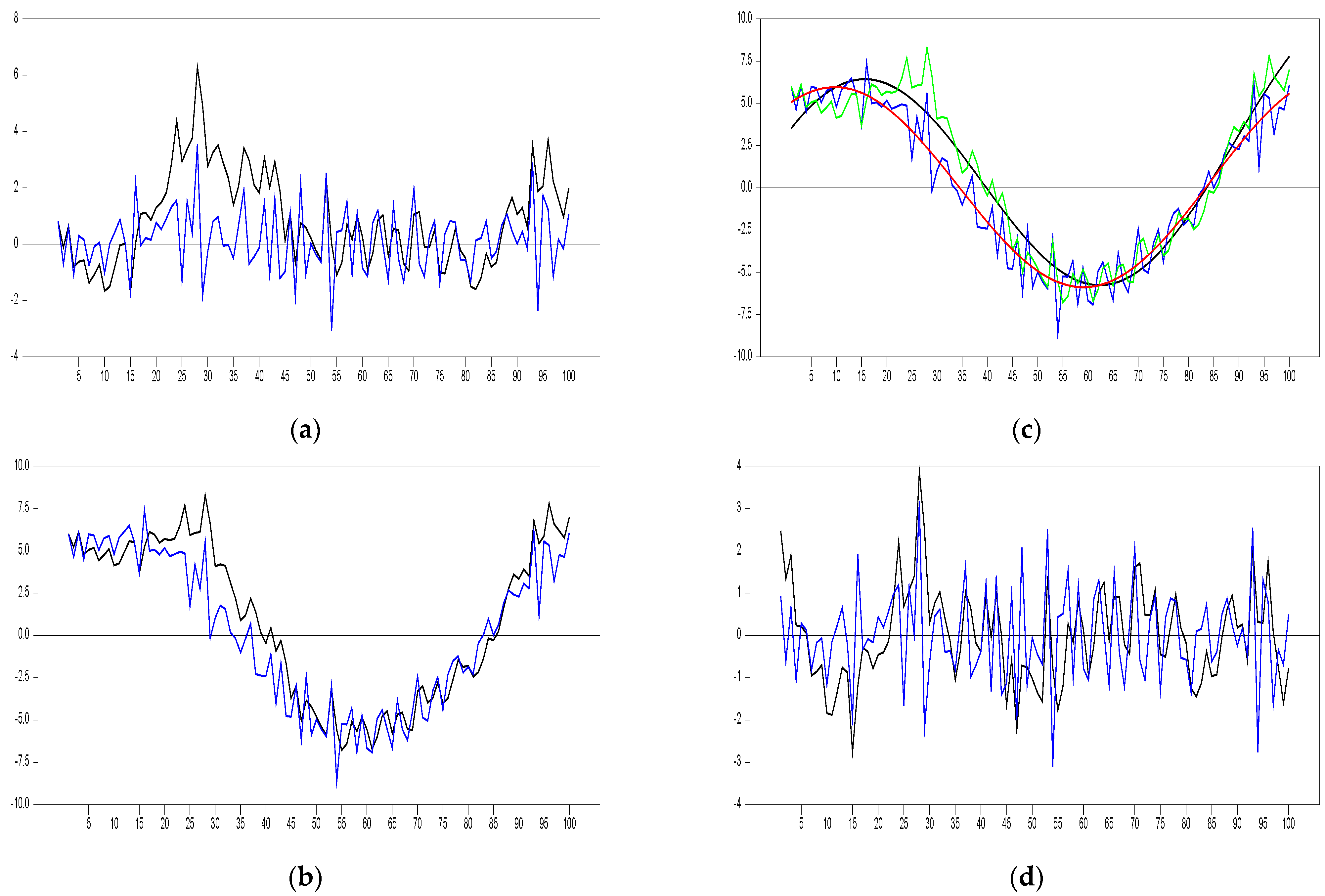
It may be useful to further prove the over-filtration problem of Fourier transforms in hybrid DGP by employing a newly designed simulation study. Figure 1 is generated under the two sets of DGP. The first is the linear A R ( 1 ) process with the AR parameter, 0.8 (light series), and the other is the KSS DGP with θ = 0.01 and γ = 1.5 (dark series). We can explicitly see the difference between linear and non-linear series in Panel (a) of Figure 1. In Panel (b), the two DGPs augmented with the same Fourier series ( φ 1 = 3.0 and φ 2 = 5.0 ) are displayed; they are the F ( k = 1 ) A R ( 1 ) process (Fourier trend with k = 1 plus an A R ( 1 ) ), and the F ( k = 1 ) E S T A R ( 1 ) process, respectively. In Panel (c) the non-linear trends estimated using the Enders and Lee [1,2] methodology. Therefore, we expect to obtain the same Fourier trends from both series y ^ t F T = α 0 + 3.0 s i n ( 2 π k t T ) + 5.0 c o s ( 2 π k t T ) . We obtained the same Fourier trend y ^ t F T from F ( k = 1 ) A R ( 1 ) DGP, however, the estimated Fourier trend from F ( k = 1 ) E S T A R ( 1 ) is not equal to y ^ t F T . When we have obtained the residuals from de-trended series from F ( k = 1 ) A R ( 1 ) and F ( k = 1 ) E S T A R ( 1 ) in Panel (d) of Figure 1, we see that estimated Fourier trend from F ( k = 1 ) E S T A R ( 1 ) is equal to the summation of two effects:
y ^ t F T α 0 + 3.0 s i n ( 2 π k t T ) + 5.0 c o s ( 2 π k t T ) + γ ε t 1 [ 1 e x p ( θ ε t 1 2 ) ]
Therefore, when we de-trend F ( k = 1 ) E S T A R ( 1 ) by using the Fourier k = 1 we are left an A R ( 1 ) process with approximately the AR parameter, 0.8. (More specific, Δ ε t = ψ ε t 1 + γ ε t 1 [ 1 e x p ( θ ε t 1 2 ) ] + η t , KSS 2 nd DGP with ψ = 0.8 ).
In Figure 1, Panel (a), the blue series is an AR(1) stationary process while the black series is the stationary ESTAR (1) process. In Panel (b), the same Fourier function has been added to these two processes with the same colours. In Panel (c), trend functions were found using the grid search method described in Enders and Lee [1] in these two series. The Red Fourier trend is obtained for AR (1)+Fourier and Black Fourier trend is obtained for ESTAR (1)+Fourier. Finally, we can see the nonlinear detrended ESTAR (1) process and AR(1) processes in Figure 1, Panel (d). As can be seen from here, the Fourier de-trended stationary AR(1) process given in blue is the same as the Fourier de-trended ESTAR(1) process given in black, which has almost transformed into the same structure.
We now provide more explanations about the behaviour of the Fourier series. (The convergence of the Fourier transforms to a stochastic process is studied by Gallant [5]. He argued that the norm measure shall be global and the Sobolov norm satisfies these requirements. See Technical Annex for more details, which is available upon request.) We first have the Dirichlet (1829) condition, stating that the Fourier series converge to a real-valued periodic function at every jump discontinuity from its midpoint [17]. Furthermore, it is well-established that as the frequency component increases, the low frequencies capture the structural break or deterministic components of the series whilst the high-frequency components capture the other stochastic component (e.g., [5,12,18,19,20]). These can be combined to explain unexpected findings in the power analysis observed in Table 2. When estimating a stochastic process with Fourier series, the low-frequency estimates the mid-point of the highest jump discontinuity, which we call a structural break (see also [1,2]). This issue can also be traced from Figures 1 and 3 in [13]. Therefore, the second series generated under the ( F ( k = 1 ) E S T A R ( 1 ) ) leads to a bigger jump discontinuity in Panel (b). Thus, in the estimation phase in Panel (c) the Fourier function passes through the mid-point of this jump discontinuity, however this jump discontinuity is now obtained by two different sources (smooth structural break and state-dependent non-linearity). Therefore, in Panels (c) and (d), we see that the Fourier trend overreact to ( F ( k = 1 ) E S T A R ( 1 ) ) DGP due to the Dirichlet condition where this result contradicts with [1,2,5,12,18,19,20].
To further support our claim of the over-filtration of the Fourier transforms, we conduct the following simulation experiment. First, we construct the FKSS-DGP similarly to the power analysis conducted in Table 2. Next, we estimate structural break by the Fourier function and then test the ESTAR non-linearity with the de-trended series. This simulation study can be used as the validation of the results in Figure 1. Here we employ the linearity test proposed by [14]. Notice that the KSS test is the linearized version of the first order Taylor approximation of the ESTAR non-linearity.
From the first row of Table 3, we find that 180 out of 2000 (9%) simulated series exhibit non-linearity by the LM test. The simulated series are ( F ( k = 1 ) E S T A R ( 1 ) ) series, therefore after removing the Fourier trend y ^ t F T , we expect to obtain ESTAR-type non-linearity from de-trended series. The LM test is employed to the de-trended series; however, the non-linearity obtained in these de-trended series does not exceed 17.5% which means that state-dependent non-linearity has disappeared.
This simulation experiments further confirm the power analysis in Table 3 and explanation obtained from Figure 1. Therefore, the estimated Fourier trends are as follows:
y ^ t F T α 0 + φ 1 s i n ( 2 π k t T ) + φ 2 c o s ( 2 π k t T ) + γ ε t 1 [ 1 e x p ( θ ε t 1 2 ) ] y ^ t F T α ˜ 0 + φ 1 s i n ( 2 π k t T ) + φ 2 c o s ( 2 π k t T )
φ 1 and φ 2 includes the features of γ ε t 1 [ 1 e x p ( θ ε t 1 2 ) ] and the de-trended series are A R ( 1 ) process. Thus, we obtain very rare rejection of null hypothesis of linearity.

3.2. The Behaviour of the Fourier Function under the Exponential Smooth Transition DGP

As mentioned in the Introduction, the KSS test is one of the potential rivals of the EL test and our previous results (in Table 2 and Table 3, and Figure 1) also support the claim of [1,2]. Therefore, it is interesting to see the power performance of the EL test under the KSS-DGP setting as that may increase our understanding of the behaviour of the Fourier function for state-dependent non-linearity in isolation. We now consider the following E S T A R ( 1 ) process as a DGP:
Δ y t = γ y t 1 [ 1 e x p ( θ y t 1 2 ) ] + η t
where we use γ = { 0.1 ,   1.0 ,   1.5 } and θ = { 0.01 ,   1.0 } . The power experiments obtained under this DGP with T = 100 are summarized in Table 4.
We find from Table 4 that the most powerful test appears to be the CL Test, t μ F K S S . This is rather an interesting result, considering the claim by Enders and Lee [1] that “If a non-linear trend is absent from the DGP, a standard unit root test without a non-linear trend will be more powerful than our test.” Even in the region where the KSS test should be mostly powerful, we find that the CL test performs better than the KSS test. The KSS test is constructed after deriving the Taylor approximation to the original ESTAR process; hence some information inherent in the data may be lost. Thus, the Fourier function incorporated in the KSS test would make some adjustments for the remainder of the terms ( R t ), thereby increasing the power of the CL test and showing why a non-linear unit root test including Fourier transforms displays better power even under the DGP without containing any structural breaks. On the other hand, the EL test has similar power to the KSS test as a second-best test. This result again supports the findings that we have found in the previous section and the claim of [1,2]. This result is also an indication of the over-filtration problem of the Fourier function, showing that the Fourier function can imitate any type of series behaviour even if it has a low-frequency component k = 1 while de-trending the series.
By using the KSS DGP, we have reached the conclusions given above, but the KSS DGP has its own limitation to show more information about the behaviour of the Fourier function. The transition speed θ is taken to be 0.1 and 1.0; these are of relatively smooth transition speed, hence for further investigation we have to increase the transition speed in order to see the behaviour of Fourier function. However, when we increase the θ greater than 1, the power results of all tests rapidly converge to 1.0. Therefore, there is no opportunity to compare the unit root test with each other and the behaviour of the Fourier function. Thus, for a moderate and sharp transition, it is better to select the DGP setting where we can provide these kinds of features. As mentioned earlier, the second potential rival test for the EL test is the LNV test. The LNV test is simply the logistic smooth transition counterpart of the EL test which is also proposed for detecting smooth structural breaks. Therefore, we proceed with the LNV-DGP in the next section in order to see the behaviour of the Fourier function in sharp transitions and/or sharp breaks.

3.3. The Behaviour of the Fourier Function under the Logistic Smooth Transition DGP

We proceed to conduct the power experiment under the DGP set-up by the LNV test, which is an important alternative to the EL test. This contains the logistic smooth transition function (LST), which has desirable features in determining the location of the structural break and speed of transition. The speed of transition parameter, λ determines the structure of breaks such that smooth and sharp breaks are dictated by low and high values, respectively.
We construct the following S T R A R ( 1 ) DGP, in which there is a stationary nonlinear adjustment around a smooth transition from one constant to another:
y t = α 1 + α 2 S t ( λ , τ ) + ε t S t ( λ , τ ) = [ 1 + e x p { λ ( t τ T ) } ] 1 ,       λ > 0 Δ ε t = δ ε t 1 + η t ,             η t ~ i i d ( 0 , 1 )
Here, S t ( · ) is a logistic smooth transition function, and we consider of the following parameter values: for the speed of transition parameter, λ = { 0.1 ,   0.2 ,   0.5 ,   0.7 ,   1.0 ,   2.5 ,   5.0 ,   10.0 } , for the threshold parameter, τ = { 0.2 ,   0.5 } and for the structural break parameter, α 2 = { 2.0 ,   5.0 ,   10.0 } (small, medium and large breaks), and for the autoregressive parameter, δ = 0.8 . These results with T = 100 are provided in Table 5.
In Table 5, we consider three different cases depending on the magnitudes of the structural break parameter α 2 . For the small break with α 2 = 2.0 , the ADF test performs better than all the other tests, see also similar results documented in LNV, Sollis [15] and OY. Surprisingly, however, the second-best test in this parameter region is the EL test, not the LNV. This may simply reflect that the Fourier form performs better in approximating the very smooth breaks. (The CL test is as good as the other test and better than the STR type analogous test LNVKSS (OY test). The FKSS test is better than the OY test, with the reason similar to the comparison of LNV and the EL test.) The power of all the tests is negatively associated with the λ parameter. Furthermore, the threshold location parameter, τ , also affects the power of the STR-type tests negatively. In particular, when the threshold is located at the beginning of the sample, the Fourier type tests tend to display better power, see [12] for similar findings. They document that the power of the Fourier type structural break test (i.e. the Trig-test) deteriorates as the break point moves to the end of the sample.
For the moderate structural break with α 2 = 5.0 , we obtain completely different results. For small slope parameters with the structural break dated at the beginning of the sample, ( τ = 0.2 ) the ADF test outperforms all the other tests. As the slope parameter λ rises, the CL test becomes more powerful. This result is somewhat unexpected. On the other hand, when the structural break parameter is located in the middle of the sample ( τ = 0.5 ), the ADF test performs best for the low values of λ only. As expected, in the rest of the parameter region, the LNV test becomes more powerful than the other tests. Hence, we may conclude that the logistic smooth transition function is able to capture the sharper breaks.
The Fourier-type structural break unit root tests are shown to display better power performance when the structural break is located at the beginning of the sample. Thus, a unit root test such as the EL test, that includes Fourier transforms, is expected to perform better in this case. Surprisingly, however, we find that the CL test is the best performing even in the smooth structural parameter region.
Finally, when the structural break parameter is substantially large, both the ADF and KSS tests lose power, see LNV, Sollis [15] and OY. Similar simulation results are also documented in the Technical Annex. The performance of the smooth transition type de-trending tests improves when the value of the structural break parameter increases. Therefore, in this region, the LNV test should become more powerful. By contrast, the EL test using only one frequency k = 1 fails to achieve decent power in the presence of sharp breaks. Enders and Lee [1] notice that sharp breaks of short duration will not be approximated well by few low-frequency components. They also suggest adding a second frequency in estimating the non-linear trend in order to capture the sharp breaks. However, the negative effects of including cumulative frequencies were also discussed in the previous section as over-filtration problem using k = 1 and it is also documented in [1,2]. They have shown that there is no practical way of testing for selecting the cumulative frequency, n . Increasing the cumulative frequency, the sum of squares of the estimates continuously decreasing, hence any type of test continuously has achieved more significant results by these increments in n . Therefore, the limiting case or the most significant result can be obtained when n = T / 2 , which means that there is no way to select an optimal cumulative frequency. On the other hand, increasing the cumulative frequency, the high-frequency components of the Fourier function take place in the analysis which is detecting the stochastic parameter instabilities. Therefore, by using cumulative frequency it is not appropriate to detect sharp breaks.
Overall, we draw the following conclusions from these power experiments conducted under the LNV-DGP. First, the LNV test outperforms other tests for the cases with high structural breaks and high transition speeds. Second, the CL and EL tests become more powerful in the presence of smooth breaks, especially when the threshold parameter is located at the beginning of the sample. Their power increases as the structural breaks and transition speed parameters are weakened. Moreover, when the threshold is located at the beginning of the series, the power performance of the CL and EL tests further improved. Hence, the EL test, which is the main competitor of the LNV test, gains significant power boost in the case of very smooth transitions. On the other hand, such power gain disappears for sharp breaks. Furthermore, we notice that the CL test becomes the main competitor to the LNV test when the structural break parameter is located at the beginning of the series where the EL test is expected to be the competitor.

3.4. The Behaviour of the Fourier Function under a Hybrid DGP with Both a Logistic Smooth Transition Function of Structural Breaks and Regime-Dependent ESTAR Non-Linearity

Finally, we consider the DGP investigated by OY, who propose the LNVKSS (OY) test, which is the smooth transition counterpart of the CL test. We consider the following S T R E S T A R ( 1 ) model:
y t = α 0 + α 2 S t ( λ , τ ) + ε t Δ ε t = α + γ ε t 1 [ 1 e x p ( θ ε t 1 2 ) ] + η t ,             η t ~ i i d N ( 0 , 1 )
where S t ( · ) is defined earlier. We consider the following parameter values: two extreme values for γ = { 0.1 , 1.0 } , two extreme values of θ = { 0.01 , 1.0 } , and small, moderate and large structural break parameters, α 2 = { 2.0 ,   5.0 ,   10.0 } . These simulation results with T = 100 are presented in Table 6.
The power experiment results tabulated in Table 6 are qualitatively similar to those obtained in Table 5.
Overall, we can draw the stylized findings from all the simulations results as follows:
(1)
While the tests using the Fourier form display better power performance in the presence of very smooth structural breaks, the tests with the logistic smooth transition will be more powerful in the presence of moderate and sharp breaks.
(2)
While the tests using the Fourier approximation show better power performance when the threshold is located at the beginning of the sample, the tests with the logistic smooth transition achieves better power when the threshold is located in the middle of the sample.
(3)
Testing procedures using Fourier approximation over-filters the data in the presence of both structural breaks and stochastic non-linearities. On the other hand, the logistic smooth transition function does not suffer from such a problem.
(4)
Testing procedures that use more than one approximation (namely the Fourier and Taylor approximations) have better power performances than the other procedures.
(5)
The KSS test employs the Taylor approximation to the original ESTAR process which renders some valuable information lost in the auxiliary testing equation. Thus, embedding the Fourier transforms within a test such as the CL test will make some adjustment for the remainder of the Taylor approximation, which helps to boost the power of the CL test over the KSS test.
(6)
The EL test appears to be the third and fourth best performing test under the KSS- and LNV-DGPs. Their power performance worsens when the power analyses are conducted for the models with both intercept and trend. (We have conducted such analysis for the model with intercept and trend. These results are qualitatively similar to the simulation results reported for the models with the intercept only. These results are available upon request.) Therefore, we do not support the claim of Enders and Lee [1] that the EL test is a potential rival for the KSS and LNV tests. Rather, we find that the CL test appears to be a potential rival of the LNV and KSS tests when considering all the simulation results (Under the LNV-DGP, the CL test becomes more powerful when the threshold is located at the beginning of the sample. Furthermore, the CL test is also the best-performing test under the KSS-DGP).
Theoretical articles that have recently focused on the problems we have obtained from power analysis can be found in [21,22,23,24,25,26,27,28]. In these studies, the authors propose theoretical approaches that try to solve the problems we mentioned in the power study of the Fourier and logistic smooth transition function. However, none of these studies explore a holistic comparison and they touch only on some of the problems that we obtained from power analysis. In terms of empirical research, studies which utilize the tests discussed to make the correct unit root test in line with the results of the power study, as well as try to identify which one of the tests is the best, are [29,30,31,32,33]. These studies perform identification tests to determine whether the Fourier trend or the logistic trend fits the data better. Beyond that, they also explore which of the state-dependent, time-varying and hybrid tests is superior in these exercises. Although their findings are in line with the results of the simulation studies we have discussed, none of them theoretically produce data and achieve general results. More specifically, their decisions only come from within the characteristics of the available datasets. In this sense, our present study will shed light on the theoretical and empirical areas to be dealt with in the future.
In this paper, we discuss the integer form of the Fourier function. It may be beneficial to expand our research by taking into account the fractional frequency studies that have just started to become popular. Among others, we see the studies of Omay [34] and Omay et al. [26] on this subject in the literature. Their findings indicate that fractional frequency fits the data better than the integer frequency. However, since the results obtained here are valid within the fractional frequency, only how much the problem can be reduced will be explored. Accordingly, our investigation in this paper has general results that can give an insight into the issues of fractional frequency.
4. Empirical Applications

We provide two empirical applications to examine whether the tests could detect smooth or sharp breaks. We first apply all the aforementioned tests to the term structure data over the period 1990:1–2003:11, analysed by Enders and Lee [1]. We download these datasets from the website of Enders: http://www.time-series.net/time-series_papers, accessed on 1 January 2021. As readily seen from Table 7, all the test results suggest that the spread data exhibits structural break. The non-linear tests KSS and Enders and Granger [35] (henceforth, the EG test) do not reject the null hypothesis of the unit root, although the tests include structural break and non-linearity jointly. Both EL and LNV tests can detect the structural breaks and they can reject the null of the unit root.
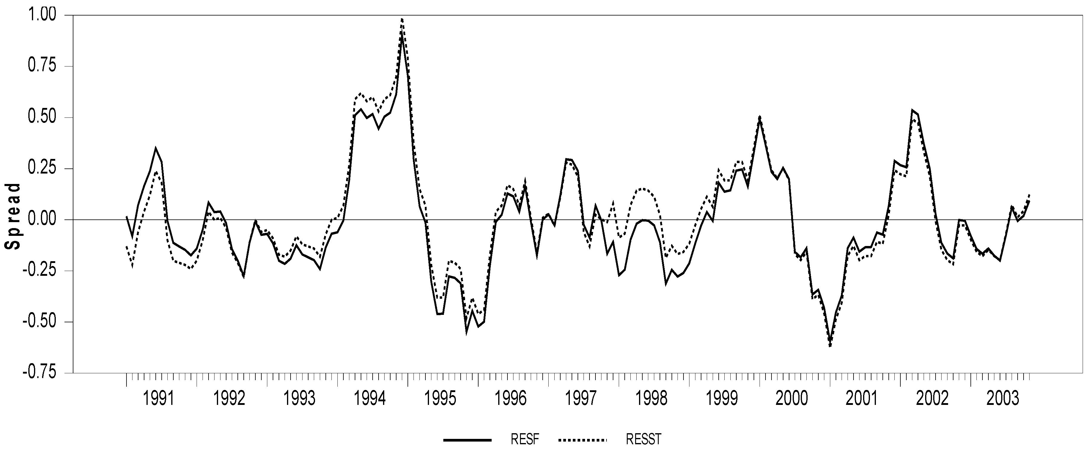
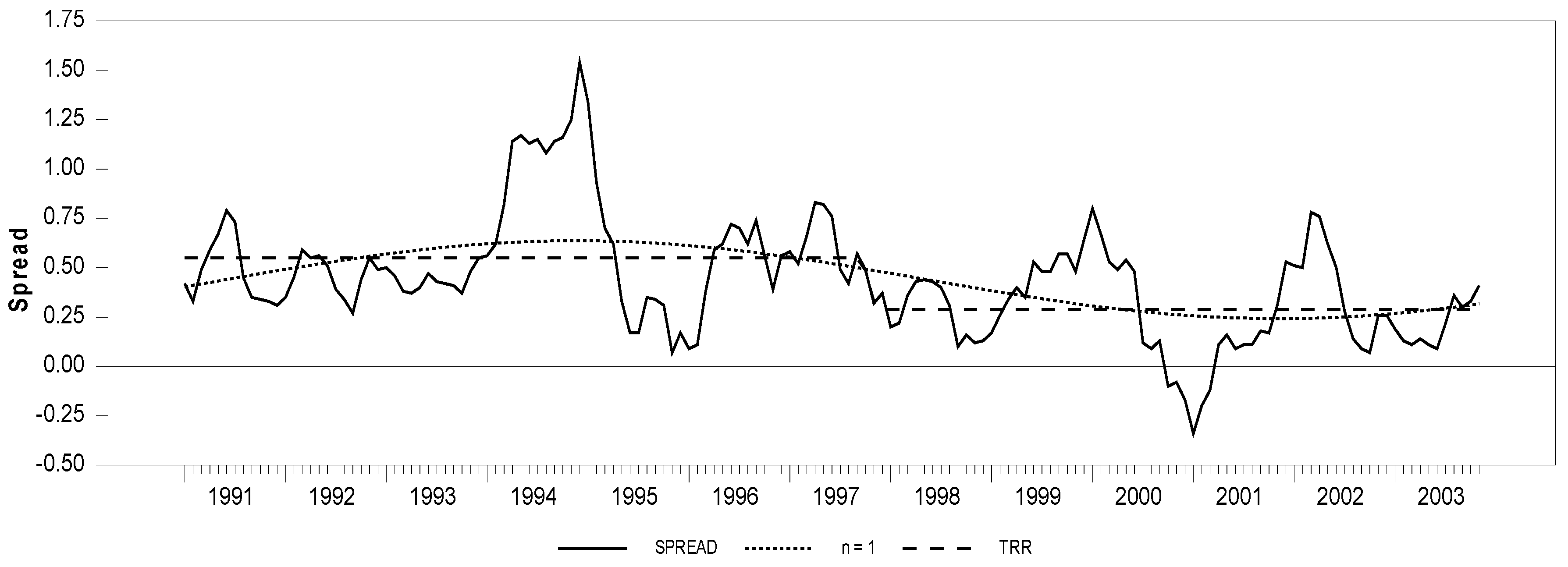
We observe from Figure 2 and Figure 3 that both methods exhibit similar de-trending patterns. We also find that the break parameter is located in the middle of the series and the pattern of structural break is very smooth. From the power simulation studies in the previous section, we know that the power of the LNV test improves if the location parameter is located in the middle of the sample. Furthermore, the smoothness of the transition enhances the power of the EL test. Therefore, EL and LNV tests are able to reject the unit root null convincingly.
Next, we apply the tests to the real exchange rate data. Christopoulos and Leon-Ledesma [9] attempt to model the structural breaks by means of the Fourier function because it allows for infrequent smooth temporary changes in the mean of the real exchange rate (RER) series and thereby is compatible with the long-run purchasing power parity (PPP). They have also claimed that they solve the PPP puzzle when there is a temporary structural break in the mean of the real RER series. The RER series obtained from Turkish data cover the period 1990:1–2003:11, see also Çorakcı et.al. [36] for more details.
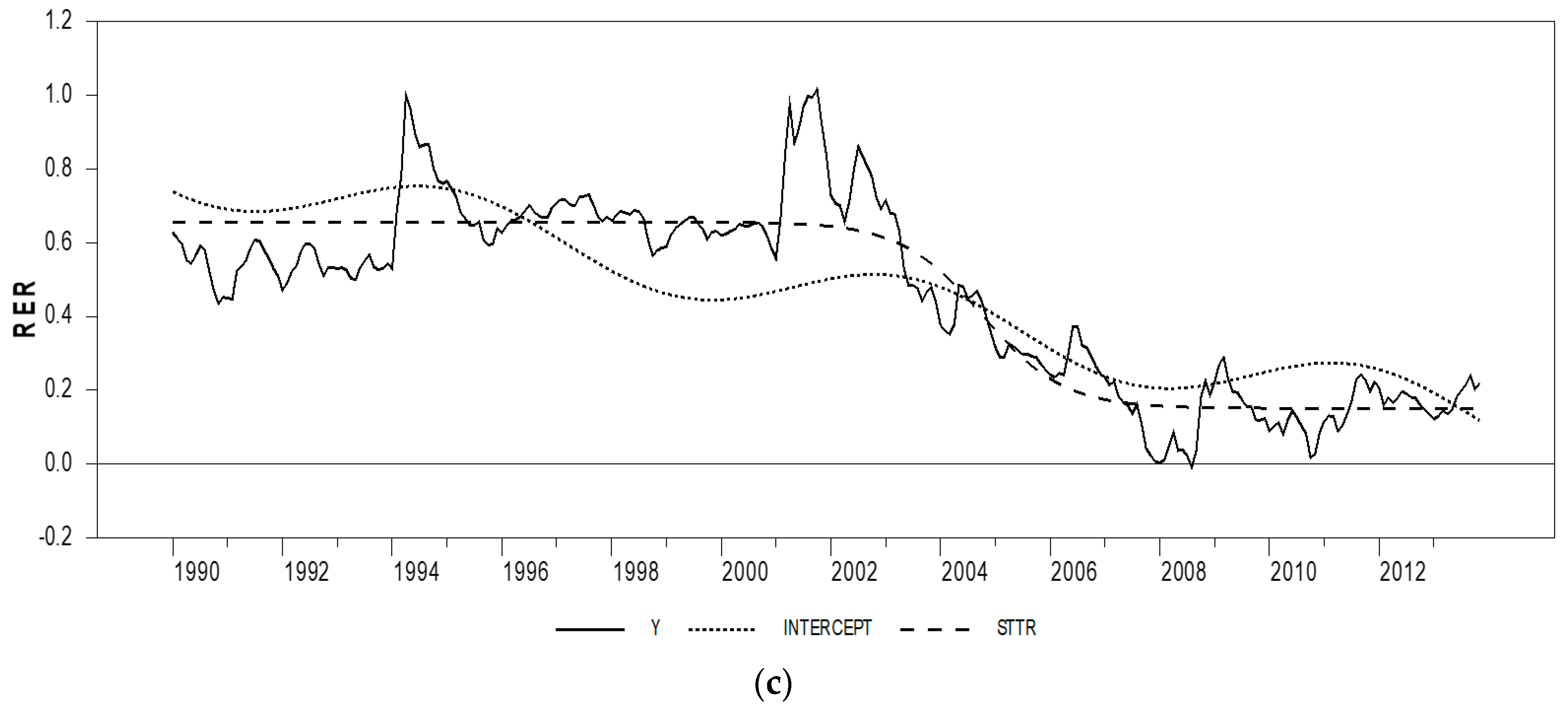
We plot the Turkey/US RER series in Figure 4, which provides a clear contradiction to the argument made by [9]. This is mainly due to the presence of sharp permanent breaks in the middle of the sample. As highlighted in the above power simulation studies, we find that the Fourier transform with low frequency fails to capture sharp breaks.
The OY test, which includes a STR de-trending, is the only test which can reject the null hypothesis of a unit root in the Turkish RER series. From the LNV, KSS and OY test results in Table 8, we may conclude that the Turkish RER series have two sources of non-linearity, namely structural break and state-dependent non-linearity. LNV and KSS tests do not reject the null hypothesis of unit root, but the OY test embedded both of them in its testing procedure, hence the only possibility of rejecting the null hypothesis by OY test is to have the two sources of nonlinearities in the RER series.
The two empirical applications suggest that it may be misleading to rely upon the result obtained from one particular test only. Therefore, we should perform several types of unit root test including the ones allowing for different types of structural breaks (e.g., smooth or sharp), non-linearity (e.g., STR or TAR) and both, when testing the stochastic property of a series. For instance, in the second example, we exactly determine that the RER series of Turkey includes both sharp structural break and state-dependent non-linearity. This result is obtained by employing several different tests. Hence, we can confidently eliminate the alternative structures for the RER series, for example smooth structural break with EL test, TAR type of non-linearity with EG and Sollis [15] test, and sharp break only by LNV test.

5. Conclusions

In this study, the de-trending strategies of structural break in unit root testing are compared. For comparative purposes two flexible methodologies, namely Fourier transforms and smooth transition regression, are used. Both of these methodologies are shown to be superior to each other in specific cases. These cases are listed at the end of Section 3. For example, if we have a series with sharp break in the middle of the sample, we have to use an ST type of de-trending in order to obtain power gains in determining the stochastic properties of the series in consideration. Using a structural break unit root test that employs the Fourier transforms for detecting structural breaks, erroneously leads to accepting the null hypothesis due to the over-filtration problem of the Fourier function. We can conclude that for each category of structural break that we classify in this study, the relevant de-trending strategy should be followed. As we also point out in the empirical part, all the relevant unit root tests must be carried out in order to identify the true structure of the DGP.

Author Contributions

Conceptualization, F.E. and T.O.; methodology, F.E.; software, F.E.; validation, F.E. and T.O.; formal analysis, F.E.; investigation, T.O.; data curation, F.E.; writing—original draft, F.E., T.O. and S.J.H.S.; writing—review and editing, S.M.N.; visualization, S.J.H.S. and S.M.N.; supervision, T.O.; funding acquisition, S.M.N. All authors have read and agreed to the published version of the manuscript.

Funding

The APC was funded by RHB Islamic Endowed Scholar in Finance research grant (vote: 53276). The authors are grateful to RHB Islamic Bank Berhad for the financial support.

Institutional Review Board Statement

Not applicable.

Informed Consent Statement

Not applicable.

Data Availability Statement

Publicly available datasets were analysed in this study. The data can be found here: http://www.time-series.net/time-series_papers, accessed on 1 January 2021.

Acknowledgments

A preliminary draft of this paper was presented at the 4th International Conference on Banking and Finance Perspectives, 2–3 May 2019, Famagusta, North Cyprus. We thank the conference participants for their comments and suggestions.

Conflicts of Interest

The authors declare no conflict of interest. The funders had no role in the design of the study; in the collection, analyses, or interpretation of data; in the writing of the manuscript, or in the decision to publish the results.

Appendix A

This appendix provides details about FADF and FKSS tests. Specifically, the critical values demeaned and detrended are provided for both tests. The asymptotic distribution of the tests is not available in the original paper; hence we also provide asymptotic distribution of both demeaned and detrended examples.
Proof of Proposition 1.
Suppose that Δ x t = u t under the null hypothesis. Thus, the proofs of (i) and (ii) are standard, see Hamilton [37] (p. 486). We can obtain the proofs of (iii) and (iv) from the continuous mapping theorem.
T 3 / 2 t = 1 T s i n ( 2 π k t T ) x t σ 0 1 s i n ( 2 π k r ) W ( r ) d r = σ f 3
T 3 / 2 t = 1 T c o s ( 2 π k t T ) x t σ 0 1 c o s ( 2 π k r ) W ( r ) d r = σ f 4
The other proofs related to asymptotic theory others are as follows:
T 1 t = 1 T sin ( 2 π k t T ) 0 1 sin ( 2 π k r ) d r = 1 2 π k [ 1 cos ( 2 π k ) ] = 0 T 1 t = 1 T cos ( 2 π k t T ) 0 1 cos ( 2 π k r ) d r = sin ( 2 π k ) 2 π k = 0 T 2 t = 1 T t sin ( 2 π k t T ) 0 1 r sin ( 2 π k r ) d r = sin ( 2 π k ) ( 2 π k ) 2 cos ( 2 π k ) 2 π k = 1 2 π k T 2 t = 1 T t cos ( 2 π k t T ) 0 1 r cos ( 2 π k r ) d r = cos ( 2 π k ) 1 ( 2 π k ) 2 + sin ( 2 π k ) 2 π k = 0 T 1 t = 1 T sin 2 ( 2 π k t T ) 0 1 sin 2 ( 2 π k r ) d r = 1 2 0 1 [ 1 cos ( 4 π k r ) ] d r = 1 2 [ 1 sin ( 4 π k ) 4 π k ] = 0.5 T 1 t = 1 T cos 2 ( 2 π k t T ) 0 1 cos 2 ( 2 π k r ) d r = 1 2 0 1 [ 1 + cos ( 4 π k r ) ] d r = 1 2 [ 1 + sin ( 4 π k ) 4 π k ] = 0.5 T 1 t = 1 T sin ( 2 π k t T ) cos ( 2 π k t T ) 0 1 sin ( 2 π k r ) cos ( 2 π k r ) d r = 1 2 0 1 sin ( 4 π k r ) d r = 1 8 π k [ 1 cos ( 4 π k ) ] = 0
Proof of Theorem 1.
We first examine demeaned case with α 1 = 0 in Equation (1). y t μ denote the OLS residuals from Equation (1) in the text with w t = ( 1 , s i n ( 2 π k t / T ) , c o s ( 2 π k t / T ) ) .
y t μ = x t w t ( θ ^ θ )
where θ = ( α 0 , φ 1 , φ 2 ) , θ ^ is the OLS estimator of θ and Δ x t = u t under the null hypothesis. We let w = ( w 1 , , w T ) , x = ( x 1 , , x T ) and Y T = d i a g ( T , T , T ) to have
Y T ( θ ^ θ ) = [ Y T 1 w w Y T 1 ] 1 Y T 1 w x
From Equations (A1) and (A2), we can show that
T 1 / 2 y [ T r ] μ = T 1 / 2 x [ T r ] T 1 / 2 w [ T r ] ( θ ^ θ ) T 1 / 2 y [ T r ] μ = T 1 / 2 x [ T r ] T 1 / 2 w [ T r ] Y T 1 [ Y T 1 w w Y T 1 ] 1 Y T 1 w x T 1 / 2 y [ T r ] μ = T 1 / 2 x [ T r ] T 1 w [ T r ] [ Y T 1 w w Y T 1 ] 1 Y T 1 w x
According to functional central limit theorems, the first term in (A3) is follows:
T 1 / 2 x [ T r ] = T 1 / 2 t = 1 [ T r ] u t σ W ( r )
Then, the second term in (A.3) follows:
[ Y T 1 w w Y T 1 ] 1 = [ 1 T 1 t = 1 T s i n ( 2 π k t T ) T 1 t = 1 T c o s ( 2 π k t T ) T 1 t = 1 T s i n 2 ( 2 π k t T ) T 1 t = 1 T s i n ( 2 π k t T ) c o s ( 2 π k t T ) T 1 t = 1 T c o s 2 ( 2 π k t T ) ] 1 [ 1 0 0 1 / 2 0 1 / 2 ] 1 = [ 1 0 0 2 0 2 ]
T 1 Y T 1 w x = [ T 1 / 2 t = 1 T x t T 1 / 2 t = 1 T s i n ( 2 π k t T ) x t T 1 / 2 t = 1 T c o s ( 2 π k t T ) x t ] [ σ f 1 σ f 3 σ f 4 ]
Then, we can write that:
T 1 w [ T r ] [ Y T 1 w w Y T 1 ] 1 Y T 1 w x [ 1 s i n ( 2 π k r ) c o s ( 2 π k r ) ] [ 1 0 0 0 2 0 0 0 2 ] [ σ f 1 σ f 3 σ f 4 ]
Therefore, we can obtain demeaned Brownian motion by combining the results in Equations (A4) and (A7):
1 σ T y [ T r ] μ W μ ( k , r ) = W ( r ) f 1 2 s i n ( 2 π k r ) f 3 2 c o s ( 2 π k r ) f 4
Secondly, we examine the detrended case with α 1 0 in Equation (1). y t τ denote the OLS residuals from Equation (1) in the text with w t = ( 1 , s i n ( 2 π k t / T ) , c o s ( 2 π k t / T ) ) .
y t τ = x t w t ( θ ^ θ )
where θ = ( α 0 , α 1 , φ 1 , φ 2 ) , θ ^ is the OLS estimator of θ and Δ x t = u t under the null hypothesis. Let Y T = d i a g ( T , T 3 / 2 , T , T ) in (A2). Using Equations (A9) and (A2), we can write:
T 1 / 2 y [ T r ] τ = T 1 / 2 x [ T r ] T 1 w [ T r ] [ Y T 1 w w Y T 1 ] 1 Y T 1 w x
The second term in (A.10) follows:
[ Y T 1 w w Y T 1 ] 1 = [ 1 T 2 t = 1 T t T 1 t = 1 T s i n ( 2 π k t T ) T 1 t = 1 T c o s ( 2 π k t T ) T 3 t = 1 T t 2 T 2 t = 1 T t s i n ( 2 π k t T ) T 2 t = 1 T t c o s ( 2 π k t T ) T 1 t = 1 T s i n 2 ( 2 π k t T ) T 1 t = 1 T s i n ( 2 π k t T ) c o s ( 2 π k t T ) T 1 t = 1 T c o s 2 ( 2 π k t T ) ] 1 [ 1 1 / 2 0 0 1 / 2 1 / 3 1 / ( 2 π k ) 0 0 1 / ( 2 π k ) 1 / 2 0 0 1 / 2 0 1 / 2 ] 1 = [ b 11 b 12 b 13 b 14 b 21 b 22 b 23 b 24 b 31 b 32 b 33 b 34 b 41 b 42 b 43 b 44 ]
where b 11 = ( 4 n 2 6 ) / ( n 2 6 ) , b 12 = b 21 = 6 n 2 / ( n 2 6 ) , b 13 = b 31 = 6 n / ( n 2 6 ) , b 14 = b 41 = 0 , b 22 = 12 n 2 / ( n 2 6 ) , b 23 = b 32 = 12 n / ( n 2 6 ) , b 24 = b 42 = 0 , b 33 = 2 n 2 / ( n 2 6 ) , b 34 = b 43 = 0 , b 44 = 2 and n = π k .
T 1 Y T 1 w x = [ T 1 / 2 t = 1 T x t T 3 / 2 t = 1 T t x t T 1 / 2 t = 1 T s i n ( 2 π k t T ) x t T 1 / 2 t = 1 T c o s ( 2 π k t T ) x t ] [ σ f 1 σ f 2 σ f 3 σ f 4 ]
Then, we can write that:
T 1 w [ T r ] [ Y T 1 w w Y T 1 ] 1 Y T 1 w x = [ 1 r s i n ( 2 π k r ) c o s ( 2 π k r ) ] [ b 11 b 12 b 13 0 b 21 b 22 b 23 0 b 31 b 32 b 33 0 0 0 0 b 44 ] [ σ f 1 σ f 2 σ f 3 σ f 4 ]
Therefore, we can obtain detrended Brownian motion by combining the results in Equations (A4) and (A13).
1 σ T y [ T r ] τ W τ ( k , r ) = W ( r ) ( b 11 f 1 + b 12 f 2 + b 13 f 3 ) ( b 21 f 1 + b 22 f 2 + b 23 f 3 ) r ( b 31 f 1 + b 32 f 2 + b 33 f 3 ) s i n ( 2 π k r ) b 44 f 4 c o s ( 2 π k r )
Hence, using above results, under the null we can obtain that:
t i F A D F d 0 1 W i ( k , r ) d W ( r ) ( 0 1 W i ( k , r ) 2 d r ) 1 / 2                     i = μ , τ
t i F K S S d 0 1 W i ( k , r ) 3 d W ( r ) ( 0 1 W i ( k , r ) 6 d r ) 1 / 2                     i = μ , τ

References

  1. Enders, W.; Lee, J. A unit root test using a Fourier series to approximate smooth breaks. Oxf. Bull. Econ. Stat. 2012, 74, 574–599. [Google Scholar] [CrossRef] [Green Version]
  2. Enders, W.; Lee, J. The flexible Fourier form and Dickey–Fuller type unit root tests. Econ. Lett. 2012, 117, 196–199. [Google Scholar] [CrossRef]
  3. Bai, J.; Perron, P. Estimating and testing linear models with multiple structural changes. Econometrica 1998, 66, 47–78. [Google Scholar] [CrossRef]
  4. Kejrival, M.; Lopez, C. Unit roots, level shifts and trend breaks in per capita output: A robust evaluation. Econom. Rev. 2013, 32, 892–927. [Google Scholar] [CrossRef] [Green Version]
  5. Gallant, A.R. On the bias in flexible functional forms and an essentially unbiased form: The Fourier flexible form. J. Econom. 1981, 15, 211–245. [Google Scholar] [CrossRef]
  6. Leybourne, S.; Newbold, P.; Vougas, D. Unit roots and smooth transitions. J. Time Ser. Anal. 1998, 19, 83–97. [Google Scholar] [CrossRef]
  7. Rodrigues, P.; Taylor, A.M.R. The flexible Fourier form and local generalized least squares de-trended unit root tests. Oxf. Bull. Econ. Stat. 2012, 74, 736–759. [Google Scholar] [CrossRef]
  8. Omay, T.; Emirmahmutoglu, F. The comparison of power and optimization algorithms on unit root testing with smooth transition. Comput. Econ. 2017, 49, 623–651. [Google Scholar] [CrossRef]
  9. Christopoulos, D.K.; Leon-Ledesma, M.A. Smooth breaks and non-linear mean reversion: Post-Bretton Woods real exchange rates. J. Int. Money Financ. 2010, 29, 1076–1093. [Google Scholar] [CrossRef] [Green Version]
  10. Omay, T.; Yildirim, Y. Nonlinearity and smooth breaks in unit root testing. Econom. Lett. 2014, 1, 2–9. [Google Scholar]
  11. Kapetanios, G.; Shin, Y.; Snell, A. Testing for a unit root in the nonlinear STAR framework. J. Econom. 2003, 112, 359–379. [Google Scholar] [CrossRef]
  12. Becker, R.; Enders, W.; Hurn, S. A general test for time dependence in parameters. J. Appl. Econom. 2004, 19, 899–906. [Google Scholar] [CrossRef] [Green Version]
  13. Becker, R.; Enders, W.; Lee, J. A stationarity test in the presence of an unknown number of smooth breaks. J. Time Ser. Anal. 2006, 27, 38–409. [Google Scholar] [CrossRef]
  14. Luukkonen, R.; Saikkonen, P.; Teräsvirta, T. Testing linearity against smooth transition autoregressive models. Biometrika 1988, 75, 491–499. [Google Scholar] [CrossRef]
  15. Sollis, R. Asymmetric adjustment and smooth transitions: A combination of some unit root tests. J. Time Ser. Anal. 2004, 25, 409–417. [Google Scholar] [CrossRef]
  16. Dickey, D.A.; Fuller, W.A. Distribution of the estimators for autoregressive time series with a unit root. J. Am. Stat. Assoc. 1979, 74, 427–431. [Google Scholar]
  17. Pinsky, M.A. Introduction to Fourier Analysis and Wavelets; American Mathematical Society: Pacific Grove, CA, USA, 2009. [Google Scholar]
  18. Davies, R.B. Hypothesis testing when a nuisance parameter is only identified under the alternative. Biometrika 1987, 47, 33–43. [Google Scholar]
  19. Gallant, A.R.; Souza, G. On the asymptotic normality of Fourier flexible form estimates. J. Econom. 1991, 50, 329–353. [Google Scholar] [CrossRef] [Green Version]
  20. Bierens, H.J. Testing the unit root with drift hypothesis against nonlinear trend stationarity with an application to the US price level and interest rate. J. Econom. 1997, 81, 29–64. [Google Scholar] [CrossRef]
  21. Cai, Y.; Omay, T. Using double frequency in Fourier Dickey–Fuller unit root test. Comput. Econ. 2021, 1–26. [Google Scholar]
  22. Omay, T.; Çorakci, A.; Emirmahmutoglu, F. Real interest rates: Nonlinearity and structural breaks. Empir. Econ. 2017, 52, 283–307. [Google Scholar] [CrossRef]
  23. Omay, T.; Hasanov, M.; Shin, Y. Testing for unit roots in dynamic panels with smooth breaks and cross-sectionally dependent errors. Comput. Econ. 2018, 52, 167–193. [Google Scholar] [CrossRef]
  24. Omay, T.; Emirmahmutoglu, F.; Hasanov, M. Structural break, nonlinearity and asymmetry: A re-examination of PPP proposition. Appl. Econ. 2018, 50, 1289–1308. [Google Scholar] [CrossRef] [Green Version]
  25. Omay, T.; Shahbaz, M.; Hasanov, M. Testing PPP hypothesis under temporary structural breaks and asymmetric dynamic adjustments. Appl. Econ. 2020, 52, 3479–3497. [Google Scholar] [CrossRef]
  26. Omay, T.; Emirmahmutoglu, F.; Shahzad, S.J.H. Comparison of optimization algorithms for selecting the fractional frequency in Fourier form unit root tests. Appl. Econ. 2021, 53, 761–780. [Google Scholar] [CrossRef]
  27. Shahbaz, M.; Omay, T.; Roubaud, D. Sharp and smooth breaks in unit root testing of renewable energy consumption. J. Energy Dev. 2018, 44, 5–40. [Google Scholar]
  28. Türkvatan, A.; Hayfavi, A.; Omay, T. A regime switching model for temperature modeling and applications to weather derivatives pricing. Math. Financ. Econ. 2020, 14, 1–42. [Google Scholar] [CrossRef]
  29. Aktan, C.; Iren, P.; Omay, T. Market development and market efficiency: Evidence based on nonlinear panel unit root tests. Eur. J. Financ. 2019, 25, 979–993. [Google Scholar] [CrossRef]
  30. Canarella, G.; Gupta, R.; Miller, S.M.; Omay, T. Does UK’s real GDP have a unit root? Evidence from a multi-century perspective. Appl. Econ. 2020, 52, 1070–1087. [Google Scholar] [CrossRef]
  31. Emirmahmutoglu, F.; Gupta, R.; Miller, S.M.; Omay, T. Is real per capita state personal income stationary? New nonlinear, asymmetric panel-data evidence. Bull. Econ. Res. 2020, 72, 50–62. [Google Scholar] [CrossRef]
  32. Hasdemir, E.; Tolga, O.; Zulal, D. Testing the current account sustainability for BRICS countries: Evidence from a nonlinear framework. Econ. Bull. 2019, 39, 310–320. [Google Scholar]
  33. Omay, T.; Ozcan, B.; Shahbaz, M. Testing the hysteresis effect in the US state-level unemployment series. J. Appl. Econ. 2020, 23, 329–348. [Google Scholar] [CrossRef]
  34. Omay, T. Fractional frequency flexible Fourier form to approximate smooth breaks in unit root testing. Econ. Lett. 2015, 134, 123–126. [Google Scholar] [CrossRef]
  35. Enders, W.; Granger, C.W.J. Unit root tests and asymmetric adjustment with an example using the term structure of interest rates. J. Bus. Econ. Stat. 1998, 16, 304–311. [Google Scholar]
  36. Çorakcı, A.; Emirmahmutoglu, F.; Omay, T. ESTR type smooth break unit root test. Econ. Bull. 2017, 37, 1541–1548. [Google Scholar]
  37. Hamilton, J.D. Time Series Analysis; Princeton University Press: Princeton, NJ, USA, 1994. [Google Scholar]
Figure 1. Non–linearity around smooth break and the behaviour of low frequency Fourier transforms.
Mathematics 09 00371 g001
Figure 2. The R1–T–bill spread, the Fourier intercept and the smooth transition (ST) trend.
Mathematics 09 00371 g002
Figure 3. Residual from de–trending with Fourier intercept and the ST trend.
Mathematics 09 00371 g003
Figure 4. Plots of the Turkey/US real exchange rate (RER) series. (a) The Fourier intercept k = 1 and the ST trend–Model A; (b) residuals from de-trending with Fourier intercept k = 1 and the ST trend–Model A; (c) the Fourier intercept k = 1 and the ST trend–Model A.
Mathematics 09 00371 g004aMathematics 09 00371 g004b
Table 1. Asymptotic critical values of FADF and FKSS test statistics.
t μ F A D F t μ F K S S
k 1%5%10%1%5%10%
1−4.309−3.745−3.448−4.158−3.574−3.273
2−3.886−3.243−2.905−3.807−3.246−2.951
3−3.693−3.056−2.727−3.664−3.094−2.807
4−3.582−2.974−2.652−3.613−3.037−2.755
5−3.578−2.933−2.626−3.572−3.020−2.734
t τ F A D F t τ F K S S
k 1%5%10%1%5%10%
1−4.777−4.255−3.982−4.625−4.089−3.810
2−4.532−3.960−3.657−4.352−3.798−3.497
3−4.339−3.732−3.411−4.203−3.622−3.322
4−4.205−3.610−3.298−4.111−3.539−3.254
5−4.130−3.536−3.237−4.071−3.503−3.216
Table 2. The simulated powers of alternative tests under the FKSS-DGP.
φ 1 φ 2 θ γ t μ F K S S s α N L t μ F A D F s α t s α F α t N L , τ τ τ
0.05.00.01−0.10.0450.0070.0800.0100.0140.0090.0090.007
3.00.00.01−0.10.0560.0280.0740.0360.0420.0320.0460.047
3.05.00.01−0.10.0330.0040.0730.0030.0050.0020.0030.002
0.05.00.01−1.00.0910.0010.1950.0040.0080.0030.0050.001
3.00.00.01−1.00.1520.0940.1930.0690.0770.0730.1070.080
3.05.00.01−1.00.0780.0010.1960.0010.0010.0010.0010.001
0.05.00.01−1.50.1230.0010.2700.0010.0020.0010.0070.001
3.00.00.01−1.50.2060.1450.2700.1000.1010.0950.1440.114
3.05.00.01−1.50.1100.0010.2650.0010.0010.0010.0010.001
0.05.01.0−0.10.0780.0010.1570.0020.0040.0010.0010.002
3.00.01.0−0.10.0940.0640.1610.0570.0690.0550.0640.066
3.05.01.0−0.10.0770.0010.1600.0010.0010.0010.0010.001
0.05.01.0−1.00.9930.0121.0000.0010.0010.0010.1940.001
3.00.01.0−1.00.9980.9301.0000.9990.9950.9980.9470.963
3.05.01.0−1.00.9860.0011.0000.0010.0010.0010.0020.001
0.05.01.0−1.51.0000.1671.0000.0040.0370.0060.7300.004
3.00.01.0−1.51.0001.0001.0001.0001.0001.0001.0001.000
3.05.01.0−1.51.0000.0101.0000.0030.0750.0090.1300.001
Note: t μ F K S S , s α N L , t μ F A D F , s α , t s α , F α , t N L , τ and τ τ indicate the FKSS test with intercept only, the Omay and Yıldırım [10] test for Model A, the FADF test with intercept only, the Leybourne et al. [6] test for Model A, the Sollis [15] t and F tests for Model A, the Kapetanios et al. [11] test with intercept and trend, and the Dickey–Fuller [16] tests with intercept and trend, respectively.
Table 3. The over filtration of the Fourier transforms under the FKSS-DGP.
k φ 1 φ 2 θ γ T = 100
1.00.05.00.01−0.10.090
1.03.00.00.01−0.10.098
1.03.05.00.01−0.10.088
1.00.05.00.01−1.00.158
1.03.00.00.01−1.00.175
1.03.05.00.01−1.00.148
1.00.05.00.1−0.10.078
1.03.00.00.1−0.10.086
1.03.05.00.1−0.10.071
Note: In this simulation study, 2000 draws are used.
Table 4. The simulated powers of alternative tests under the KSS 1st DGP.
φ 1 φ 2 θ γ t μ F K S S s α N L t μ F A D F s α t s α F α t N L , τ τ τ
0.00.00.01−0.10.0830.0440.0800.0410.0470.0400.0660.070
0.00.00.01−0.50.2160.0840.1330.0680.0680.0650.1360.135
0.00.00.01−1.00.3930.1380.1930.1040.1010.0980.2660.201
0.00.00.01−1.50.5660.2270.2650.1650.1500.1580.4350.334
0.00.00.05−0.10.1210.0640.0990.0510.0410.0460.1030.098
0.00.00.05−0.50.6340.2790.3440.1850.1630.1790.5410.447
0.00.00.05−1.00.9440.7430.7650.5260.4730.5110.9000.911
0.00.00.05−1.50.9940.9150.9660.8600.7510.8500.9830.993
0.00.00.1−0.10.1400.0590.1180.0550.0550.0510.1110.116
0.00.00.1−0.50.8300.5030.6170.3700.3260.3630.7650.803
0.00.00.1−1.00.9950.9400.9880.9320.8470.9250.9910.995
0.00.00.1−1.51.0000.9981.0001.0000.9890.9991.0001.000
0.00.00.5−0.10.1340.0810.1530.0750.0650.0670.1320.175
0.00.00.5−0.50.9510.8730.9960.9670.8950.9580.9631.000
0.00.00.5−1.01.0001.0001.0001.0001.0001.0001.0001.000
0.00.00.5−1.51.0001.0001.0001.0001.0001.0001.0001.000
0.00.01.0−0.10.1270.0700.1580.0710.0630.0660.1360.188
0.00.01.0−0.50.9440.8940.9990.9920.9690.9870.9691.000
0.00.01.0−1.01.0001.0001.0001.0001.0001.0001.0001.000
0.00.01.0−1.51.0001.0001.0001.0001.0001.0001.0001.000
Note: See Table 2 note.
Table 5. The simulated powers of alternative tests under the Leybourne, Newbold and Vougas (LNV)-DGP.
α 2 λ τ t μ F K S S s α N L t μ F A D F s α t s α F α t N L , τ τ τ
2.00.010.20.3490.2910.6340.4050.3490.3920.4710.749
2.00.10.20.3390.2440.5470.3730.2970.3580.4060.682
2.00.20.20.3330.2490.4920.3300.2630.3150.3880.640
2.00.50.20.3100.2450.4330.3130.2750.3010.3600.603
2.00.70.20.3100.2290.4280.2940.2510.2790.3650.605
2.01.00.20.3030.2230.4220.2930.2430.2840.3850.588
2.02.50.20.2940.2390.4110.3070.2430.2920.3530.587
2.05.00.20.2990.2010.4200.2810.2370.2680.3540.577
2.010.00.20.2970.2340.4170.2890.2500.2830.3570.598
2.00.010.50.3310.2860.6150.4010.3440.3800.4500.735
2.00.10.50.2690.2480.5200.3680.3020.3580.3890.663
2.00.20.50.2650.2530.5300.3630.2930.3500.3710.617
2.00.50.50.2590.2380.5150.3760.3050.3620.3640.619
2.00.70.50.2490.2490.5090.3450.2660.3210.3440.592
2.01.00.50.2500.2450.5080.3550.2730.3390.3310.577
2.02.50.50.2470.2330.5060.3470.2670.3320.3270.580
2.05.00.50.2460.2440.4990.3450.2730.3290.3360.589
2.010.00.50.2470.2430.4990.3660.2780.3430.3260.608
5.00.010.20.5160.5860.7930.6060.6330.6140.6800.867
5.00.10.20.3850.3500.4070.4360.3930.4290.4140.600
5.00.20.20.1700.2230.3490.3160.2630.3000.2820.371
5.00.50.20.2950.1650.0980.2400.1960.2260.2010.210
5.00.70.20.2830.1780.0850.2520.2130.2390.2010.186
5.01.00.20.2760.1750.0750.2500.2080.2410.1840.174
5.02.50.20.2600.1930.0700.2420.1880.2370.1970.163
5.05.00.20.2580.2040.0730.2530.2010.2390.1950.177
5.010.00.20.2580.1980.0750.2540.2120.2420.2000.183
5.00.010.50.4790.4930.7550.5490.5290.5550.6230.839
5.00.10.50.1710.2980.3300.4400.3670.4240.3410.596
5.00.20.50.1710.2700.3500.4260.3400.4070.2620.389
5.00.50.50.1740.2670.2880.3980.3120.3790.1750.241
5.00.70.50.1680.2520.2640.3750.2830.3540.1710.218
5.01.00.50.1600.2290.2450.3490.2670.3300.1430.191
5.02.50.50.1530.2580.2360.3320.2580.3120.1500.189
5.05.00.50.1580.2710.2440.3500.2760.3350.1700.211
5.010.00.50.1560.2670.2430.3600.2720.3430.1760.193
10.00.010.20.6760.9670.9580.9140.9600.9300.9620.981
10.00.10.20.3440.4780.1730.5480.5490.5400.4890.365
10.00.20.20.2370.2690.0120.3690.3050.3570.1340.041
10.00.50.20.1670.2200.0000.3120.2400.2950.0320.002
10.00.70.20.1530.2050.0000.3150.2530.3070.0290.003
10.01.00.20.1400.2200.0000.2890.2300.2730.0210.001
10.02.50.20.0990.2300.0000.2990.2390.2820.0390.001
10.05.00.20.0890.2500.0000.2980.2420.2930.0560.001
10.010.00.20.0870.2700.0000.3090.2560.2950.0760.002
10.00.010.50.6290.9070.9150.8440.9010.8680.9130.958
10.00.10.50.0510.3300.0640.4610.3670.4490.2240.328
10.00.20.50.0930.2980.0810.4300.3450.4150.0820.054
10.00.50.50.1440.2590.0340.3920.3110.3820.0190.003
10.00.70.50.1550.2350.0240.3670.2870.3530.0130.002
10.01.00.50.1570.2530.0160.3450.2730.3270.0050.002
10.02.50.50.1350.2490.0150.3260.2560.3040.0160.002
10.05.00.50.1320.2820.0180.3530.2760.3370.0530.002
10.010.00.50.1290.2770.0180.3380.2690.3260.0620.002
Note: See Table 2 note.
Table 6. The power comparison of alternative tests: Omay and Yıldırım data-generating processes (OY-DGP).
α 2 λ τ θ γ t μ F K S S s α N L t μ F A D F s α t s α F α t N L , τ τ τ
2.00.50.20.01−0.10.0780.0620.0850.0460.0460.0340.0510.039
2.00.50.21.0−0.10.1130.0860.1640.0760.0700.0680.0570.061
2.00.50.20.01−1.00.1670.1640.1960.1300.1480.1160.2290.210
2.00.50.21.0−1.01.0001.0001.0001.0001.0001.0001.0001.000
2.00.50.50.01−0.10.0760.0700.0910.0640.0640.0520.0520.039
2.00.50.51.0−0.10.1100.1000.1800.0920.0840.0860.0550.057
2.00.50.50.01−1.00.1760.1520.2130.1320.1100.1080.2180.216
2.00.50.51.0−1.00.9971.0001.0001.0001.0001.0001.0001.001
2.05.00.20.01−0.10.0720.0500.0800.0380.0420.0260.0510.047
2.05.00.21.0−0.10.1040.1160.1510.1100.0920.0980.0670.069
2.05.00.20.01−1.00.1590.1600.1910.1300.1260.1240.2400.211
2.05.00.21.0−1.01.0001.0001.0001.0001.0001.0001.0011.001
2.05.00.50.01−0.10.0770.0520.0880.0420.0400.0320.0500.043
2.05.00.51.0−0.10.1060.0960.1750.1180.0880.0980.0550.063
2.05.00.50.01−1.00.1750.1900.2130.1620.1300.1500.2030.189
2.05.00.51.0−1.00.9971.0001.0001.0001.0001.0001.0011.001
5.00.50.20.01−0.10.0570.0460.0530.0450.0530.0440.0460.036
5.00.50.21.0−0.10.1060.0850.0680.0750.0740.0710.0500.039
5.00.50.20.01−1.00.1360.1210.0820.0890.0990.0910.1650.117
5.00.50.21.0−1.01.0000.9960.8760.9980.9960.9970.9490.980
5.00.50.50.01−0.10.0660.0860.0770.0380.0420.0380.0390.036
5.00.50.51.0−0.10.0870.1400.1260.0800.0740.0790.0320.029
5.00.50.50.01−1.00.1150.1710.1540.1180.0960.1180.1110.121
5.00.50.51.0−1.00.9571.0000.9991.0001.0001.0000.9490.997
5.05.00.20.01−0.10.0470.0420.0420.0290.0390.0260.0400.034
5.05.00.21.0−0.10.0820.0770.0530.0550.0590.0570.0510.037
5.05.00.20.01−1.00.1160.1030.0680.0650.0730.0600.1600.106
5.05.00.21.0−1.01.0000.9940.7810.9980.9960.9960.9250.960
5.05.00.50.01−0.10.0590.0890.0690.0310.0370.0300.0250.023
5.05.00.51.0−0.10.0780.0990.1080.0860.0630.0810.0460.043
5.05.00.50.01−1.00.1070.1650.1350.0990.0870.0940.1020.097
5.05.00.51.0−1.00.9501.0000.9971.0001.0001.0000.8940.987
10.00.50.20.01−0.10.0500.0560.0070.0120.0160.0080.0300.015
10.00.50.21.0−0.10.0700.0760.0030.0680.0520.0540.0280.008
10.00.50.20.01−1.00.0930.1200.0030.0800.0600.0740.0450.017
10.00.50.21.0−1.00.9811.0000.0001.0001.0001.0000.3560.004
10.00.50.50.01−0.10.0810.0920.0370.0420.0400.0340.0130.007
10.00.50.51.0−0.10.0930.1140.0360.0880.0680.0720.0100.007
10.00.50.50.01−1.00.1120.2420.0410.1610.1910.1110.0250.017
10.00.50.51.0−1.00.7911.0000.3251.0001.0001.0000.3640.030
10.05.00.20.01−0.10.0280.1140.0040.0280.0340.0160.0430.012
10.05.00.21.0−0.10.0350.1440.0020.0740.0680.0680.0360.007
10.05.00.20.01−1.00.0500.1880.0010.0700.0860.0640.0300.009
10.05.00.21.0−1.00.9521.0000.0001.0001.0001.0000.3680.001
10.05.00.50.01−0.10.0600.1600.0210.0600.0960.0620.0210.006
10.05.00.51.0−0.10.0750.2740.0210.1480.1800.1440.0190.003
10.05.00.50.01−1.00.0940.3980.0240.1900.1980.1820.0360.017
10.05.00.51.0−1.00.7771.0000.1631.0001.0001.0000.2890.007
Note: See Table 2 note.
Table 7. Empirical application to the term structure data over 1990:1–2003:11.
t μ F A D F τ D F _ C C L t μ F K S S F t N L E L
−3.720 ***−3.707 ***−3.209−2.730
s α t s α F α s α N L
−4.789 **−2.0997.733−3.286
τ τ t N L , τ EG
−2.517−2.6093.499
Note 1: We use the same lag order, 12 for all the tests with both intercept and trend. **, and *** indicate 5% and 10% significance level, respectively. Note 2: t μ F A D F is the FADF test with intercept only, τ D F _ C C L is the critical values for FADF test generated by Christopoulos and Leon-Ledesma [9] methodology. t μ F K S S is the FKSS test with intercept only, F t N L E L FKSS test generated by Enders and Lee [1] methodology. s α Leybourne et al. [6] test for Model A (LNV), t s α and F α Sollis [15] t and F tests for Model A (S), s α N L Omay and Yıldırım [10] test for Model A (OY), τ τ Dickey and Fuller [16] test with intercept and trend (ADF), t N L , τ Kapetanios et al. [11] test with intercept and trend (KSS) and EG is the F test of Enders and Granger [21].
Table 8. Empirical application to the Turkey/US real exchange rate over 1990:1–2013:11.
t μ F A D F τ D F _ C C L t μ F K S S F t N L E L
−2.625−2.634−2.870−3.096
s α t s α F α s α N L
−1.186−1.9515.624−3.497 ***
τ μ t N L , τ EG
−1.124−2.7283.565
Note 1: We use the Akaike information criterion (AIC) for selecting the lag values. *** indicates 10% significance level. Note 2: See Table 7 Note 2.
Publisher’s Note: MDPI stays neutral with regard to jurisdictional claims in published maps and institutional affiliations.