A New Method of Measurement Matrix Optimization for Compressed Sensing Based on Alternating Minimization

Abstract

In this paper, a new method of measurement matrix optimization for compressed sensing based on alternating minimization is introduced. The optimal measurement matrix is formulated in terms of minimizing the Frobenius norm of the difference between the Gram matrix of sensing matrix and the target one. The method considers the simultaneous minimization of the mutual coherence indexes including maximum mutual coherence ${\mu }_{max}$, t-averaged mutual coherence ${\mu }_{ave}$ and global mutual coherence ${\mu }_{all}$, and solves the problem that minimizing a single index usually results in the deterioration of the others. Firstly, the threshold of the shrinkage function is raised to be higher than the Welch bound and the relaxed Equiangular Tight Frame obtained by applying the new function to the Gram matrix is taken as the initial target Gram matrix, which reduces ${\mu }_{ave}$ and solves the problem that ${\mu }_{max}$ would be larger caused by the lower threshold in the known shrinkage function. Then a new target Gram matrix is obtained by sequentially applying rank reduction and eigenvalue averaging to the initial one, leading to lower. The analytical solutions of measurement matrix are derived by SVD and an alternating scheme is adopted in the method. Simulation results show that the proposed method simultaneously reduces the above three indexes and outperforms the known algorithms in terms of reconstruction performance.

1. Introduction

Compressed sensing (CS) [1] can sample the sparse or compressible signals at a sub-Nyquist rate, which brings great convenience for data storage, transmission, and processing. By adopting the reconstruction algorithms, the signal can be exactly reconstructed from the sampled data. As a marvel way of signal processing, CS is applied in different fields such as image encryption [2], wideband spectrum sensing [3], wireless sensor network data processing [4], etc.

The original signal $\mathit{x}\in {\mathit{R}}^{N\times 1}$ is assumed to have a sparse representation in a known domain $\mathit{\Psi }\in {\mathit{R}}_N^{N\times L}$($N\le L$) as $x=\mathit{\Psi }\mathit{s}$ where $\mathit{\Psi }$ is the dictionary matrix and $s$ is a $K$-sparse signal. The incomplete measurement $\mathit{y}\in {\mathit{R}}^{M\times 1}$ is obtained through the linear model

$$\mathit{y}=\mathit{\Phi }\mathit{x}=\mathit{D}\mathit{s}$$

(1)

where $\mathit{\Phi }\in {\mathit{R}}^{M\times N}$($M<N$) is called the measurement matrix and $\mathit{D}=\mathit{\Phi }\mathit{\Psi }$ is the sensing matrix.

Some specific properties of $\mathit{\Phi }$ have great impacts on the reconstruction performance. In [5,6], spark and restricted isometric property (RIP) are respectively proposed as the sufficient conditions on $\mathit{\Phi }$ to recovery guarantee. However, computing the spark of a matrix has combinatorial complexity and certifying RIP for a matrix requires combinatorial search, that is to say, these tasks are NP-hard and difficult to accomplish. To a large extent, the coherence between $\mathit{\Phi }$ and $\mathit{\Psi }$ reflects the performance of meeting the above conditions. Actually, the coherence is equivalent to the mutual coherence of $\mathit{D}$. Since the mutual coherence can be easily manipulated to provide recovery guarantees, it is commonly used to measure the performance of $\mathit{\Phi }$. The frequently-used mutual coherence indexes include the maximum mutual coherence ${\mu }_{max}$ [7], t-averaged mutual coherence ${\mu }_{ave}$ [8] and global mutual coherence ${\mu }_{all}$ [9], which respectively represent the maximum, the average and the sum of squares of the correlation between any distinct pair of columns in $\mathit{D}$.

The first attempt to consider the optimal design of $\mathit{\Phi }$ is given in [8]. The simulation results carried out in [8] show that the optimized $\mathit{\Phi }$ leads to smaller ${\mu }_{ave}$ and a substantially better CS reconstruction performance is obtained. Then the optimization of $\mathit{\Phi }$ becomes an important issue in CS. The recent works try to find the optimal $\mathit{\Phi }$ which has excellent performance in reducing the mutual correlation by minimizing the Frobenius norm of the difference between the Gram matrix $\mathit{G}={\mathit{D}}^{\prime }\mathit{D}$ and the target Gram matrix ${\mathit{G}}_t$. The main work focuses on designing ${\mathit{G}}_t$ and finding the best $\mathit{\Phi }$.

In [8], ${\mathit{G}}_t$ is obtained by shrinking the off-diagonal entries in $\mathit{G}$. The shrinkage technique reduces ${\mu }_{ave}$ but it is time-consuming. Furthermore, ${\mu }_{max}$ is still large, which ruins the worst-case guarantees of the reconstruction algorithms. A suitable point between the current solution and the one obtained using a new shrinkage function is chosen to design the ${\mathit{G}}_t$ in [10]. It is of very strong competitiveness in ${\mu }_{ave}$ and ${\mu }_{max}$. However, the optimal point is hard to determine and the unsuitable point may seriously degrade the algorithm’s performance. In [9], ${\mathit{G}}_t$ is obtained by averaging the eigenvalues of $\mathit{G}$. Simulation results show that ${\mu }_{all}$ is reduced effectively but reducing ${\mu }_{ave}$ and ${\mu }_{max}$ is hard to be guaranteed, which means ${\mu }_{ave}$ and ${\mu }_{max}$ may maintain large values. Duarte-Carajalino and Sapiro [11] set ${\mathit{G}}_t$ as an identity matrix. Since $\mathit{D}$ is overcomplete and $\mathit{G}$ cannot be an identity matrix, simply minimizing the difference between $\mathit{G}$ and ${\mathit{G}}_t$ does not imply low ${\mu }_{max}$ [12]. In [13,14,15,16,17], ${\mathit{G}}_t$ is chosen from a set of relaxed Equiangular Tight Frames (ETF) [18]. The set can be formulated as $S=\left\{{\mathit{G}}_t\in R^{L\times L}:{\mathit{G}}_t={\mathit{G}}_t{}^{\prime },diag{\mathit{G}}_t=1,\underset{i\ne j}{\max }\left|{\mathit{G}}_t\left(i,j\right)\right|\le {\mu }_{welch}\right\}$ where ${\mu }_{welch}$ denotes the Welch bound [19] and ${\mathit{G}}_t\left(i,j\right)$ denotes the $\left(i,j\right)$th entry of ${\mathit{G}}_t$. However, the maximum absolute value of off-diagonal entries in $\mathit{G}$ is almost always greater than ${\mu }_{welch}$. In this case, the optimization usually implies a solution $\mathit{D}$ with low ${\mu }_{ave}$ but high ${\mu }_{max}$. In summary, the target Gram matrices mentioned above only focus on a certain mutual coherence index, and fail to take into account ${\mu }_{ave}$, ${\mu }_{max}$ and ${\mu }_{all}$ simultaneously. When a certain index is targeted, the other indexes may not decrease significantly or even increase. Therefore, $\mathit{\Phi }$ is not ‘good’ enough and the reconstruction performance is well below par.

After designing ${\mathit{G}}_t$, the next step is to find the ‘best’ $\mathit{\Phi }$ by approaching $\mathit{G}$ to ${\mathit{G}}_t$. In [8,9,10,11,17], $\mathit{G}$ is obtained by applying SVD to ${\mathit{G}}_t$ primarily and then the square root $\widehat{\mathit{D}}$ of $\mathit{G}$ is built as ${\widehat{\mathit{D}}}^{\prime }\widehat{\mathit{D}}=\mathit{G}$. At last, $\mathit{\Phi }$ is obtained by $\mathit{\Phi }=\widehat{\mathit{D}}{\mathit{\Psi }}^{†}$ where $†$ denotes the Moore Penrose pseudoinverse. This kind of method is intuitive, but the generalized pseudoinverse poses problems of calculation accuracy and robustness [15]. In [14,15], gradient algorithm and quasi-Newtonian algorithm are respectively utilized to attain $\mathit{\Phi }$. Firstly, the cost function $F\left(\mathit{\Phi }\right)$ with $\mathit{\Phi }$ as the variable is constructed. Then the search direction is determined by the derivative of $F\left(\mathit{\Phi }\right)$. Finally, $\mathit{\Phi }$ is obtained with a fixed step size. However, choosing a suitable step size which has a great influence on the accuracy of the solution requires a lot of comparison work. Moreover, the gradient algorithm and quasi-Newtonian algorithm cannot converge until a certain number of iterations is accomplished, resulting in high computational cost. In [11,16], the method for designing $\mathit{\Phi }$ shares the same concept as K-SVD [20], that is to update a matrix row by row. Eigenvalue decomposition is required to find the square root of the maximum eigenvalue for each row, which results in a significant increase in the calculation. For solving this problem, Hong et al. [16] utilize the power method instead of eigenvalue decomposition. However, the eigenvalue obtained by power method is the one with the largest absolute value. When the eigenvalue is negative, eigenvalue decomposition is still necessary.

The primary contributions of this paper are threefold:

• The new target Gram matrix ${\mathit{G}}_t$ targets ${\mu }_{ave}$, ${\mu }_{max}$, and ${\mu }_{all}$ of $\mathit{D}$ simultaneously is designed. Firstly, a new shrinkage function whose threshold exceeds ${\mu }_{welch}$ is utilized to determine the initial target Gram matrix. Then ${\mathit{G}}_t$ is obtained by sequentially applying rank reduction and eigenvalue averaging to the initial matrix.
• Analytical solutions of the measurement matrix $\mathit{\Phi }$ to minimize the difference between $\mathit{G}={\mathit{\Psi }}^{\prime }{\mathit{\Phi }}^{\prime }\mathit{\Phi }\mathit{\Psi }$ and ${\mathit{G}}_t$ are derived by SVD.
• Based on alternating minimization, an iterative method is proposed to optimize the measurement matrix. The simulation results confirm the effectiveness of the proposed method in decreasing the mutual coherence indexes and improving reconstruction performance.

The remainder of this paper is organized as follows. Some basic definitions related to mutual coherence indexes and frames are described in the next section. The main results are presented in Section 3, where the solutions to the ${\mathit{G}}_t$ design are characterized and a class of the solutions to the optimal $\mathit{\Phi }$ is derived in detail. The procedure of our method and the discussion can be also found in Section 3. In Section 4, simulations are carried out to confirm the effectiveness of the proposed method. In the end, the conclusion is drawn.

2. Mutual Coherence Indexes and ETFs

2.1. Mutual Coherence Indexes

Rewrite $\mathit{D}=\left[{\mathit{d}}_1,{\mathit{d}}_2\cdots {\mathit{d}}_L\right]\in R^{M\times L}$ where ${\mathit{d}}_i\in R^{M\times 1}$ and ${‖{\mathit{d}}_i‖}_2=1$. Denote $g_{ij}={{\mathit{d}}^{\prime }}_i{\mathit{d}}_j$ the entry at the position of row $i$ and column $j$ in $\mathit{G}$, where $i,j=1,2\cdots L$. Here, we quote the definitions of the mutual coherence indexes as that presented by Donoho [7], Elad [8], and Zhao [9].

Definition 1.

For a matrix$\mathit{D}$, the maximum mutual coherence${\mu }_{max}$is defined as the largest absolute and normalized inner product between all columns in$\mathit{D}$that can be described as

$${\mu }_{max}=\underset{i\ne j}{\max }\left|{{\mathit{d}}^{\prime }}_i{\mathit{d}}_j\right|=\underset{i\ne j}{\max }\left|g_{ij}\right|$$

(2)

Definition 2.

For a matrix$\mathit{D}$, the t-averaged mutual coherence${\mu }_{ave}$is defined as the average of all absolute and normalized inner products between different columns in$\mathit{D}$that are above t and can be described as

$${\mu }_{ave}=\frac{{\displaystyle \sum _{i\ne j}\left(\left|g_{ij}\ge t\right|\right)\left|g_{ij}\right|}}{{\displaystyle \sum _{i\ne j}\left(\left|g_{ij}\ge t\right|\right)}}$$

(3)

Definition 3.

For a matrix$\mathit{D}$, the global mutual coherence${\mu }_{all}$is defined as the sum of squares of normalized inner products between all columns in$\mathit{D}$that can be described as

$${\mu }_{all}={\displaystyle \sum _{i\ne j}{g}_{ij}^2}$$

(4)

As shown in [5], the original signal can be exactly reconstructed as long as $K<\left(1+1/{\mu }_{max}\right)/2$. The conclusion is true from a worst-case standpoint which means that ${\mu }_{max}$ does not do justice to the actual behavior of sparse representations. Therefore, Elad considers that an “average” measure of mutual coherence, namely ${\mu }_{ave}$, is more likely to describe its true behavior. Different from the previous two indexes, ${\mu }_{all}$ reflects the overall property of $\mathit{D}$.

In fact, the purpose of reducing the mutual coherence indexes of $\mathit{D}$ is to attain $\mathit{G}$ that meets the following requirements: (1) The maximum absolute value of off-diagonal entries in $\mathit{G}$ is sufficiently small; (2) The number of off-diagonal entries with large absolute value is minimized; (3) The average of off-diagonal entries with large absolute value is as small as possible. However, when a certain mutual coherence index is targeted solely, we cannot guarantee that the obtained $\mathit{G}$ will fully meet the requirements. Therefore, the decrease of a certain index does not always mean better $\mathit{\Phi }$ and improved reconstruction performance. When the three indexes are reduced simultaneously, the requirements are better satisfied and better performance is obtained.

2.2. ETFs

It is shown in [19] that ${\mu }_{max}$ of $\mathit{D}\in R_M^{M\times L}$ is lower bounded by

$${\mu }_{max}\ge {\mu }_{welch}=\sqrt{\frac{L-M}{M\left(L-1\right)}}$$

The bound is achievable for ETF. Here, we recall the definition of ETF [18].

Definition 4.

Let$F$be a$M\times L$matrix whose columns are$f_1,f_2\cdots f_L$. The matrix$F$is called an equiangular tight frame if it satisfies three conditions

(1) 

Each column has a unit norm:${‖f_i‖}_2=1$for$i=1,2\cdots L$.

(2) 

The columns are equiangular. For some nonnegative$\theta$, we have${f^{\prime }}_i{f}_j=\theta$when$i,j=1,2\cdots L$and$i\ne j$.

(3) 

The columns form a tight frame. That is,$F{F}^{\prime }=\left(L/M\right)I_M$where$I_M$is an$M\times M$identity matrix.

Sustik et al. [18] show that a real $M\times L$ ($1<M<L-1$) ETF exists on if $L\le \min \left\{M\left(M+1\right)/2,\left(L-M\right)\left(L-M+1\right)/2\right\}$ holds. Furthermore, $\sqrt{M\left(L-1\right)/\left(L-M\right)}$ and $\sqrt{\left(L-M\right)\left(L-1\right)/M}$ must be odd integers when $L\ne 2M$, $M$, and $2M-1$ must be an odd number and the sum of two squares respectively when $L=2M$. Fickus et al. [21] surveys some known construction of ETFs and tabulates existence for sufficiently small dimensions. The above studies show that $M$ and $L$ must meet some exacting requirements when an ETF is available for $\mathit{D}$. However, it is really difficult to meet the requirements in practice, which means the maximum absolute value of the off-diagonal entries in $\mathit{G}$ is usually significantly larger than ${\mu }_{welch}$.

3. The Proposed Method

The off-diagonal entries in $\mathit{G}$ actually are the inner products between different columns in $\mathit{D}$. Reducing those entries is likely to lead to lower mutual coherence indexes and better performance. The most straightforward approach is to replace large off-diagonal values with small ones. However, it is impossible to solve $\mathit{\Phi }$ from a certain $\mathit{G}$ because of the inequality of rank between ${\mathit{\Psi }}^{\prime }{\mathit{\Phi }}^{\prime }\mathit{\Phi }\mathit{\Psi }$ and $\mathit{G}$ when the approach is adopted. Therefore, a feasible approach is to minimize the difference between $\mathit{G}$ and ${\mathit{G}}_t$ that can be formulated as

$$\min {‖{\mathit{G}}_t-\mathit{G}‖}_F^2$$

(5)

where $\mathit{G}={\mathit{\Psi }}^{\prime }{\mathit{\Phi }}^{\prime }\mathit{\Phi }\mathit{\Psi }$. This problem can be solved by alternating minimization strategy [14,16], which iteratively minimizes (5) to find the desired $\mathit{\Phi }$. The idea is to update ${\mathit{G}}_t$ and $\mathit{\Phi }$ alternatively and repeat this proceeding until a stop criterion is reached. In this section, we design ${\mathit{G}}_t$ firstly and then derive the analytical solutions of $\mathit{\Phi }$. Finally, an iterative method is proposed to optimize the measurement matrix based on alternating minimization.

3.1. The Design of ${\mathit{G}}_t$

It can be seen from (5) that ${\mathit{G}}_t$ plays an important role in measurement matrix optimization. In recent works, ${\mathit{G}}_t$ is frequently set as the relaxed ETF matrix, which is obtained by applying the following shrinkage function

$${\mathit{G}}_t\left(i,j\right)=\left\{\begin{array}{ll}{g}_{ij},\hfill & \left|g_{ij}\right|\le \varsigma \hfill \\ sign\left(g_{ij}\right)\varsigma ,\hfill & otherwise\hfill \end{array}\right.$$

(6)

where $\varsigma ={\mu }_{welch}$ for $i,j=1,2\cdots L$ and $i\ne j$. Such a scheme in designing ${\mathit{G}}_t$ guarantees that the off-diagonal entries with large value of $\mathit{G}$ will be intensively constrained, which means lower ${\mu }_{ave}$ and ${\mu }_{max}$.

Recall from Section 2.2 that the Welch bound is not achievable for $\mathit{G}$ in most cases. As shown in [14,16], different $\varsigma$ yields different results and ${\mu }_{welch}$ is not the optimal value. Li [22] et al. found that a smaller ${\mu }_{max}$ is available when $\varsigma$ is slightly larger than ${\mu }_{welch}$. Inspired by [22], we propose an improved shrinkage function which divides the entries in $\mathit{G}$ into three segments through two thresholds. One of the thresholds is ${\mu }_{welch}$ and the other is larger than ${\mu }_{welch}$. The function is as follows

$${\mathit{G}}_t\left(i,j\right)=\left\{\begin{array}{ll}sign\left(g_{ij}\right)Thr,\hfill & \left|g_{ij}\right|\ge Thr\hfill \\ sign\left(g_{ij}\right){\mu }_{welch},\hfill & {\mu }_{welch}\le \left|g_{ij}\right|<Thr\hfill \\ g_{ij},\hfill & \left|g_{ij}\right|<{\mu }_{welch}\hfill \end{array}\right.$$

(7)

where $Thr={\mu }_{welch}+c$ and $0<c<{\mu }_{welch}$. As can be seen from Equation (7), the maximum absolute value of off-diagonal entries in ${\mathit{G}}_t$ is raised from ${\mu }_{welch}$ to $Thr$. According to the previous analysis, the new function is likely to lead to a further reduction in ${\mu }_{max}$ while maintaining the advantage of Equation (6) with respect to ${\mu }_{ave}$.

After shrinkage, ${\mathit{G}}_t$ becomes full rank generally [8], that is $Rank\left({\mathit{G}}_t\right)=L$. However, the rank of $\mathit{G}$ is identically equal to $M$. Thus, we consider mending this by forcing a rank $M$. A new target Gram matrix, denoted as ${\mathit{G}}_{t\_M}$, is obtained by solving

$$\min {‖{\mathit{G}}_t-{\mathit{G}}_{t\_M}‖}_F^2, \mathrm{s}.\mathrm{t}. Rank\left({\mathit{G}}_{t\_M}\right)=M$$

(8)

The solutions to this problem are given by Theorem 1 below.

Theorem 1.

Let${\mathit{G}}_t\in R_L^{L\times L}$be the matrix obtained by applying the shrinkage operation shown as Equation (7) to$\mathit{G}$and${\mathit{G}}_t=P\Lambda P^{\prime }$be the eigendecomposition of${\mathit{G}}_t$.$P$is orthonormal with dimension$L$and$\Lambda =diag\left({\lambda }_1,{\lambda }_2\cdots {\lambda }_L\right)$with$\left|{\lambda }_1\right|\ge \left|{\lambda }_2\right|\ge \cdots \ge \left|{\lambda }_L\right|$. The solutions of the minimization problem defined by (8) are characterized by

$${\mathit{G}}_{t\_M}=PA\Lambda P^{\prime }$$

(9)

where$A=\left[\begin{array}{cc}{I}_M& 0\\ 0& 0\end{array}\right]\in R^{L\times L}$.

Proof. 

Denote ${\mathit{G}}_{t\_M}=X^{\prime }X$ where $X\in R_M^{M\times L}$. Let $X=U_X\left[\begin{array}{cc}{\Sigma }_X& 0\end{array}\right]{V^{\prime }}_X$ be an SVD of $X$, where $U_X\in R^{M\times M}$ and $V_X\in R^{L\times L}$ are unitary. Then ${\mathit{G}}_{t\_M}$ can be rewritten as

$${\mathit{G}}_{t\_M}=V_X\left[\begin{array}{cc}{\Sigma }_X^2& 0\\ 0& 0\end{array}\right]{V^{\prime }}_X$$

(10)

Denote $f={‖{\mathit{G}}_t-{\mathit{G}}_{t\_M}‖}_F^2$. By substituting ${\mathit{G}}_{t\_M}$ with ${\mathit{G}}_{t\_M}=X^{\prime }X$, can be rewritten as a function of matrix $X$. Let $\partial f/\partial X$ be the derivative of $f$ with respect to $X$. The optimal $X$ should satisfy $\partial f/\partial X=0$. Equivalently, we have

$$X{X}^{\prime }X=X{\mathit{G}}_t$$

(11)

It then follows from $X=U_X\left[\begin{array}{cc}{\Sigma }_X& 0\end{array}\right]{V^{\prime }}_X$ that

$$\left[\begin{array}{cc}{\Sigma }_X^2& 0\\ 0& 0\end{array}\right]=A{V^{\prime }}_X{\mathit{G}}_t{V}_X$$

(12)

Substituting Equation (12) into Equation (10), we obtain

$${\mathit{G}}_{t\_M}=V_{X}A{V^{\prime }}_X{\mathit{G}}_t$$

(13)

It turns out from the unitary invariance with Equation (13) that

$$f={‖\left(I_L-V_{X}A{V^{\prime }}_X\right){\mathit{G}}_t‖}_F^2$$

(14)

With a few manipulations, we conclude that the solution of (8) is equivalent to solving

$$\max tr\left({\mathit{G}}_t{}^{\prime }{V}_{X}A{V^{\prime }}_X{\mathit{G}}_t\right)$$

(15)

where $tr\left(\right)$ denotes the matrix trace operation. Noting that $A=A^{\prime }A$ and ${\mathit{G}}_t=P\Lambda P^{\prime }$, the problem in (15) is equivalent to

$$\max {‖A{V^{\prime }}_{X}P\Lambda ‖}_F^2$$

(16)

Denote $B={V^{\prime }}_{X}P$ and rewrite $B$ as $B=\left[b_1,b_2\cdots b_L\right]$ where $b_i\in R^{L\times 1}$ for $i=1,2\cdots L$. Rewrite $A$ as $A={\left[e_1,e_2\cdots e_M,0,0\cdots 0\right]}^{\prime }$, where $e_j\in R^{L\times 1}$ denotes a unit vector with the ith entry is equal to 1 for $j=1,2\cdots M$. Then, it is easy to obtain that

$$A{V^{\prime }}_{X}P\Lambda =\left[\begin{array}{cccc}{\lambda }_1{e^{\prime }}_1{b}_1& {\lambda }_2{e^{\prime }}_1{b}_2& \cdots & {\lambda }_L{e^{\prime }}_1{b}_L\\ {\lambda }_1{e^{\prime }}_2{b}_1& {\lambda }_2{e^{\prime }}_2{b}_2& \cdots & {\lambda }_L{e^{\prime }}_2{b}_L\\ ⋮& & & \\ {\lambda }_1{e^{\prime }}_M{b}_1& {\lambda }_2{e^{\prime }}_M{b}_2& \cdots & {\lambda }_L{e^{\prime }}_M{b}_L\\ 0& 0& \cdots & 0\\ ⋮& & & \\ 0& 0& \cdots & 0\end{array}\right]$$

Let $b_{ji}={e^{\prime }}_j{b}_i$ be the jth entry of $b_i$. It can be shown with some manipulations that the problem in (16) is equivalent to

$$\max {\displaystyle \sum _{i=1}^L{\displaystyle \sum _{j=1}^M{\lambda }_i^2{b}_{ji}^2}}$$

(17)

With $\left|{\lambda }_1\right|\ge \left|{\lambda }_2\right|\ge \cdots \ge \left|{\lambda }_L\right|$ and ${\displaystyle \sum _{i=1}^L{\displaystyle \sum _{j=1}^M{b}_{ji}^2}}=M$, it is straightforward that ${\displaystyle \sum _{i=1}^L{\displaystyle \sum _{j=1}^M{\lambda }_i^2{b}_{ji}^2}}$ reaches the maximum value ${\lambda }_1^2+{\lambda }_2^2+\cdots +{\lambda }_M^2$ only if ${\displaystyle \sum _{j=1}^M{b}_{ji}^2}=1$ for $i=1,2\cdots M$. In this case, ${\displaystyle \sum _{j=1}^M{b}_{ji}^2}=0$ and ${\displaystyle \sum _{j=1}^M{b}_{ij}^2}=0$ hold for $i=M+1,M+2\cdots L$. Rewrite $B$ as $B=\left[\begin{array}{cc}{B}_1& B_2\\ B_3& B_4\end{array}\right]$ where $B_1\in R^{M\times M}$. Accordingly, all of the entries in both $B_2$ and $B_3$ are zero. Noting that $B$ is unitary, it can be shown that $B_1$ and $B_4$ are unitary. Hence, we have

$$\begin{array}{ll}{\mathit{G}}_{t\_M}& =V_{X}A{V^{\prime }}_{X}P\Lambda P^{\prime }\\ & =P{B}^{\prime }AB\Lambda P^{\prime }\\ & =PA\Lambda P^{\prime }\end{array}$$

(18)

As can be seen, the rank of ${\mathit{G}}_{t\_M}$ is equal to $M$. The proof is then completed. □

After the operation of rank reduction, the rank of ${\mathit{G}}_{t\_M}$ is equal to that of $\mathit{G}$. Additionally, ${\mathit{G}}_{t\_M}$ is most similar to ${\mathit{G}}_t$ in terms of Frobenius norm. Inspired by [9], we reduce the sum of squares of all off-diagonal values of ${\mathit{G}}_{t\_M}$, namely ${\widehat{\mu }}_{all}$, by eigenvalue averaging. When minimizing the difference between $\mathit{G}$ and ${\mathit{G}}_{t\_M}$, a smaller ${\widehat{\mu }}_{all}$ is more likely to lead to a smaller ${\mu }_{all}$. ${\widehat{\mu }}_{all}$ can be formulated as

$${\widehat{\mu }}_{all}={\displaystyle \sum _{i,j=1}^L{\widehat{g}}_{ij}^2}-{\displaystyle \sum _{i=1}^L{\widehat{g}}_{ii}^2}$$

(19)

where ${\widehat{g}}_{ij}$ denotes the $\left(i,j\right)$th entry of ${\mathit{G}}_{t\_M}$ and ${\widehat{g}}_{ii}=1$ holds for $i=1,2\cdots L$.

Noting that ${\displaystyle \sum _{i,j=1}^L{g}_{ij}^2}={‖{\widehat{\mathit{G}}}_t‖}_F^2$ and ${\mathit{G}}_{t\_M}=P\widehat{\Lambda }{P}^{\prime }$ where $\widehat{\Lambda }=diag\left({\lambda }_1,{\lambda }_2\cdots {\lambda }_M,0\cdots 0\right)$, ${\widehat{\mu }}_{all}$ can be rewritten as

$${\widehat{\mu }}_{all}={\displaystyle \sum _{i=1}^M{\lambda }_i^2}-{\displaystyle \sum _{i=1}^L{\widehat{g}}_{ii}^2}$$

(20)

Assuming that ${\displaystyle \sum _{i=1}^M{\lambda }_i}$ is invariable, it then follows from the Cauchy BuniakowskySchwarz Inequality that ${\displaystyle \sum _{i=1}^M{\lambda }_i^2}$ takes the minimum value only if ${\lambda }_i=\frac{1}{M}{\displaystyle \sum _{i=1}^M{\lambda }_i}$ for $i=1,2\cdots M$. Let $\widehat{\lambda }=\frac{1}{M}{\displaystyle \sum _{i=1}^M{\lambda }_i}$ and $\widehat{\Lambda }=diag\left(\underset{M}{\underbrace{\widehat{\lambda },\widehat{\lambda }\cdots \widehat{\lambda }}},0\cdots 0\right)$, a new target Gram matrix denoted as ${\mathit{G}}_{t\_opt}$ with $M$ equal all non-zero eigenvalues is given by

$${\mathit{G}}_{t\_opt}=P\widehat{\Lambda }{P}^{\prime }$$

(21)

Recall that ${\mathit{G}}_{t\_M}$ is most similar to ${\mathit{G}}_t$ in terms of Frobenius norm, it means that ${\mathit{G}}_{t\_M}$ is of good competitiveness in ${\mu }_{ave}$ and ${\mu }_{max}$. Furthermore, as a variant of ${\mathit{G}}_{t\_M}$, ${\mathit{G}}_{t\_opt}$ reduces the sum of squares of all off-diagonal values of ${\mathit{G}}_{t\_M}$, leading to a better performance in minimizing ${\mu }_{all}$. Therefore, ${\mathit{G}}_{t\_opt}$ is more likely to be an ideal solution of target Gram matrix which leads to better ${\mu }_{ave}$, ${\mu }_{max}$, and ${\mu }_{all}$ simultaneously.

3.2. The Analytical Solutions of $\mathit{\Phi }$

After obtaining the target Gram matrix ${\mathit{G}}_{t\_opt}$, the next step of the optimization is to find the best $\mathit{\Phi }$. To handle the problem, we try to find the optimal solution by minimizing the difference between ${\mathit{\Psi }}^{\prime }{\mathit{\Phi }}^{\prime }\mathit{\Phi }\mathit{\Psi }$ and ${\mathit{G}}_{t\_opt}$ as

$$\min {‖{\mathit{G}}_{t\_opt}-{\mathit{\Psi }}^{\prime }{\mathit{\Phi }}^{\prime }\mathit{\Phi }\mathit{\Psi }‖}_F^2$$

(22)

Let $\mathit{D}=U_{\mathit{D}}\left[\begin{array}{cc}{\Sigma }_{\mathit{D}}& 0\end{array}\right]{V^{\prime }}_{\mathit{D}}$ be an SVD of $\mathit{D}$, where $U_{\mathit{D}}\in R^{M\times M}$ and $V_{\mathit{D}}\in R^{L\times L}$ are unitary. Similarly, Let $\mathit{\Psi }=U_{\mathit{\Psi }}\left[\begin{array}{cc}{\Sigma }_{\mathit{\Psi }}& 0\end{array}\right]{V^{\prime }}_{\mathit{\Psi }}$ be an SVD of $\mathit{\Psi }$, where $U_{\mathit{\Psi }}\in R^{N\times N}$ and $V_{\mathit{\Psi }}\in R^{L\times L}$ are unitary. The solutions to this problem are given by Theorem 2 below.

Theorem 2.

Let${\mathit{G}}_{t\_opt}$be the matrix shown as Equation (21) and${\Lambda }_M\in R^{M\times M}$be the$M$th principal submatrix of$\widehat{\Lambda }$. Then the solutions of the minimization problem defined by (22) are characterized by

$${\mathit{\Phi }}_{opt}=U_Z\left[\begin{array}{cc}{\left({\Lambda }_M\right)}^{\frac{1}{2}}& 0\end{array}\right]P^{\prime }{V}_{\mathit{\Psi }}{\left[\begin{array}{cc}{\Sigma }_{\mathit{\Psi }}^{-1}& 0\end{array}\right]}^{\prime }{U^{\prime }}_{\mathit{\Psi }}$$

(23)

where$U_Z\in R^{M\times M}$is an arbitrary unitary matrix.

Proof. 

Assume that the off-diagonal values of ${\Sigma }_{\mathit{D}}$ and ${\Sigma }_{\mathit{\Psi }}$ are non-zero, $\mathit{\Phi }$ can be written as

$$\mathit{\Phi }=U_{\mathit{D}}\left[\begin{array}{cc}{\Sigma }_{\mathit{D}}& 0\end{array}\right]{V^{\prime }}_{\mathit{D}}{V}_{\mathit{\Psi }}{\left[\begin{array}{cc}{\Sigma }_{\mathit{\Psi }}^{-1}& 0\end{array}\right]}^{\prime }{U^{\prime }}_{\mathit{\Psi }}$$

(24)

By substituting $\mathit{\Phi }$ in (22) with Equation (24), it can be shown with some manipulations that the solutions of the problem in (22) are equivalent to the solutions of

$$\min {‖{V^{\prime }}_{\mathit{D}}P\widehat{\Lambda }{P}^{\prime }{V}_{\mathit{D}}-\left[\begin{array}{cc}{\Sigma }_{\mathit{D}}^2& 0\\ 0& 0\end{array}\right]‖}_F^2$$

(25)

Let $Z={V^{\prime }}_{\mathit{D}}P\widehat{\Lambda }{P}^{\prime }{V}_{\mathit{D}}$ and $z_i$ be the ith diagonal entry of $Z$. Denote ${\Lambda }_Z=diag\left(z_1,z_2\cdots z_M\right)$. With further manipulations, we simplify (25) to

$$\min {‖{\mathit{G}}_{t\_opt}‖}_F^2+{‖{\Lambda }_Z-{\Sigma }_{\mathit{D}}^2‖}_F^2-{‖{\Lambda }_Z‖}_F^2$$

(26)

Obviously, the minima are achievable only if ${\Lambda }_Z={\Sigma }_{\mathit{D}}^2$ holds and ${‖{\Lambda }_Z‖}_F^2$ takes the maximum value. Let $U={V^{\prime }}_{\mathit{D}}P$ and $u_{ij}$ be the $\left(i,j\right)$th entry of $U$ where $i,j=1,2\cdots L$. Noting that the top $M$ diagonal entries of $\widehat{\Lambda }$ are all equal to $\widehat{\lambda }$, we have

$$z_i=\widehat{\lambda }\left(u_{i1}^2+u_{i2}^2+\cdots +u_{iM}^2\right)$$

(27)

It is worth noting that ${‖{\Lambda }_Z‖}_F^2={\displaystyle \sum _{i=1}^M{z}_i^2}$ and ${\displaystyle \sum _{i=1}^L{z}_i}=M\widehat{\lambda }$ where $0\le z_i\le \widehat{\lambda }$. Hence, it is clear that the maxima of ${\displaystyle \sum _{i=1}^M{z}_i^2}$ are reached when $z_i$ takes the maximum value $\widehat{\lambda }$ for $i=1,2\cdots M$. Rewrite $U$ as $U=\left[\begin{array}{cc}{U}_1& U_2\\ U_3& U_4\end{array}\right]$ where $U_1\in R^{M\times M}$. Since $z_i=\widehat{\lambda }$ holds for $i=1,2\cdots M$, we have $u_{i1}^2+u_{i2}^2+\cdots +u_{iM}^2=1$ and $U_2=0$, $U_3=0$ accordingly. As $U_Z$ is a unitary matrix, it is easy to verify that $U_1$ and $U_4$ are both unitary matrices. Then it follows that

$${V^{\prime }}_{\mathit{D}}=\left[\begin{array}{cc}{U}_1& 0\\ 0& U_4\end{array}\right]P^{\prime }$$

(28)

Substituting Equation (28) into Equation (24), the optimal solution is obtained by

$${\mathit{\Phi }}_{opt}=U_Z\left[\begin{array}{cc}{\left({\Lambda }_M\right)}^{\frac{1}{2}}& 0\end{array}\right]P^{\prime }{V}_{\mathit{\Psi }}{\left[\begin{array}{cc}{\Sigma }_{\mathit{\Psi }}^{-1}& 0\end{array}\right]}^{\prime }{U^{\prime }}_{\mathit{\Psi }}$$

(29)

The proof is then completed. □

3.3. Comments

According to Section 3.1 and Section 3.2, the procedure for measurement matrix optimization has been summarized in Algorithm 1.

Algorithm 1. The proposed optimization method.

Input: Dictionary matrix $\mathit{\Psi }\in R_N^{N\times L}$ which has an SVD form of $\mathit{\Psi }=U_{\mathit{\Psi }}\left[\begin{array}{cc}{\Sigma }_{\mathit{\Psi }}& 0\end{array}\right]{V^{\prime }}_{\mathit{\Psi }}$, number of iterations Iter, constant $c$, Welch bound ${\mu }_{welch}$. Output: Measurement matrix ${\mathit{\Phi }}_{opt}$. Initialization: Initialize ${\mathit{\Phi }}_0\in R^{M\times N}$ to a random matrix, initial $U_Z\in R^{M\times M}$ to a unitary matrix. For $l=1$ to $Iter$ do Compute the sensing matrix $\mathit{D}={\mathit{\Phi }}_l\mathit{\Psi }$ and normalize the columns in $\mathit{D}$. Compute Gram matrix $\mathit{G}={\mathit{D}}^{\prime }\mathit{D}$. Shrink $\mathit{G}$ and obtain ${\mathit{G}}_t$ by ${\mathit{G}}_t\left(i,j\right)=\left\{\begin{array}{ll}sign\left(g_{ij}\right)\left({\mu }_{welch}+c\right),\hfill & \left|g_{ij}\right|\ge {\mu }_{welch}+c\hfill \\ sign\left(g_{ij}\right){\mu }_{welch},\hfill & {\mu }_{welch}\le \left|g_{ij}\right|<{\mu }_{welch}+c\hfill \\ g_{ij},\hfill & \left|g_{ij}\right|<{\mu }_{welch}\hfill \end{array}\right.$ Apply eigenvalue decomposition to ${\mathit{G}}_t$ and obtain ${\mathit{G}}_t=P\Lambda P^{\prime }$. Compute the average of the top $M$ diagonal entries in $\Lambda$, denoted as $\widehat{\lambda }$. Construct ${\Lambda }_M\in R^{M\times M}$ as ${\Lambda }_M=diag\left(\widehat{\lambda },\widehat{\lambda }\cdots \widehat{\lambda }\right)$. Update $\mathit{\Phi }$ by ${\mathit{\Phi }}_l=U_Z\left[\begin{array}{cc}{\left({\Lambda }_M\right)}^{\frac{1}{2}}& 0\end{array}\right]P^{\prime }{V}_{\mathit{\Psi }}{\left[\begin{array}{cc}{\Sigma }_{\mathit{\Psi }}^{-1}& 0\end{array}\right]}^{\prime }{U^{\prime }}_{\mathit{\Psi }}$. end return ${\mathit{\Phi }}_{Iter}$

Noting that ${\mathit{G}}_t$ plays an important role in measurement matrix optimization, Algorithm 1 takes ${\mu }_{ave}$, ${\mu }_{max}$ and ${\mu }_{all}$ into consideration simultaneously when designing the ${\mathit{G}}_t$. By minimizing (5), the Gram matrix is most similar to ${\mathit{G}}_t$ in terms of Frobenius norm, leading to maintain the advantage of ${\mathit{G}}_t$ in reducing the mutual coherence indexes. Therefore, Algorithm 1 is effective in reducing ${\mu }_{ave}$, ${\mu }_{max}$, and ${\mu }_{all}$.

In the shrinkage function, a different threshold yields different results. Inspired by [22], we propose a shrinkage function shown as (7) which has a new threshold ${\mu }_{welch}+c$. We have not derived the optimal value of $c$ in theory, but setting $c$ to a proper value can also lead to a moderate result.

After averaging the eigenvalues of ${\mathit{G}}_{t\_M}$, the first term on the right part of (20) is minimized. However, the diagonal entries of ${\mathit{G}}_{t\_M}$ change accordingly. Hence, we can’t assure that ${\widehat{\mu }}_{all}$ reaches the minima, that is to say, ${\mathit{G}}_{t\_opt}$ may not be the optimal solution in terms of ${\mu }_{all}$. Fortunately, we find that the change of ${\displaystyle \sum _{i=1}^M{\lambda }_i^2}$ is much greater than that of ${\displaystyle \sum _{i=1}^L{\widehat{g}}_{ii}^2}$ in (20), which means our approach is effective in reducing ${\mu }_{all}$.

The proposed algorithm is an iterative one. The main complexity of Algorithm 1 for each iteration is located at steps 1, 2, 4, and 7. For those steps, the flops required are $O\left(MNL\right)$, $O\left(M{L}^2\right)$, $O\left(L^3\right)$, and $O\left(L^3\right)$ respectively. Hence, the complexity of Algorithm 1 is approximate to be $O\left(Iter{L}^3\right)$. Since the complexity for similar algorithms in [8,16,17] which apply eigenvalue decomposition or SVD is no less than $O\left(Iter{L}^3\right)$, the proposed algorithm has not increased the complexity significantly.

4. Simulation Results and Discussion

In this section, we conduct simulations to predetermine a suitable $c$ firstly. Then, we examine the mutual coherence indexes and reconstruction performance of the proposed method and compare them with the well-established similar algorithms given in [8,16,17] by presenting the empirical results. Last, we verify the effectiveness of our method with various measurement matrices and dictionary matrices. The iteration number Iter is set to 100 and t is set to ${\mu }_{welch}$. For a given dictionary matrix $\mathit{\Psi }\in R^{80\times 120}$, $x\in R^{120\times 1}$ has a sparse representation as $x=\mathit{\Psi }s$ where $s$ is $K$-sparse and each non-zero entry is randomly positioned with a Gaussian distribution of i.i.d. zero-mean and unit variance. Orthogonal Matching Pursuit (OMP) [23] algorithm is employed in signal reconstruction. Denote $\epsilon ={‖x_e-x‖}_2^{}/{‖x‖}_2^{}$ the reconstruction error where $x_e$ is the reconstructed signal. The reconstruction is identified as a success, called exact reconstruction, provided $\epsilon \le {10}^{-6}$. Denote $P_{suc}$ the percentage of successful reconstruction. In Section 4.1, Section 4.2 and Section 4.3, ${\mathit{\Phi }}_0$ and $\mathit{\Psi }$ are both Gaussian random matrices.

4.1. The Choice of $c$

Since the analytical solution of $c$ is extremely difficult, here, we conduct a serious of simulations to find a suitable $c$. Figure 1 illustrates the change tendency of mutual coherence indexes and $P_{suc}$ with argument $c$. We fix the row number of $M$ to 28, the sparsity to 8, and varies $c$ from 0 to 0.16. The experiment is performed for 1000 random sparse ensembles and the results are recorded.

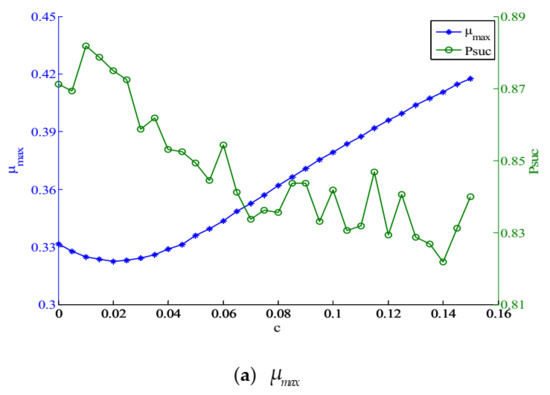
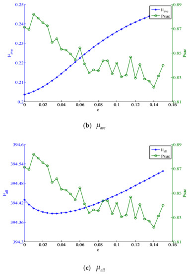
Figure 1. (a) ${\mu }_{max}$ and $P_{suc}$ versus $c$; (b) ${\mu }_{ave}$ and $P_{suc}$ versus $c$; (c) ${\mu }_{all}$ and $P_{suc}$ versus $c$, both with $M=28$ and $K=8$.

When $c=0$, the shrinkage function shown as (7) is the same as (6). As can be seen from the graphs, when $c$ increases, ${\mu }_{ave}$ increases, ${\mu }_{max}$ and ${\mu }_{all}$ decrease first and then increase, $P_{suc}$ increases firstly and then decreases. ${\mu }_{max}$ and ${\mu }_{all}$ reach the minima when $c=0.02$ and $c=0.03$ respectively. It is worth noting that appropriate increase of $c$ leads to decrease of ${\mu }_{max}$ and ${\mu }_{all}$ but increase of ${\mu }_{ave}$. When $c=0.01$, better ${\mu }_{max}$ and ${\mu }_{all}$ are obtained and the loss in ${\mu }_{ave}$ is tolerable. Moreover, $P_{suc}$ reaches the maxima. Therefore, 0.01 may be a moderate value for $c$ and $c$ is set to 0.01 in the simulations in Section 4.2, Section 4.3 and Section 4.4.

4.2. Comparing the Mutual Coherence Indexes

This section presents a series of simulations to compare our method with algorithms given in [8,16,17] on the three mutual coherence indexes of $\mathit{D}$ obtained by $\mathit{D}={\mathit{\Phi }}_{opt}\mathit{\Psi }$ where ${\mathit{\Phi }}_{opt}$ is the optimized measurement matrix. For convenience, each method is denoted as Propose, Elad, Hong, and Entezari. The down-scaling factor for Elad is set to 0.95. The inner iteration number for Hong is set to 2, which means K-SVD is applied twice in every updating of $\mathit{\Phi }$. The point is set to 0.5 to update the ${\mathit{G}}_t$ in Entezari.

Figure 2 illustrates the change tendency of mutual coherence indexes with iteration number for $M=28$. As can be seen from the figure, the indexes corresponding to different algorithms all change monotonously with the iteration number. When ${\mu }_{max}$ and ${\mu }_{ave}$ converge, the number of iterations required by our method is almost equal to that of Hong and significantly less than that of Elad. When ${\mu }_{all}$ converges, the number of iterations required by our method is equivalent to that of Entezari and significantly less than that of Hong and Elad.

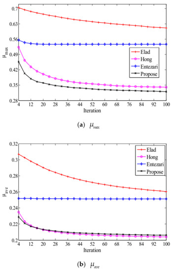
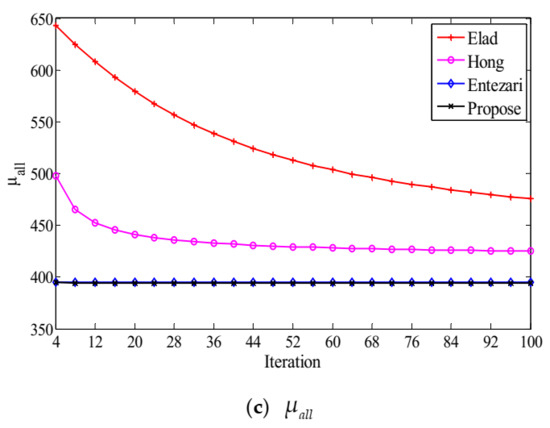
Figure 2. The convergence results: (a) evolution of ${\mu }_{max}$, (b) ${\mu }_{ave}$ and (c) the evolution of ${\mu }_{all}$, all versus iteration number, where $M=28$.

Figure 3 presents the histogram of the absolute off-diagonal values of ${\left({\mathit{\Phi }}_{opt}\mathit{\Psi }\right)}^{\prime }{\mathit{\Phi }}_{opt}\mathit{\Psi }$ for $M=28$. It is seen from the figure that Elad and Entezari have long tails, showing that the number of off-diagonal values that exceed 0.34 is relatively large. The tail of Hong is shorter than that of Elad and Entezari, and reaches the maximum of 0.34. Compared with Hong, our method has a shorter tail which reaches the maximum of 0.32 and has more off-diagonal values below the ${\mu }_{welch}$ (0.1662).

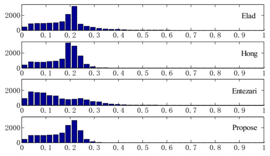
Figure 3. Histogram of the absolute off-diagonal values of ${\left({\mathit{\Phi }}_{opt}\mathit{\Psi }\right)}^{\prime }{\mathit{\Phi }}_{opt}\mathit{\Psi }$ for $M=28$.

Table 1, Table 2 and Table 3 present ${\mu }_{max}$, ${\mu }_{ave}$, and ${\mu }_{all}$ by Elad, Hong, Entezari, and our method versus measurement dimension $M$ respectively. From Table 1, it can be observed that the ${\mu }_{max}$ of our method is significantly less than that of Elad and Entezari, and less than Hong, which means our method is effective in reducing the maximum mutual coherence. In Table 2, we see that the ${\mu }_{ave}$ of our method is significantly less than that of Elad and Entezari, with an advantage of more than 0.03. It is worth noting that the ${\mu }_{ave}$ of our method is slightly larger than Hong. In Table 3, the ${\mu }_{all}$ of our method is significantly less than that of Elad and Hong, with an advantage of more than 70 and 20 respectively. On the other hand, the ${\mu }_{all}$ of our method is almost the same as Entezari.

Table 1. ${\mu }_{max}$ by Elad, Hong, Entezari, and proposed method versus measurement dimension $M$.

M	Elad	Hong	Entezari	Propose	${\mathit{\mu }}_{\mathit{w}\mathit{e}\mathit{l}\mathit{c}\mathit{h}}$
12	0.8971	0.8884	0.8465	0.8072	0.2750
16	0.8157	0.6488	0.7517	0.5211	0.2337
20	0.7610	0.4625	0.6710	0.4218	0.2050
24	0.6972	0.3920	0.5874	0.3618	0.1833
28	0.6186	0.3403	0.5351	0.3223	0.1662
32	0.5460	0.3069	0.4911	0.2919	0.1520
36	0.4879	0.2804	0.4472	0.2659	0.1400
40	0.4454	0.2591	0.4177	0.2487	0.1296
44	0.3802	0.2404	0.3927	0.2302	0.1205

Table 2. ${\mu }_{ave}$ by Elad, Hong, Entezari, and proposed method versus measurement dimension $M$.

M	Elad	Hong	Entezari	Propose	${\mu }_{welch}$
12	0.4168	0.4528	0.4141	0.3608	0.2750
16	0.3507	0.2964	0.3532	0.2979	0.2337
20	0.3016	0.2566	0.3111	0.2581	0.2050
24	0.2431	0.2272	0.2772	0.2288	0.1833
28	0.2212	0.2042	0.2512	0.2060	0.1662
32	0.2056	0.1854	0.2302	0.1879	0.1520
36	0.1937	0.1700	0.2118	0.1727	0.1400
40	0.1841	0.1567	0.1961	0.1600	0.1296
44	0.1760	0.1454	0.1824	0.1491	0.1205

Table 3. ${\mu }_{all}$ by Elad, Hong, Entezari, and proposed method versus measurement dimension $M$.

M	Elad	Hong	Entezari	Propose
12	1220.20	2638.47	1081.18	1080.19
16	898.80	802.77	780.92	780.16
20	721.41	630.91	605.72	600.13
24	571.34	512.24	480.67	480.12
28	474.76	425.25	394.86	394.39
32	404.35	358.49	330.55	330.11
36	353.96	307.11	280.55	280.10
40	315.03	265.40	240.55	240.10
44	285.51	231.43	207.79	207.38

In conclusion, while effectively reducing ${\mu }_{max}$ and ${\mu }_{all}$, our method can maintain a small ${\mu }_{ave}$ at the same time. Additionally, the number of iterations required for the convergence of each index of our method is significantly less than that of Elad. Therefore, from the view of mutual coherence indexes, the measurement matrix obtained by our method has better properties than the other three methods. This coincides with the theoretical results obtained in the Section 3.

4.3. Comparing the Reconstruction Performance

Case 1.

Comparison of the$P_{suc}$in the noiseless case.

In this case, we conduct two separate CS experiments, first by fixing $K=8$ and varying $M$ from 12 to 44 and second by fixing $M=28$ and varying $K$ from 4 to 20. Each experiment is performed for 1000 random sparse ensembles and the number of exact reconstruction is recorded.

Figure 4 and Figure 5 reveal that the $P_{suc}$ of our method is the highest, which indicates its superiority over the other three methods.

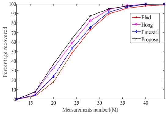
Figure 4. The change tendency of $P_{suc}$ with $M$ while $K=8$ in the noiseless case.

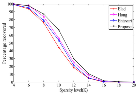
Figure 5. The change tendency of $P_{suc}$ with $K$ while $M=28$ in the noiseless case.

Case 2.

Comparison of the$\epsilon$in the noisy case.

To show the robustness of the proposed method in noisy cases we consider the noisy model $y=\mathit{\Phi }x+v$ where $v$ is the vector of additive Gaussian noise with zero means. We conduct the experiment by fixing $M=28$, $K=8$, and varying SNR from 10 to 50 dB. The experiment is performed for 1000 random sparse ensembles and the average reconstruction error is recorded. From Figure 6, we can see that the reconstruction errors decrease with the increase of SNR, and the error of the proposed method is smaller than that of the others.

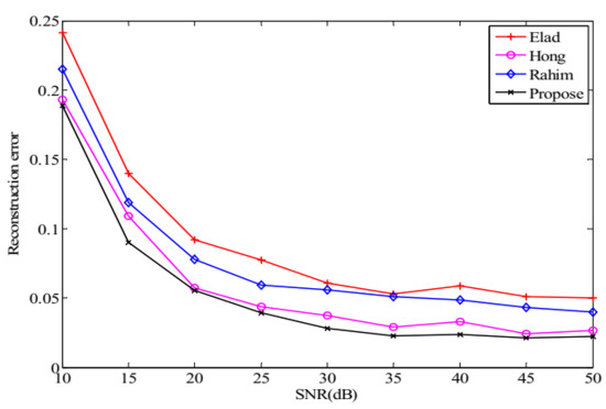
Figure 6. The change tendency of $\epsilon$ with SNR while $M=40$ and $K=8$.

Table 3 presents that ${\mu }_{all}$ of the Entezari is slightly larger than that of our method. It is interesting to note that the number of off-diagonal entries with smaller absolute values in the Entezari is significantly larger than that of our method from Figure 3. Moreover, it can be seen from Table 2 that ${\mu }_{ave}$ of Hong is slightly lower than that of our method. However, the simulation results show that our method outperforms the others in terms of reconstruction performance. It is also worthy noting that our method reduces ${\mu }_{ave}$, ${\mu }_{max}$, and ${\mu }_{all}$ simultaneously, leading to better reconstruction performance in CS. This implies that a single mutual coherence index cannot accurately reflect the actual performance of the methods, and verifies the necessity of using multiple indexes simultaneously in measurement matrix optimization.

4.4. Different Kinds of $\mathit{\Phi }$ and $\mathit{\Psi }$ Optimized by the Proposed Methods

To analyze the performance of our method with various measurement matrices and dictionary matrices, a serious of simulations are carried out in this section. We choose the measurement matrix as a Gaussian random matrix and a Bernoulli random matrix, and choose the dictionary matrix as a Gaussian random matrix and the DCT matrix, respectively. We compare the mutual coherence indexes and the reconstruction performance before and after optimization. When $\mathit{\Psi }$ is the Gaussian random matrix, $\mathit{\Phi }$ belongs to ${\mathrm{R}}^{\mathrm{M}\times 80}$ and $\mathit{\Psi }$ belongs to ${\mathrm{R}}^{80\times 120}$. When $\mathit{\Psi }$ is the DCT matrix, $\mathit{\Phi }$ belongs to ${\mathrm{R}}^{\mathrm{M}\times 120}$ and $\mathit{\Psi }$ belongs to ${\mathrm{R}}^{120\times 120}$. Each experiment is performed for 1000 random sparse ensembles.

The mutual coherence indexes of different measurement matrices $\mathit{\Phi }$ with different dictionary matrices $\mathit{\Psi }$ are shown in Figure 7. As seen from the simulations, all the optimized measurement matrices produce smaller ${\mu }_{max}$, ${\mu }_{ave}$, and ${\mu }_{all}$ than the random ones.

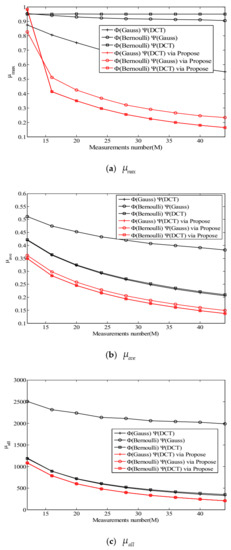
Figure 7. The evolution of (a) ${\mu }_{max}$, (b) ${\mu }_{ave}$ and (c) ${\mu }_{all}$, all versus measurements number with different $\mathit{D}$.

Figure 8 and Figure 9 present the reconstruction performance of OMP with the optimized measurement matrices and the random ones. It is seen from the graphs in these figures that all the optimized matrices outperform the random ones in terms of the percentage of exact reconstruction.

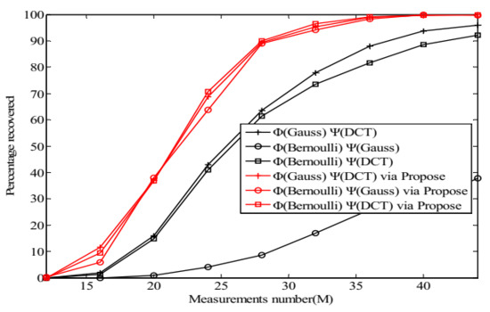
Figure 8. The change tendency of $P_{suc}$ with $M$ while $K=8$ in the noiseless case.

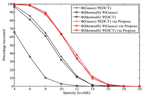
Figure 9. The change tendency of $P_{suc}$ with $K$ while $M=28$ in the noiseless case.

5. Conclusions

This paper focused on the optimization of measurement matrix for compressed sensing. To decrease ${\mu }_{max}$, ${\mu }_{ave}$, and ${\mu }_{all}$ simultaneously, we designed a new target Gram matrix which was obtained by applying a new shrinkage function to the Gram matrix and updated by performing rank reduction and eigenvalue averaging. Then, we characterized the analytical solutions of the measurement matrix by SVD. Based on alternating minimization, we proposed an iterative method to optimize the measurement matrix. The simulation results show that the proposed method reduces ${\mu }_{max}$, ${\mu }_{ave}$, and ${\mu }_{all}$ simultaneously and outperforms the existing algorithms in terms of reconstruction performance. In addition, the proposed method is computationally less expensive than some existing algorithms in the literature.

As detailed, we gave the optimal value of $c$ under a fixed matrix scale through simulation. When the scale changes, the value of $c$ in Section 4.1 may no longer be applicable. Therefore, it is meaningful to find the theoretical ‘optimal value’ of $c$. Furthermore, noting that lower mutual coherence indexes mean potentially higher reconstruction performance, further efforts are needed to decrease the indexes simultaneously.

References

- Donoho, D.L. Compressed sensing. IEEE Trans. Inf. Theory 2006, 52, 1289–1306. [Google Scholar] [CrossRef]
- Xie, Y.; Yu, J.; Guo, S.; Ding, Q.; Wang, E. Image Encryption Scheme with Compressed Sensing Based on New Three-Dimensional Chaotic System. Entropy 2019, 21, 819. [Google Scholar] [CrossRef]
- Fang, Y.; Li, L.; Li, Y.; Peng, H.; Yang, Y. Low Energy Consumption Compressed Spectrum Sensing Based on Channel Energy Reconstruction in Cognitive Radio Network. Sensors 2020, 20, 1264. [Google Scholar] [CrossRef]
- Martinez, J.A.; Ruiz, P.M.; Skarmeta, A.F. Evaluation of the Use of Compressed Sensing in Data Harvesting for Vehicular Sensor Networks. Sensors 2020, 20, 1434. [Google Scholar] [CrossRef]
- Donoho, D.L.; Elad, M. Optimally sparse representation in general (nonorthogonal) dictionaries via 1 minimization. Proc. Natl. Acad. Sci. USA 2003, 100, 2197–2202. [Google Scholar] [CrossRef]
- Candes, E.J.; Tao, T. Decoding by linear programming. IEEE Trans. Inf. Theory 2005, 51, 4203–4215. [Google Scholar] [CrossRef]
- Stark, D.P.B. Uncertainty Principles and Signal Recovery. SIAM J. Appl. Math. 1989, 49, 906–931. [Google Scholar]
- Elad, M. Optimized Projections for Compressed Sensing. IEEE Trans. Signal Process. 2007, 55, 5695–5702. [Google Scholar] [CrossRef]
- Shaohai, H.U. An Optimization Method for Measurement Matrix Based on Eigenvalue Decomposition. Signal Process. 2012. [Google Scholar] [CrossRef]
- Yan, W.; Wang, Q.; Shen, Y. Shrinkage-Based Alternating Projection Algorithm for Efficient Measurement Matrix Construction in Compressive Sensing. IEEE Trans. Instrum. Meas. 2014, 63, 1073–1084. [Google Scholar] [CrossRef]
- Duartecarvajalino, J.M.; Sapiro, G. Learning to Sense Sparse Signals: Simultaneous Sensing Matrix and Sparsifying Dictionary Optimization. IEEE Trans. Image Process. 2009, 18, 1395–1408. [Google Scholar] [CrossRef]
- Lu, C.; Li, H.; Lin, Z. Optimized Projections for Compressed Sensing via Direct Mutual Coherence Minimization. Signal Process. 2018, 151, 45–55. [Google Scholar] [CrossRef]
- Xu, J.; Pi, Y.; Cao, Z. Optimized projection matrix for compressive sensing. EURASIP J. Adv. Signal Process. 2010, 2010, 560349. [Google Scholar] [CrossRef]
- Abolghasemi, V.; Ferdowsi, S.; Sanei, S. A gradient-based alternating minimization approach for optimization of the measurement matrix in compressive sensing. Signal Process. 2012, 92, 999–1009. [Google Scholar] [CrossRef]
- Zheng, H.; Li, Z.; Huang, Y. An Optimization Method for CS Projection Matrix Based on Quasi-Newton Method. Acta Electron. Sin. 2014, 42, 1977–1982. [Google Scholar]
- Hong, T.; Bai, H.; Li, S.; Zhu, Z. An efficient algorithm for designing projection matrix in compressive sensing based on alternating optimization. Signal Process. 2016, 125, 9–20. [Google Scholar] [CrossRef]
- Entezari, R.; Rashidi, A. Measurement matrix optimization based on incoherent unit norm tight frame. AEU Int. J. Electron. Commun. 2017, 82, 321–326. [Google Scholar] [CrossRef]
- Sustik, M.A.; Tropp, J.A.; Dhillon, I.S.; Heath, R.W. On the existence of equiangular tight frames. Linear Algebra Its Appl. 2007, 426, 619–635. [Google Scholar] [CrossRef]
- Welch, L. Lower bounds on the maximum cross correlation of signals (Corresp.). IEEE Trans. Inf. Theory 1974, 20, 397–399. [Google Scholar] [CrossRef]
- Aharon, M.; Elad, M.; Bruckstein, A.M. K-SVD: An Algorithm for Designing Overcomplete Dictionaries for Sparse Representation. IEEE Trans. Signal Process. 2006, 54, 4311–4322. [Google Scholar] [CrossRef]
- Fickus, M.; Mixon, D.G. Tables of the existence of equiangular tight frames. arXiv 2015, arXiv:1504.00253. [Google Scholar]
- Li, G.; Zhu, Z.; Yang, D.; Chang, L.; Bai, H. On Projection Matrix Optimization for Compressive Sensing Systems. IEEE Trans. Signal Process. 2013, 61, 2887–2898. [Google Scholar] [CrossRef]
- Tropp, J.A.; Gilbert, A.C. Signal Recovery from Random Measurements Via Orthogonal Matching Pursuit. IEEE Trans. Inf. Theory 2007, 53, 4655–4666. [Google Scholar] [CrossRef]
Publisher’s Note: MDPI stays neutral with regard to jurisdictional claims in published maps and institutional affiliations. |
© 2021 by the authors. Licensee MDPI, Basel, Switzerland. This article is an open access article distributed under the terms and conditions of the Creative Commons Attribution (CC BY) license (http://creativecommons.org/licenses/by/4.0/).