
An SVEIRE Model of Tuberculosis to Assess the Effect of an Imperfect Vaccine and Other Exogenous Factors


Abstract
1. Introduction
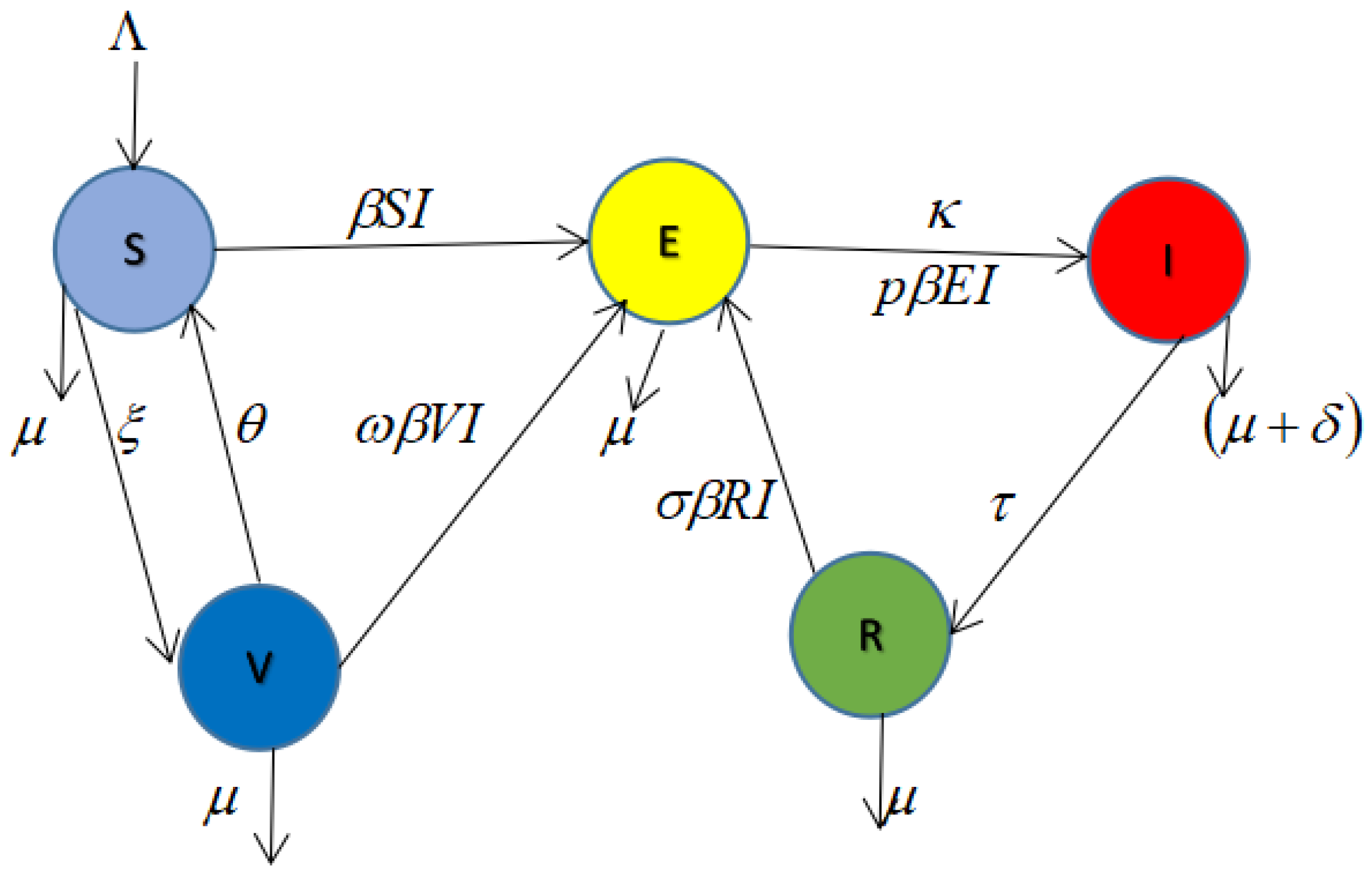
2. Model and Methods
Biological Assumptions of the Model
- There is a constant recruitment rate to the susceptible population and natural cause death affects individuals in all compartments, with an extra TB-induced death rate in the infected class;
- Some susceptible individuals who have been successfully vaccinated lose their vaccine-induced immunity (i.e., vaccine failed), and these previously vaccinated individuals join the susceptible compartment again [38].
- The individuals in the susceptible class move to the exposed class with the transmission rate
- The individuals in the exposed class become infectious and move to the infected class. After recovery, they move to the recovered compartment. When the recovered individuals loose immunity, they return to the exposed class [21].
3. Mathematical Model Analysis
3.1. Positivity of Solutions
3.2. Invariant Region
4. Analysis of Disease-Free Equilibrium (), , and Basic Reproduction Number
4.1. Basic Reproduction Number ()
4.2. Proving the Local Stability of Disease-Free Equilibrium Point
- (i)
- Tr(A)
- (ii)
- Det (A) .
5. Endemic Equilibrium and Bifurcation Analysis
- A unique endemic equilibrium when and cases 1–3 are satisfied;
- One or more than one endemic equilibrium when and cases 5–7 are satisfied; and
- No endemic equilibrium when and case 8 shows that all the coefficients are positive.
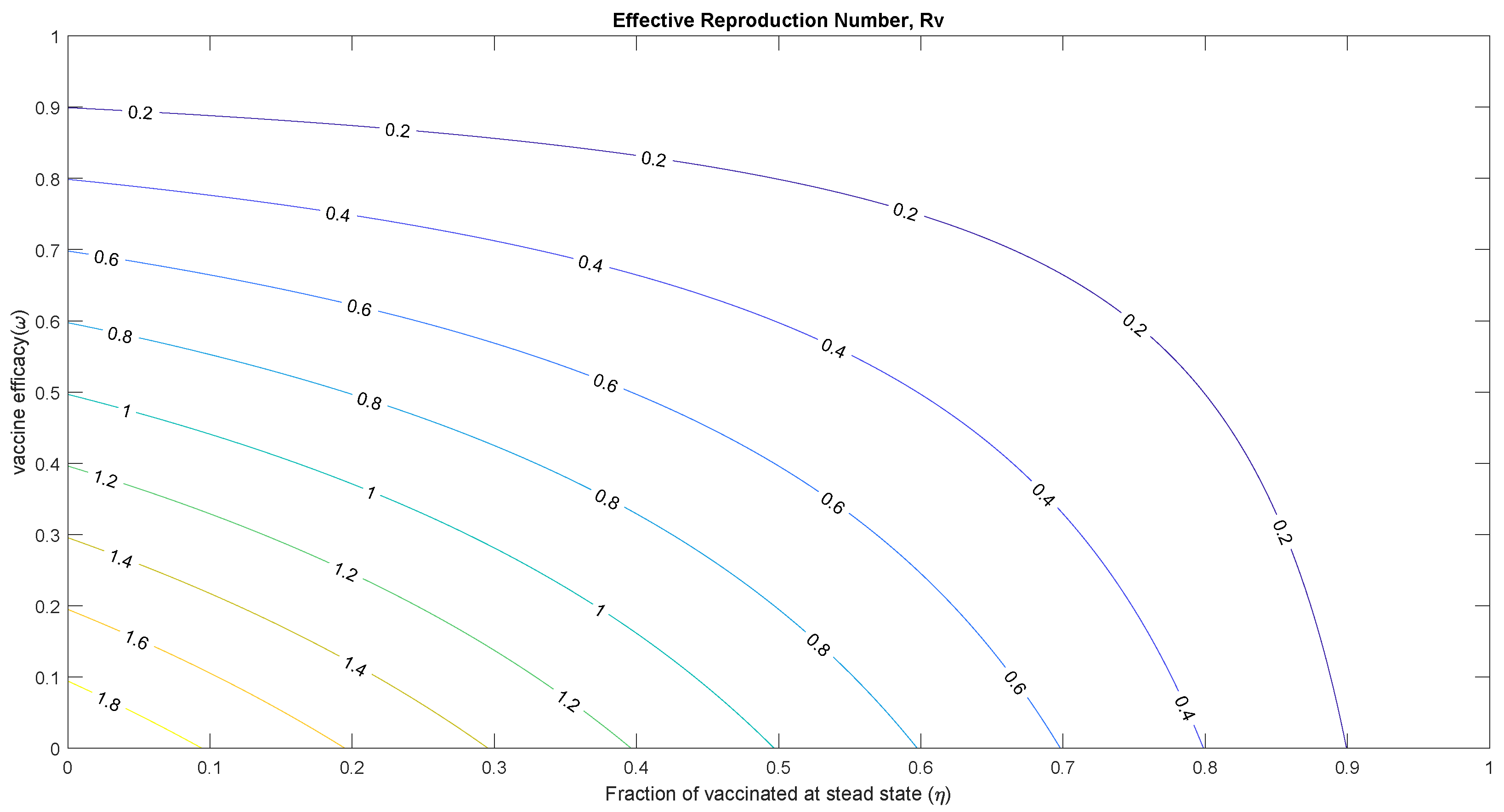
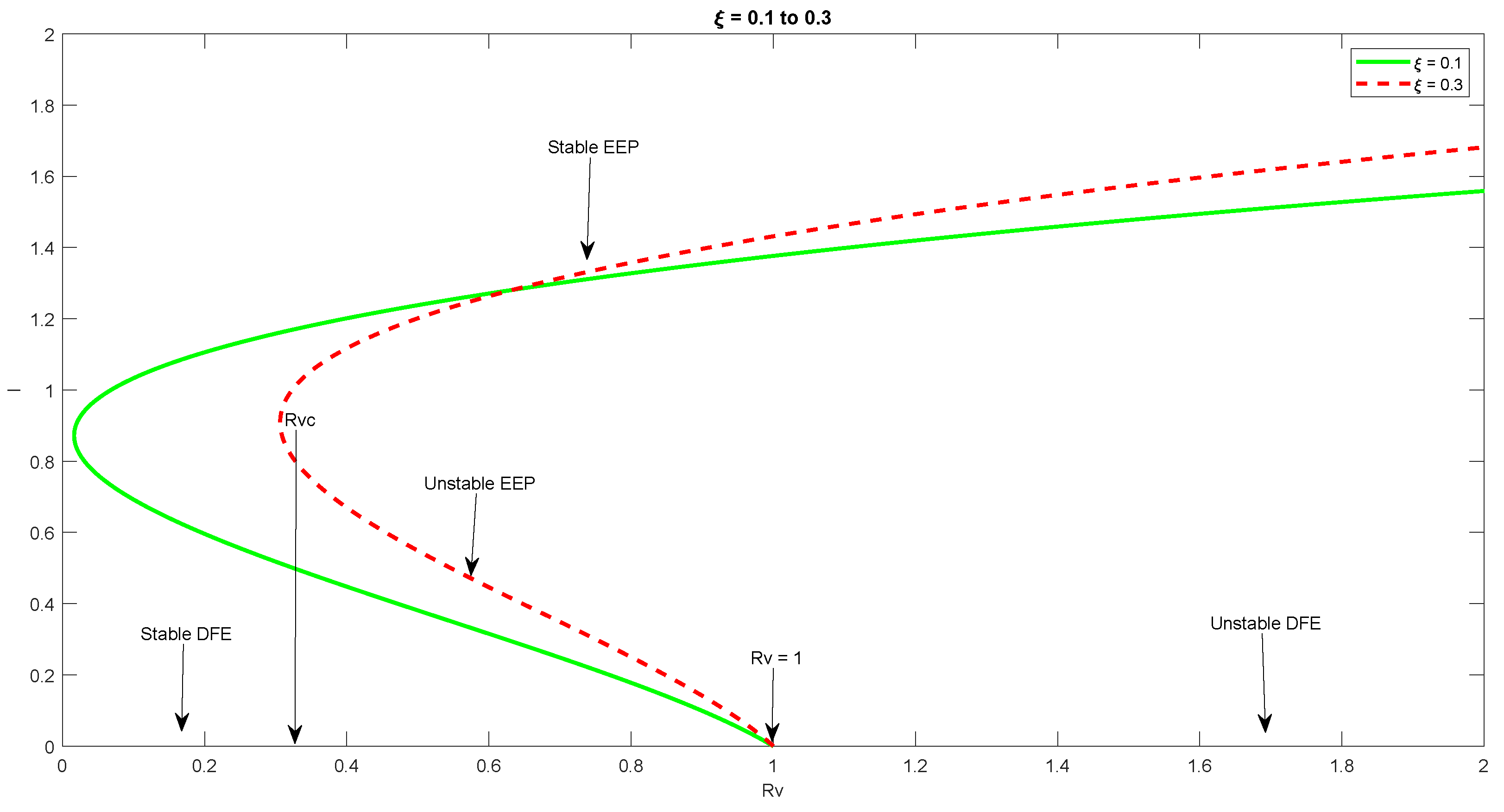
5.1. Threshold Analysis and Vaccine Impact
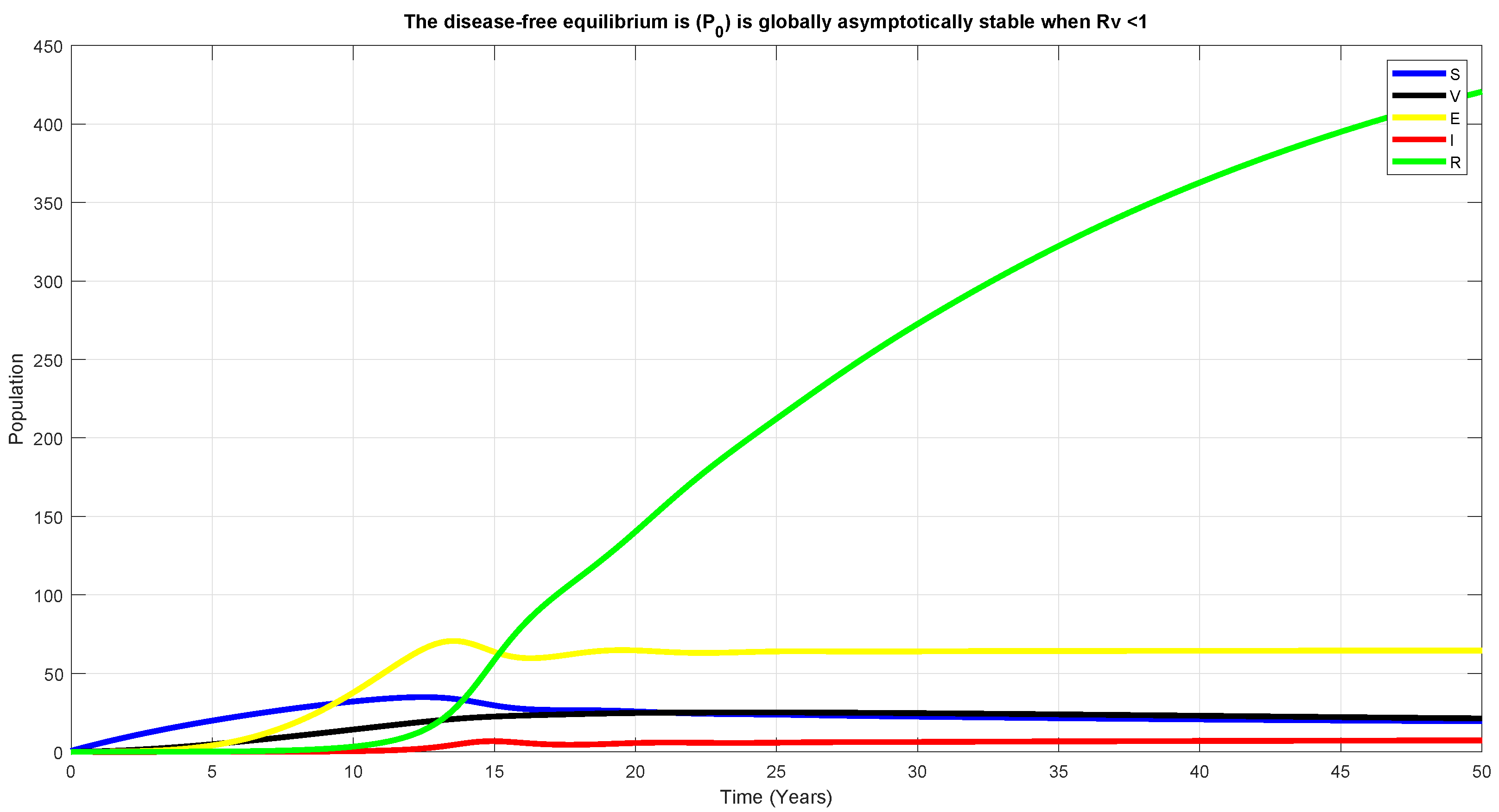
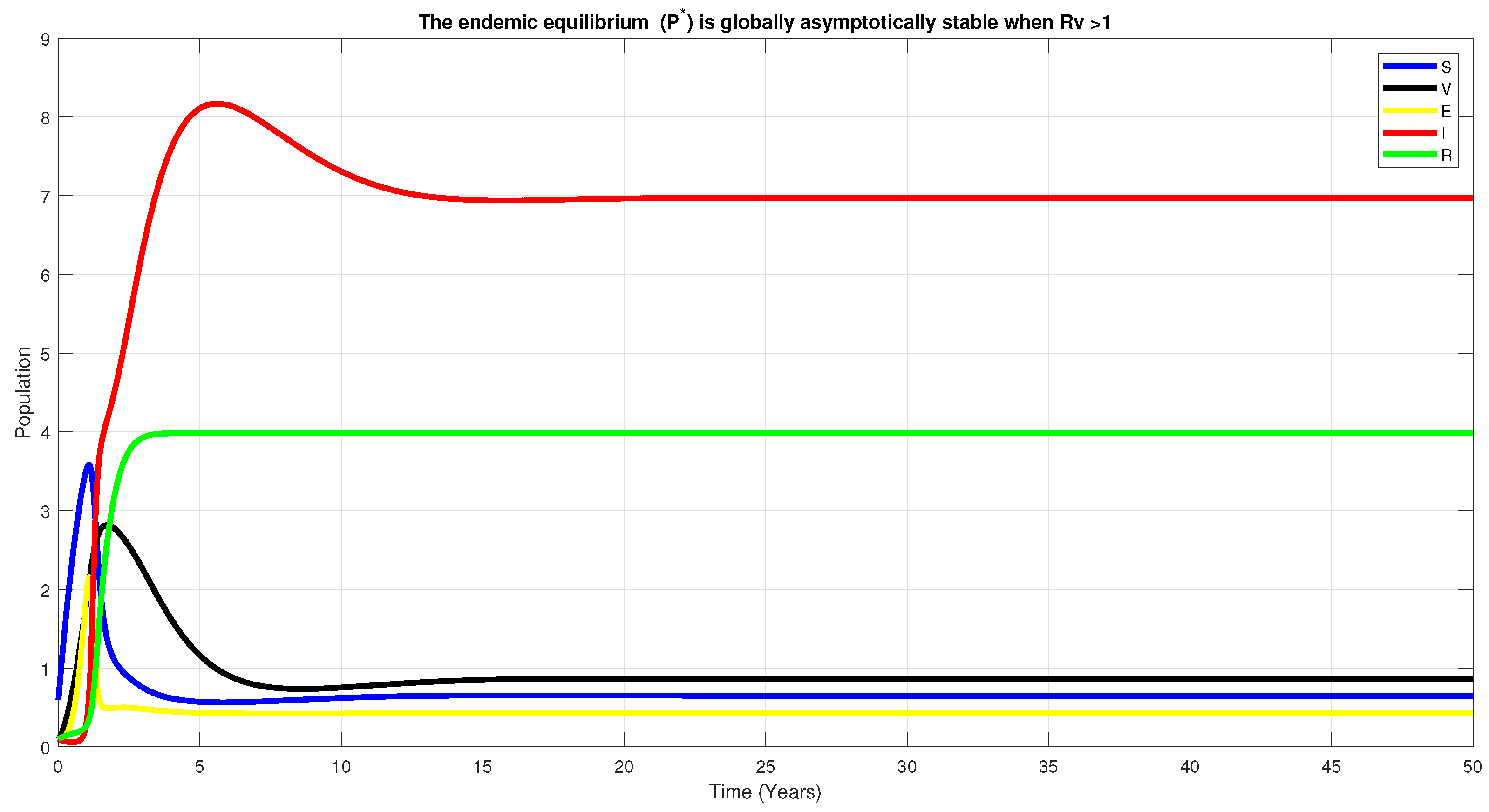
5.2. Global Stability of DFE, , for
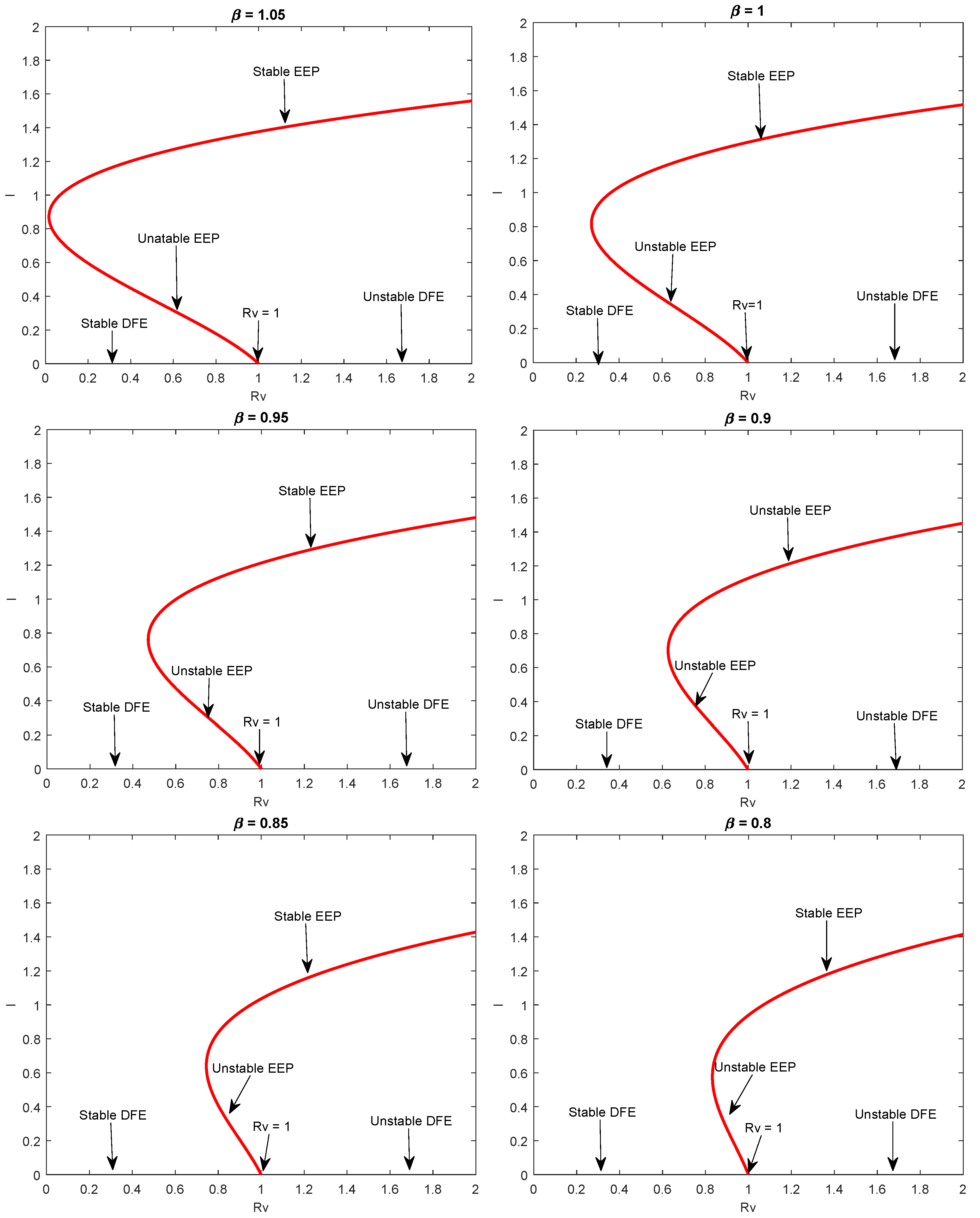
5.3. Analysis of Backward Bifurcation
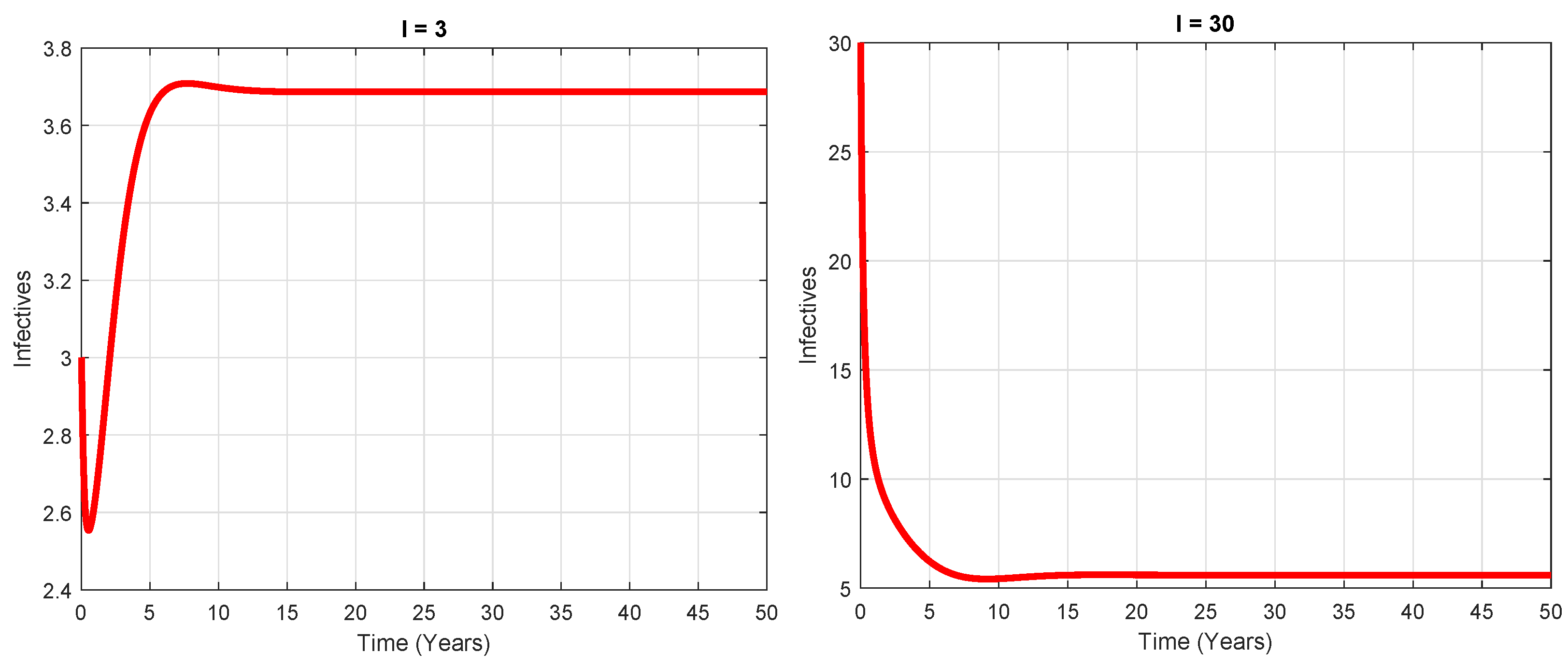
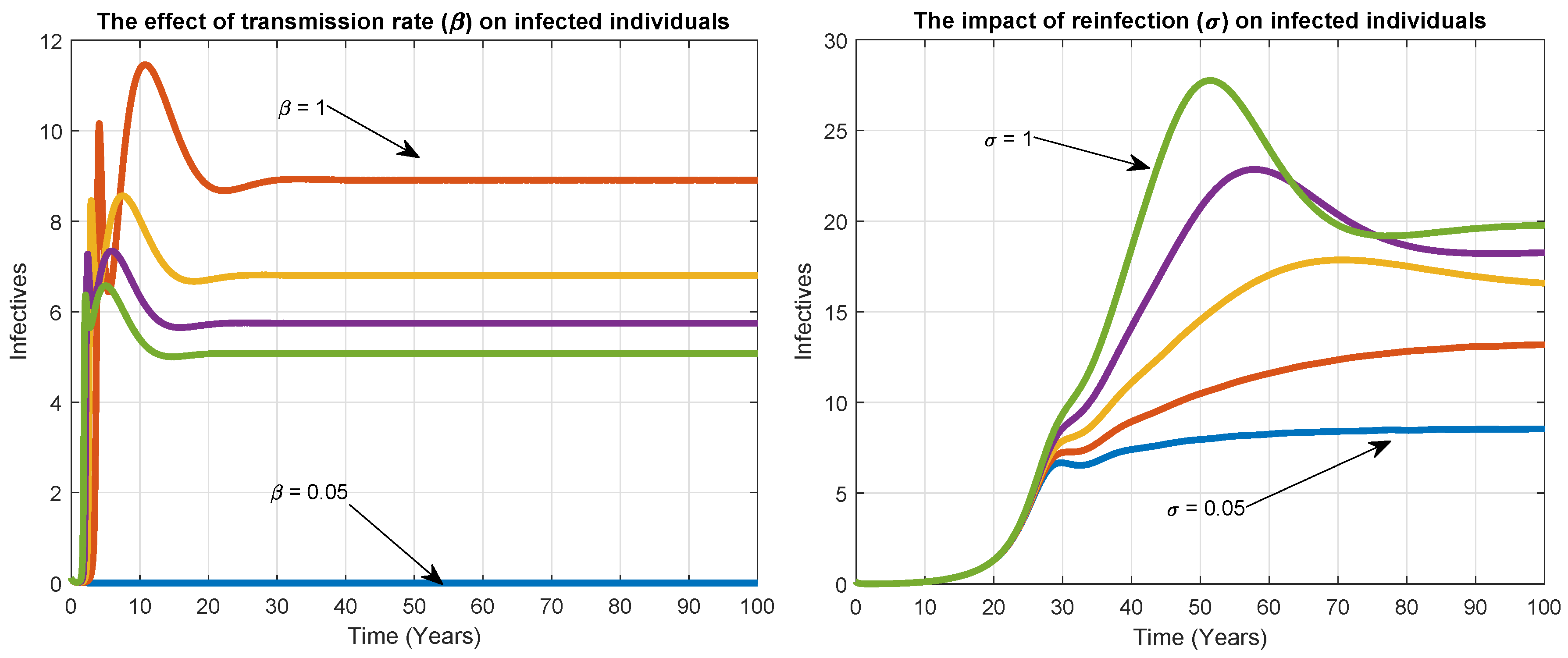
6. Numerical Simulation
7. Discussion
8. Conclusions
Author Contributions
Funding
Institutional Review Board Statement
Informed Consent Statement
Data Availability Statement
Acknowledgments
Conflicts of Interest
References
- World Health Organization. Global Tuberculosis Report; WHO: Geneva, Switzerland, 2018; p. 214. [Google Scholar]
- Khajanchi, S.; Das, D.K.; Kar, T.K. Dynamics of tuberculosis transmission with exogenous reinfections and endogenous reactivation. Phys. A 2018, 497, 52–71. [Google Scholar] [CrossRef]
- Ullah, S.; Khan, M.A.; Farooq, M.; Gul, T. Modeling and analysis of Tuberculosis (TB) in Khyber Pakhtunkhwa, Pakistan. Math. Comput. Simul 2019, 165, 181–199. [Google Scholar] [CrossRef]
- Bloom, B.R.; Murray, C.J. Tuberculosis: Commentary on a reemergent killer. Science 1992, 257, 1055–1064. [Google Scholar] [CrossRef]
- Hill, A.N.; Becerra, J.E.; Castro, K.G. Modelling tuberculosis trends in the USA. Epidemiol. Infect. 2012, 257, 1862–1872. [Google Scholar] [CrossRef]
- Abubakar, I.; Dara, M.; Manissero, D.; Zumla, A. Tackling the spread of drug-resistant tuberculosis in Europe. Lancet 2012, 379, e21–e23. [Google Scholar] [CrossRef]
- Behr, M.A. Tuberculosis Due to Multiple Strains: A Concern for the Patient? A Concern for Tuberculosis Control? Ann. Am. Thorac. Soc. 2004, 169, 554–555. [Google Scholar] [CrossRef]
- Fatima, S.; Kumari, A.; Das, G.; Dwivedi, V.P. Tuberculosis vaccine: A journey from BCG to present. Life Sci. 2020, 252, 117594. [Google Scholar] [CrossRef]
- Sudre, P.; Ten Dam, G.; Kochi, A. Tuberculosis: A global overview of the situation today. Bull. World Health Org. 1992, 70, 149. [Google Scholar]
- Dolin, P.J.; Raviglione, M.C.; Kochi, A. Global tuberculosis incidence and mortality during 1990–2000. Bull. World Health Org. 1994, 72, 213. [Google Scholar]
- Moghadas, S.M.; Alexander, M.E. Exogenous reinfection and resurgence of tuberculosis: A theoretical framework. J. Biol. Syst. 2004, 12, 231–247. [Google Scholar] [CrossRef]
- Castillo-Chavez, C.; Song, B. Dynamical models of tuberculosis and their applications. Math. Biosci. Eng. 2004, 1, 361. [Google Scholar] [CrossRef] [PubMed]
- Adebiyi, A.O. Mathematical Modeling of the Population Dynamics of Tuberculosis; University of the Western Cape: Cape Town, South Africa, 2016. [Google Scholar]
- Richardson, M.; Carroll, N.M.; Engelke, E.; van der Spuy, G.D.; Salker, F.; Munch, Z.; van Helden, P.D. Multiple Mycobacterium tuberculosis strains in early cultures from patients in a high-incidence community setting. J. Clin. Microbiol. 2002, 40, 2750–2754. [Google Scholar] [CrossRef] [PubMed][Green Version]
- Reichman, L.B.; Hershfield, E.S. Tuberculosis: A Comprehensive International Approach; CRC Press: Boca Raton, FL, USA, 2000. [Google Scholar]
- Lin, P.L.; Ford, C.B.; Coleman, M.T.; Myers, A.J.; Gawande, R.; Ioerger, T.; Flynn, J.L. Sterilization of granulomas is common in active and latent tuberculosis despite within-host variability in bacterial killing. Nat. Med. 2014, 20, 75–79. [Google Scholar] [CrossRef] [PubMed]
- Smith, P.G.; Moss, A.R. Epidemiology of tuberculosis. In Tuberculosis; American Society for Microbiology: Washington, DC, USA, 1994; pp. 47–59. [Google Scholar]
- Blower, S.M.; Mclean, A.R.; Porco, T.C.; Small, P.M.; Hopewell, P.C.; Sanchez, M.A.; Moss, A.R. The intrinsic transmission dynamics of tuberculosis epidemics. Nat. Med. 1995, 1, 815–821. [Google Scholar] [CrossRef] [PubMed]
- Vynnycky, E.; Fine, P.E. Lifetime risks, incubation period, and serial interval of tuberculosis. Am. J. Epidemiol. 2000, 152, 247–263. [Google Scholar] [CrossRef]
- Drain, P.K.; Bajema, K.L.; Dowdy, D.; Dheda, K.; Naidoo, K.; Schumacher, S.G.; Sherman, D.R. Incipient and subclinical tuberculosis: A clinical review of early stages and progression of infection. Clin. Microbiol. Rev. 2018, 31. [Google Scholar] [CrossRef]
- Kar, T.K.; Mondal, P.K. Global dynamics of a tuberculosis epidemic model and the influence of backward bifurcation. J. Math. Model. Algorithms 2012, 11, 433–459. [Google Scholar] [CrossRef]
- Wangari, I.M.; Davis, S.; Stone, L. Backward bifurcation in epidemic models: Problems arising with aggregated bifurcation parameters. Appl. Math. Model. 2016, 40, 1669–1675. [Google Scholar] [CrossRef]
- Cohen, T.; Colijn, C.; Finklea, B.; Murray, M. Exogenous re-infection and the dynamics of tuberculosis epidemics: Local effects in a network model of transmission. J. R. Soc. Interface 2007, 4, 523–531. [Google Scholar] [CrossRef]
- Gomes, M.G.M.; Rodrigues, P.; Hilker, F.M.; Mantilla-Beniers, N.B.; Muehlen, M.; Paulo, A.C.; Medley, G.F. Implications of partial immunity on the prospects for tuberculosis control by post-exposure interventions. J. Theor. Biol. 2007, 248, 608–617. [Google Scholar] [CrossRef][Green Version]
- Liu, X.; Takeuchi, Y.; Iwami, S. SVIR epidemic models with vaccination strategies. J. Theor. Biol. 2008, 253, 1–11. [Google Scholar] [CrossRef] [PubMed]
- Anderson, R.M.; Anderson, B.; Robert, M.M. Infectious Diseases of Humans: Dynamics and Control; Oxford University Press: Oxford, UK, 1992. [Google Scholar]
- Buonomo, B.; Lacitignola, D. On the backward bifurcation of a vaccination model with nonlinear incidence. Nonlinear Anal. Model. Control 2011, 16, 30–46. [Google Scholar] [CrossRef]
- Buonomo, B.; Della Marca, R. Oscillations and hysteresis in an epidemic model with information-dependent imperfect vaccination. Math. Comput. Simul. 2019, 162, 97–114. [Google Scholar] [CrossRef]
- Andersen, P.; Doherty, T.M. The success and failure of BCG—Implications for a novel tuberculosis vaccine. Nat. Rev. Microbiol. 2005, 3, 656–662. [Google Scholar] [CrossRef] [PubMed]
- Nadolinskaia, N.I.; Karpov, D.S.; Goncharenko, A.V. Vaccines against Tuberculosis: Problems and Prospects. Appl. Biochem. Microbiol. 2020, 56, 497–504. [Google Scholar] [CrossRef]
- Fine, P.E.; Carneiro, I.A.; Milstien, J.B.; Clements, C.J. Issues Relating to the Use of BCG in Immunization Programmes: A Discussion Document (No. WHO/V and B/99.23); World Health Organization: Geneva, Switzerland, 1999. [Google Scholar]
- van Rie, A.; Warren, R.; Richardson, M.; Victor, T.C.; Gie, R.P.; Enarson, D.A.; van Helden, P.D. Exogenous reinfection as a cause of recurrent tuberculosis after curative treatment. N. Engl. J. Med. 1999, 341, 1174–1179. [Google Scholar] [CrossRef]
- Bhunu, C.P.; Garira, W.; Mukandavire, Z.; Zimba, M. Tuberculosis transmission model with chemoprophylaxis and treatment. Bull. Math. Biol. 2008, 70, 1163–1191. [Google Scholar]
- Feng, Z.; Castillo-Chavez, C.; Capurro, A.F. A model for tuberculosis with exogenous reinfection. Theor. Popul. Biol. 2000, 57, 235–247. [Google Scholar] [CrossRef]
- Song, B.; Castillo-Chavez, C.; Aparicio, J.P. Tuberculosis models with fast and slow dynamics: The role of close and casual contacts. Math. Biosci. 2002, 180, 187–205. [Google Scholar]
- Liu, S.; Li, Y.; Bi, Y.; Huang, Q. Mixed vaccination strategy for the control of tuberculosis: A case study in China. Math. Biosci. Eng. 2017, 14, 695. [Google Scholar]
- Renardy, M.; Kirschner, D.E. Evaluating vaccination strategies for tuberculosis in endemic and non-endemic settings. J. Theor. Biol 2019, 469, 1–11. [Google Scholar] [CrossRef]
- Gerberry, D.J. Practical aspects of backward bifurcation in a mathematical model for tuberculosis. J. Theor. Biol. 2016, 388, 15–36. [Google Scholar] [CrossRef]
- Nkamba, L.N.; Manga, T.T.; Agouanet, F.; Mann Manyombe, M.L. Mathematical model to assess vaccination and effective contact rate impact in the spread of tuberculosis. J. Biol. Dyn. 2019, 13, 26–42. [Google Scholar] [CrossRef]
- Egonmwan, A.O.; Okuonghae, D. Mathematical analysis of a tuberculosis model with imperfect vaccine. Int. J. Biomath. 2019, 12, 1950073. [Google Scholar] [CrossRef]
- Wangari, I. Backward Bifurcation and Reinfection in Mathematical Models of Tuberculosis. Ph.D. Thesis, RMIT University, Melbourne, Australia, 2017. [Google Scholar]
- Huang, W.; Cooke, K.L.; Castillo-Chavez, C. Stability and bifurcation for a multiple-group model for the dynamics of HIV/AIDS transmission. SIAM J. Appl. Math. 1992, 52, 835–854. [Google Scholar] [CrossRef]
- Hadeler, K.P.; Van den Driessche, P. Backward bifurcation in epidemic control. Math. Biosci. 1997, 146, 15–35. [Google Scholar] [CrossRef]
- Nudee, K.; Chinviriyasit, S.; Chinviriyasit, W. The effect of backward bifurcation in controlling measles transmission by vaccination. Chaos Soliton Fract. 2019, 123, 400–412. [Google Scholar] [CrossRef]
- Nadim, S.S.; Chattopadhyay, J. Occurrence of backward bifurcation and prediction of disease transmission with imperfect lockdown: A case study on COVID-19. Chaos Soliton Fract. 2019, 140, 110163. [Google Scholar] [CrossRef]
- Greenhalgh, D.; Diekmann, O.; de Jong, M.C. Subcritical endemic steady states in mathematical models for animal infections with incomplete immunity. Math. Biosci. 2000, 165, 1–25. [Google Scholar] [CrossRef]
- Gumel, A.B. Causes of backward bifurcations in some epidemiological models. J. Math. Anal. Appl. 2012, 395, 355–365. [Google Scholar]
- Hadeler, K.P.; Castillo-Chávez, C. A core group model for disease transmission. Math. Biosci. 1995, 128, 41–55. [Google Scholar] [CrossRef]
- Dushoff, J. Incorporating immunological ideas in epidemiological models. J. Theor. Biol. 1996, 180, 181–187. [Google Scholar] [CrossRef]
- Feng, Z.; Velasco-Hernandez, J.; Tapia-Santos, B. A mathematical model for coupling within-host and between-host dynamics in an environmentally-driven infectious disease. Math. Biosci. 2013, 241, 49–55. [Google Scholar] [CrossRef]
- Wang, W. Backward bifurcation of an epidemic model with treatment. Math. Biosci. 2006, 201, 58–71. [Google Scholar] [CrossRef]
- Cui, J.; Mu, X.; Wan, H. Saturation recovery leads to multiple endemic equilibria and backward bifurcation. J. Theor. Biol. 2008, 254, 275–283. [Google Scholar] [CrossRef]
- Hu, Z.; Ma, W.; Ruan, S. Analysis of SIR epidemic models with nonlinear incidence rate and treatment. Math. Biosci. 2013, 238, 12–20. [Google Scholar] [CrossRef]
- Dushoff, J.; Huang, W.; Castillo-Chavez, C. Backwards bifurcations and catastrophe in simple models of fatal diseases. J. Math. Biol. 1998, 36, 227–248. [Google Scholar] [CrossRef]
- Buonomo, B.; Vargas-De-León, C. Stability and bifurcation analysis of a vector-bias model of malaria transmission. Math. Biosci. 2013, 242, 59–67. [Google Scholar] [CrossRef]
- Gómez-Acevedo, H.; Li, M.Y. Backward bifurcation in a model for HTLV-I infection of CD4+ T cells. Bull. Math. Biol. 2005, 67, 101–114. [Google Scholar] [CrossRef]
- Martcheva, M.; Thieme, H.R. Progression age enhanced backward bifurcation in an epidemic model with super-infection. J. Math. Biol. 1998, 46, 385–424. [Google Scholar] [CrossRef]
- Omame, A.; Okuonghae, D.; Umana, R.A.; Inyama, S.C. Analysis of a co-infection model for HPV-TB. Appl. Math. Model. 2020, 77, 881–901. [Google Scholar] [CrossRef]
- Magpantay, F.M.; Riolo, M.A.; De Celles, M.D.; King, A.A.; Rohani, P. Epidemiological consequences of imperfect vaccines for immunizing infections. SIAM J. Appl. Math. 2014, 74, 1810–1830. [Google Scholar] [CrossRef] [PubMed]
- Gumel, A.B.; McCluskey, C.C.; Watmough, J. An SVEIR model for assessing potential impact of an imperfect anti-SARS vaccine. Math. Biosci. Eng. 2006, 3, 485. [Google Scholar] [PubMed]
- Moghadas, S.M. Modelling the effect of imperfect vaccines on disease epidemiology. Discrete. Continuous. Dyn. Syst. Ser. B 2004, 4, 999–1012. [Google Scholar] [CrossRef]
- Cai, L.M.; Li, Z.; Song, X. Global analysis of an epidemic model with vaccination. J. Math. Comput. 2018, 57, 605–628. [Google Scholar] [CrossRef]
- Obasi, C.; Mbah, G.C.E. On the stability analysis of a mathematical model of Lassa fever disease dynamics. J. Nig. Soc. Math. Biol. 2019, 2, 135–144. [Google Scholar]
- Egonmwan, A.O.; Okuonghae, D. Analysis of a mathematical model for tuberculosis with diagnosis. J. Appl. Math. Comput. 2019, 59, 129–162. [Google Scholar]
- Adeniyi, M.O.; Ekum, M.I.; Iluno, C.; Oke, S.I. Dynamic model of COVID-19 disease with exploratory data analysis. Sci. Afr. 2020, 9, e00477. [Google Scholar]
- Oke, S.I.; Ojo, M.M.; Adeniyi, M.O.; Matadi, M.B. Mathematical modeling of malaria disease with control strategy. Commun. Math. Biol. Neurosci. 2020, 2020, 43. [Google Scholar]
- Birkhoff, G.; Rota, G.C. Ordinary Differential Equations; Wiley: Hoboken, NJ, USA, 1989. [Google Scholar]
- Hethcote, H.W. The mathematics of infectious diseases. SIAM Rev. 2000, 42, 599–653. [Google Scholar] [CrossRef]
- Diekmann, O.; Heesterbeek, J.A.P.; Metz, J.A. On the definition and the computation of the basic reproduction ratio R0 in models for infectious diseases in heterogeneous populations. J. Math. Biol. 1990, 28, 365–382. [Google Scholar] [CrossRef] [PubMed]
- Dietz, K. The estimation of the basic reproduction number for infectious diseases. Stat. Methods Med. Res. 1993, 2, 23–41. [Google Scholar] [CrossRef] [PubMed]
- Van den Driessche, P.; Watmough, J. Further Notes on the Basic Reproduction Number in Mathematical Epidemiology; Springer: Berlin/Heidelberg, Germany, 2008; pp. 159–178. [Google Scholar]
- Garba, S.M. Mathematical Modeling and Analysis of Dengue Transmission Dynamics. Ph.D. Thesis, Universiti Putra Malaysia, Seri Kembangan, Malaysia, 2008. [Google Scholar]
- Salle, J.L. Stability by Liapunov’s Direct Method with Applications; Academic Press: Cambridge, MA, USA, 1961. [Google Scholar]
- Arino, J.; McCluskey, C.C.; van den Driessche, P. Global results for an epidemic model with vaccination that exhibits backward bifurcation. SIAM J. Appl. Math. 2003, 64, 260–276. [Google Scholar] [CrossRef]
- Colditz, G.A.; Brewer, T.F.; Berkey, C.S.; Wilson, M.E.; Burdick, E.; Fineberg, H.V.; Mosteller, F. Efficacy of BCG vaccine in the prevention of tuberculosis: Meta-analysis of the published literature. JAMA 1994, 271, 698–702. [Google Scholar] [CrossRef]
- Aronson, N.E.; Santosham, M.; Comstock, G.W.; Howard, R.S.; Moulton, L.H.; Rhoades, E.R.; Harrison, L.H. Long-term efficacy of BCG vaccine in American Indians and Alaska Natives: A 60-year follow-up study. JAMA 2004, 291, 2086–2091. [Google Scholar] [CrossRef]
- Sterne, J.A.C.; Rodrigues, L.C.; Guedes, I.N. Does the efficacy of BCG decline with time since vaccination. Int. J. Tuberc. Lung Dis. 1998, 2, 200–207. [Google Scholar]
- Nguipdop-Djomo, P.; Heldal, E.; Rodrigues, L.C.; Abubakar, I.; Mangtani, P. Duration of BCG protection against tuberculosis and change in effectiveness with time since vaccination in Norway: A retrospective population-based cohort study. Lancet Infect. Dis. 2016, 16, 219–226. [Google Scholar] [CrossRef]
- Alexander, M.E.; Moghadas, S.M.; Rohani, P.; Summers, A.R. Modelling the effect of a booster vaccination on disease epidemiology. J. Math. Biol. 2006, 52, 290–306. [Google Scholar]
- Gomes, M.G.M.; Franco, A.O.; Gomes, M.C.; Medley, G.F. The reinfection threshold promotes variability in tuberculosis epidemiology and vaccine efficacy. Proc. R. Soc. Lond. Ser. B J. Biol. Sci. 2004, 271, 617–623. [Google Scholar] [CrossRef]
- Porco, T.C.; Blower, S.M. Quantifying the intrinsic transmission dynamics of tuberculosis. Theor. Popul. Biol. 1998, 54, 117–132. [Google Scholar]
- Adewale, S.O.; Podder, C.N.; Gumel, A.B. Mathematical analysis of a TB transmission model with DOTS. Can. Appl. Math. Q. 2009, 17, 1–36. [Google Scholar]
- Gomes, M.G.M.; Aguas, R.; Lopes, J.S.; Nunes, M.C.; Rebelo, C.; Rodrigues, P.; Struchiner, C.J. How host heterogeneity governs tuberculosis reinfection? Proc. Roy. Soc. B-Biol. Sci. 2012, 279, 2473–2478. [Google Scholar] [CrossRef] [PubMed]
- Elbasha, E.H.; Gumel, A.B. Theoretical assessment of public health impact of imperfect prophylactic HIV-1 vaccines with therapeutic benefits. Bull. Math. Biol. 2006, 68, 577. [Google Scholar] [CrossRef] [PubMed]
- Gandon, S.; Mackinnon, M.; Nee, S.; Read, A. Imperfect vaccination: Some epidemiological and evolutionary consequences. Proc. R. Soc. B-Biol. Sci. 2003, 270, 1129–1136. [Google Scholar] [CrossRef] [PubMed]


| Cases | Changes in Sign | Total Possible Positive Roots | |||||
|---|---|---|---|---|---|---|---|
| 1 | + | − | − | − | 1 | 1 | |
| 2 | + | + | − | − | 1 | 1 | |
| 3 | + | + | + | − | 1 | 1 | |
| 4 | + | − | + | − | 3 | 1,3 | |
| 5 | + | − | − | + | 2 | 0,2 | |
| 6 | + | + | − | + | 2 | 0,2 | |
| 7 | + | − | + | + | 2 | 0,2 | |
| 8 | + | + | + | + | 0 | 0 |
| Parameters | Descriptions | Values | B | Unit |
|---|---|---|---|---|
| Recruitment of individual either by immigration or birth | 5 | [22] | year | |
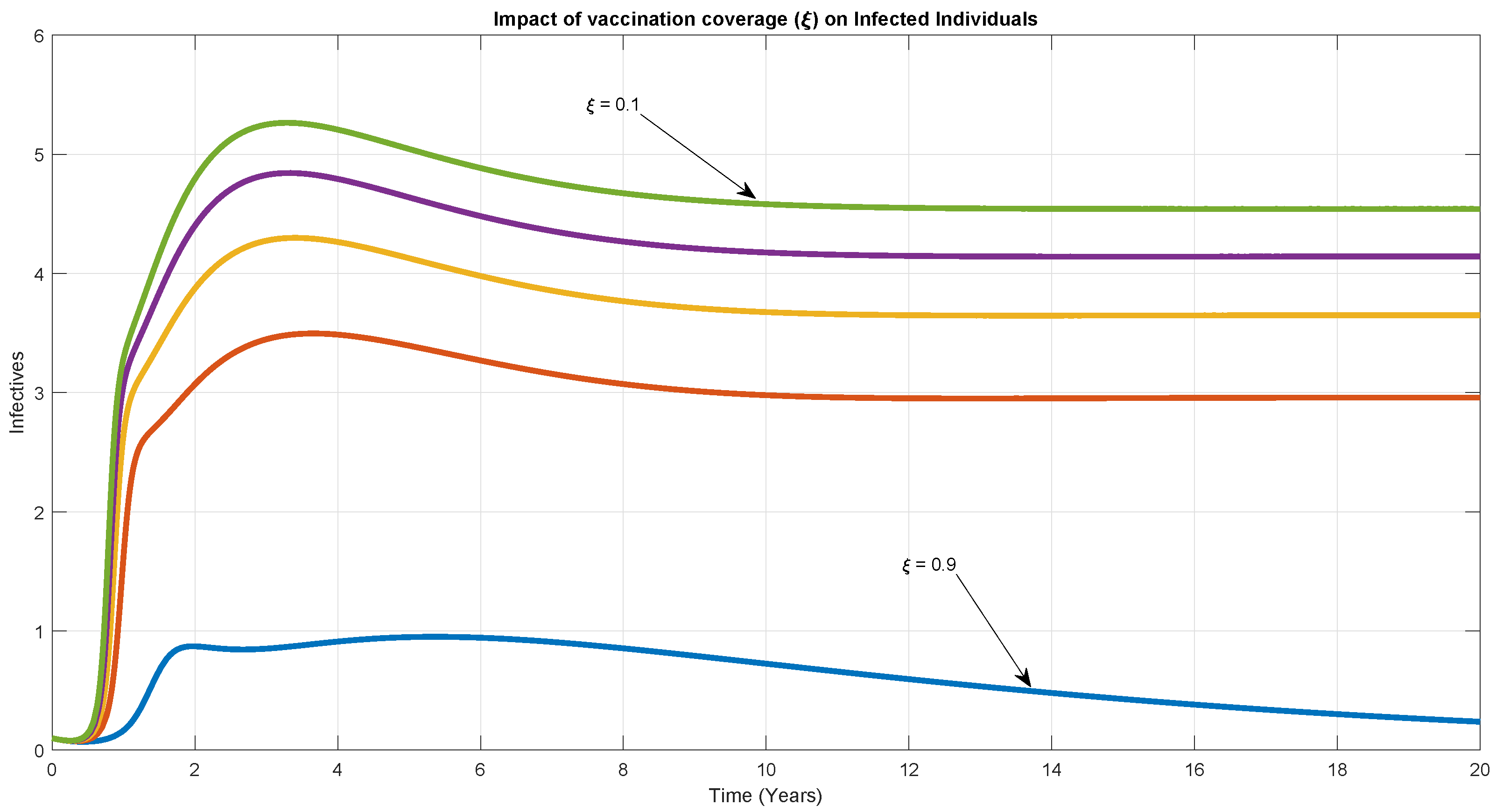
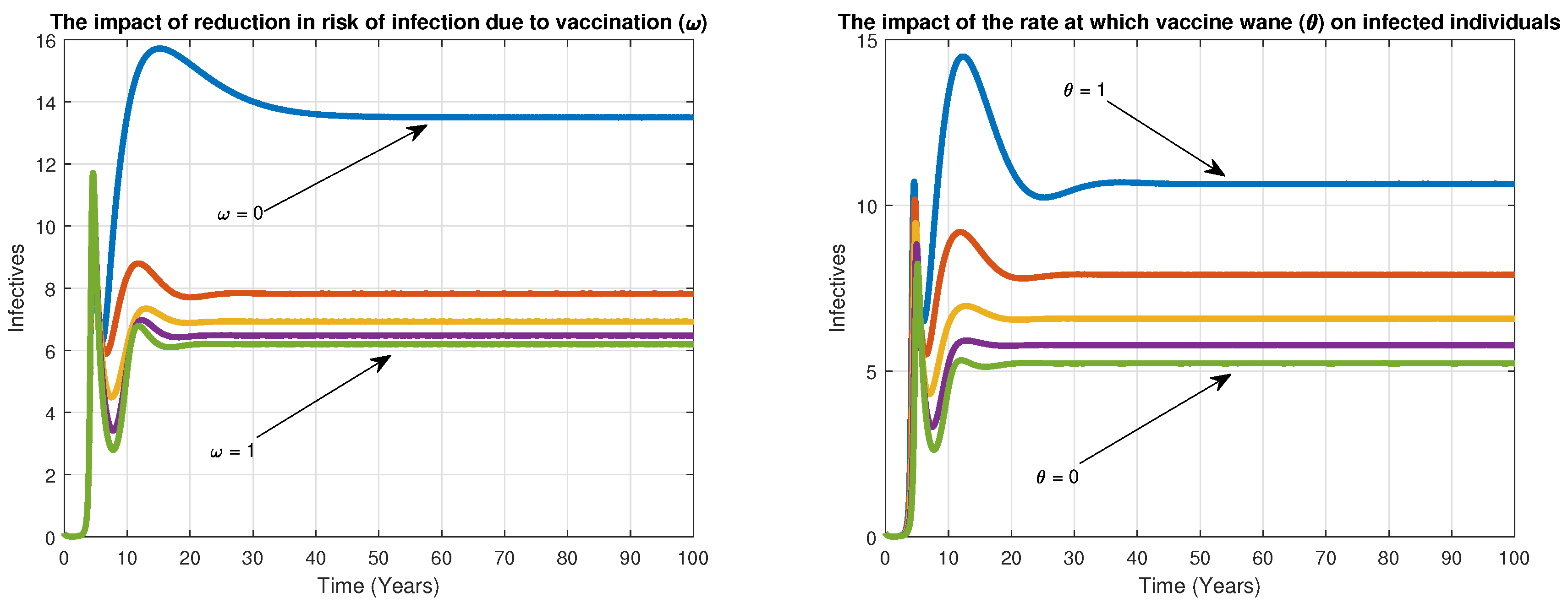
| Reduction in risk of infection due to vaccination | 0–1, 0.2, 0.90 | [74,75] | year | |
| The rate at which vaccine wanes | 0.067, 0.1 | [76,77,78,79] | year | |
| The rate at which susceptible individuals are vaccinated | 0, 0.1,0.98,0.95 | [39,40,80] | year | |
| Natural death rate | 0.15 | [21] | - | |
| Disease-induced death rate due to TB | 0.12 | [18,81] | year | |
| Transmission rate | variable | - | - | |
| Reinfection among the treated individuals | 0–1 | [34,82,83] | - | |
| Progression rate | 0.02 | [21] | year | |
| Recovery rate | 1.5–3.5 | [35] | year, day | |
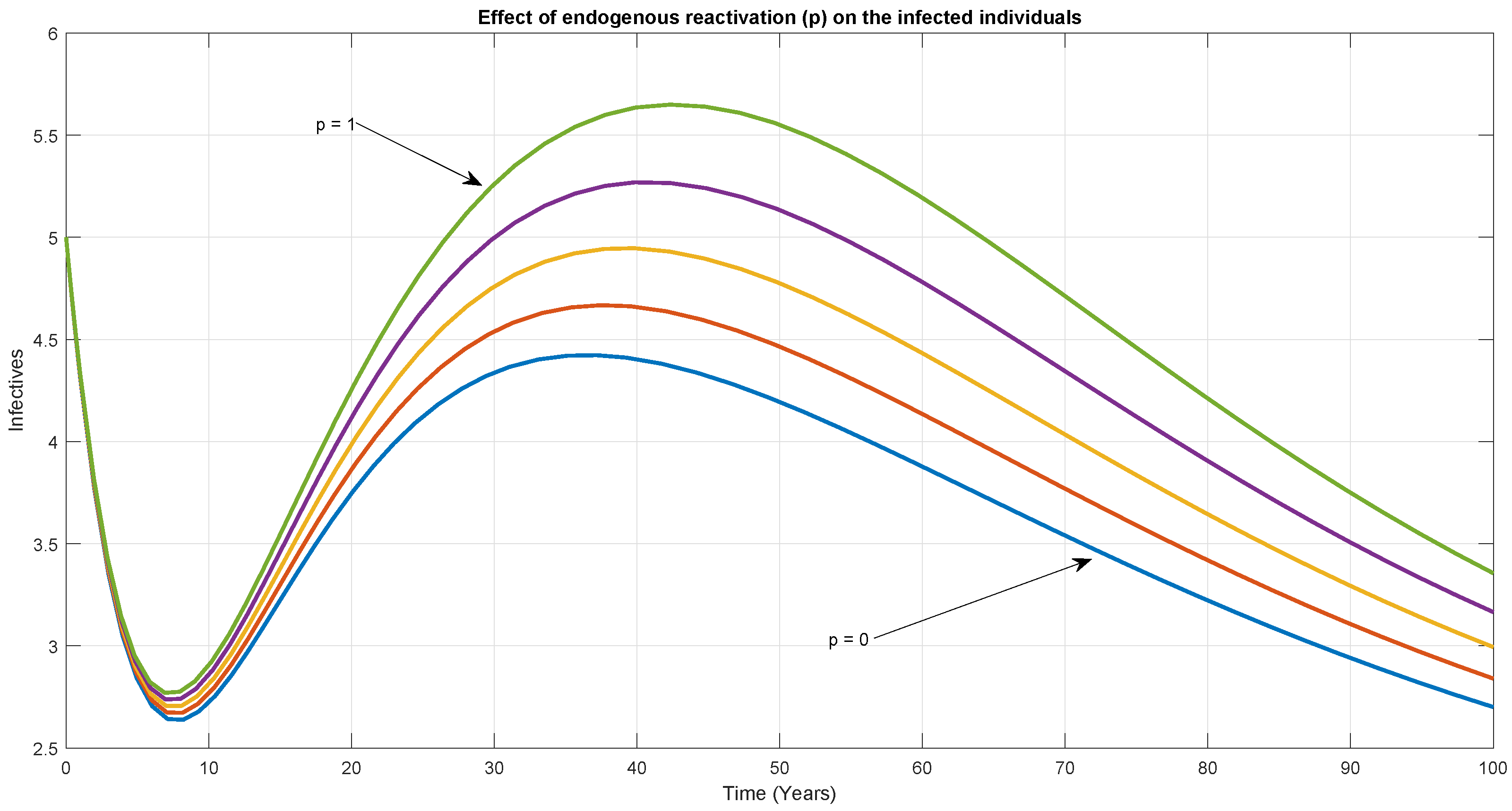
| p | Exogenous re-infection | 0–1 | [17,23,34,83] | - |
Publisher’s Note: MDPI stays neutral with regard to jurisdictional claims in published maps and institutional affiliations. |
© 2021 by the authors. Licensee MDPI, Basel, Switzerland. This article is an open access article distributed under the terms and conditions of the Creative Commons Attribution (CC BY) license (http://creativecommons.org/licenses/by/4.0/).
Share and Cite
Sulayman, F.; Abdullah, F.A.; Mohd, M.H. An SVEIRE Model of Tuberculosis to Assess the Effect of an Imperfect Vaccine and Other Exogenous Factors. Mathematics 2021, 9, 327. https://doi.org/10.3390/math9040327
Sulayman F, Abdullah FA, Mohd MH. An SVEIRE Model of Tuberculosis to Assess the Effect of an Imperfect Vaccine and Other Exogenous Factors. Mathematics. 2021; 9(4):327. https://doi.org/10.3390/math9040327
Chicago/Turabian StyleSulayman, Fatima, Farah Aini Abdullah, and Mohd Hafiz Mohd. 2021. "An SVEIRE Model of Tuberculosis to Assess the Effect of an Imperfect Vaccine and Other Exogenous Factors" Mathematics 9, no. 4: 327. https://doi.org/10.3390/math9040327
APA StyleSulayman, F., Abdullah, F. A., & Mohd, M. H. (2021). An SVEIRE Model of Tuberculosis to Assess the Effect of an Imperfect Vaccine and Other Exogenous Factors. Mathematics, 9(4), 327. https://doi.org/10.3390/math9040327