Article

Optimization of Energy Consumption in Chemical Production Based on Descriptive Analytics and Neural Network Modeling

by
Alexey I. Shinkevich
1,
Tatiana V. Malysheva
1,
Yulia V. Vertakova
2 and
Vladimir A. Plotnikov
3,*
1
Logistics and Management Department, Kazan National Research Technological University, 420015 Kazan, Russia
2
Kursk Branch, Financial University under the Government of the Russian Federation, 305016 Kursk, Russia
3
General Economic Theory and History of Economic Thought Department, St. Petersburg State University of Economics, 191023 St. Petersburg, Russia
*
Author to whom correspondence should be addressed.
Mathematics 2021, 9(4), 322; https://doi.org/10.3390/math9040322
Submission received: 5 January 2021 / Revised: 26 January 2021 / Accepted: 3 February 2021 / Published: 6 February 2021
(This article belongs to the Special Issue Mathematical and Instrumental Methods in the Digital Economy)

Abstract

:
Improving the energy efficiency of chemical industries and increasing their environmental friendliness requires an assessment of the parameters of consumption and losses of energy resources. The aim of the study is to develop and test a method for solving the problem of optimizing the use of energy resources in chemical production based on the methodology of descriptive statistics and training of neural networks. Research methods: graphic and tabular tools for descriptive data analysis to study the dynamics of the structure of energy carriers and determine possible reserves for reducing their consumption; correlation analysis with the construction of scatter diagrams to identify the dependences of the range of limit values of electricity consumption on the average rate of energy consumption; a method for training neural networks to predict the optimal values of energy consumption; methods of mathematical optimization and standardization. The authors analyzed the trends in the energy intensity of chemical industries with an assessment of the degree of transformation of the structure of the energy portfolio and possible reserves for reducing the specific weight of electrical and thermal energy; determined the dynamics of energy losses at Russian industrial enterprises; established the correlation dependence of the range of limiting values of power consumption on the average rate of power consumption; determined the optimal limiting limits of the norms for the loss of electrical energy by the example of rubbers of solution polymerization. The results of the study can be used in the development of software complexes for intelligent energy systems that allow tracking the dynamics of consumption and losses of energy resources. Using the results allows you to determine the optimal parameters of energy consumption and identify reserves for improving energy efficiency.

1. Introduction

For chemical industries, minimizing the negative impact on the environment caused by the use of fuel and electricity is a priority. Saving energy resources leads to a decrease in the load on the ecosystem and is one of the key objectives of the environmental policy. Energy Saving Programs are based on the principles of energy management, which are becoming increasingly popular in Russia and in other countries of the world. The use of the best available technologies and the achievements of energy management allows the enterprise management to build an efficient energy system in production with the lowest design and operating costs.
This research examines two interconnected topical areas—the energy component of the cost of production and the transformation of the structure of energy resources. The subject of the study is chemical industries. Chemical companies can make energy savings by applying energy management principles and methods. However, the use of energy management system tools will be most effective if they work in conjunction with an environmental management system that adheres to the principles of “green chemistry”.
According to the theory of “green chemistry” by Anastas and Warner [1], when planning synthesis, one should consider the economic and environmental consequences of the production of energy necessary for carrying out a chemical process and strive to minimize them. In this regard, it is important to conduct system monitoring and data analysis based on methods of descriptive analytics and statistical training in order to determine possible reserves for reducing the energy intensity of products, identifying the causes and normatively acceptable values of energy resource losses.
Numerous works of researchers are devoted to the issues of increasing the energy efficiency of industrial production in general and chemical–technological systems. The main directions of research in the field of green chemistry and sustainable consumption of energy resources are determined by the work of the following scientists: Chen et al. investigated the latest achievements of power engineering in the field of light chemistry [2]; Phan and Luscombe studied recent advances in environmentally friendly, sustainable synthesis of semiconductor polymers [3]; Delgado-Povedano and Luque de Castro evaluated the development of green analytical chemistry [4]; Liu et al. substantiated water-soluble, high-quality graphene as a green solution for efficient energy storage [5]; Mandal developed the theory of alternative energy sources for sustainable organic synthesis [6]; Wang and Feng deepened the knowledge of advanced materials for green chemistry and renewable energy [7]; Vertakova and Plotnikov proposed new technical energy-saving solutions based on waste processing [8].
Approaching environmental problems of energy conservation using mathematical tools is considered by a number of scientists: Meshalkin et al. presented an intelligent logical informational algorithm for choosing energy- and resource-saving chemical technologies [9]; Shang et al. summarized the characteristics of energy consumption and energy-saving strategies in the transition to energy-intensive machines of higher power [10]; Klemes and Varbanov substantiated the reduction of environmental pollution as a result of optimization of heat transfer [11]. Directions for improving the environmental friendliness of chemical production based on solutions in the field of introducing energy-saving organizational technologies are proposed in several other scientific works [12,13,14,15,16]. The use of evolutionary algorithms is possible in solving industry engineering problems: optimization of the maintenance process of power gas turbine plants to adjust the regulator parameters in order to reduce equipment downtime and reduce the level of energy consumption; optimization of the process of cyclic injection of coolants into the oil reservoir; minimization of energy expended during steam generation and reduction of waste-water at a production well, etc.
The importance of solving the problems of reducing energy consumption in various industries has caused the need to use optimization methods. To solve these problems, classical methods of mathematical optimization are widely used [17]. In recent years, new optimization methods have been developed, such as new crossover methods for real coded genetic algorithms that improve the quality of the solution, the data transfer rate and the determination of the optimal solution [18]; an optimization algorithm based on Mendel’s evolutionary theory [19]; an evolutionary optimization method based on the biological evolution of plants [20]; a genetic algorithm based on the technique of extended selection and logarithmic mutations [21]; etc. Variants of genetic algorithms, particle swarm algorithms and Mendel’s evolutionary theory are also presented in the book by Simon [22] and in the works of Chih-Ta and Ming-Feng [23], Haiping et al. [24], Janet et al. [25], Salman and Khan [26], Sidahmed [27], etc.
Economic and technological processes proceed based on the principle of causality [28]. This determined their active use for their analysis and modeling of Artificial Neural Networks [29,30,31,32,33,34,35]. The main advantage of using neural networks is their ability to self-learn, i.e., to form new knowledge about the modeled process. This property allows using a neural network to solve complex problems that do not have an explicit solution. In addition, the positive effects of using neural networks are: solving problems with unknown patterns between the input and output data; resistance to noise in the input data; adaptation to environmental changes, the ability to use neural networks in a non-stationary environment due to automatic retraining (adaptation); high performance due to parallel processing of information.
The high complexity and uncertainty of energy consumption processes make it preferable to use neural networks to study them [36,37,38,39,40]. In order to expand the mathematical tools for studying the energy efficiency of chemical industries, Jin et al. developed approaches to assessing the effectiveness of resource-saving projects based on a backpropagation neural network [41]; Xiang et al. proposed an algorithm for learning a multilayer neural network based on photonic spike timing dependent plasticity [42]; Menghi et al. systematized methods and tools for energy assessment [43]; Geng et al. assessed the energy saving of complex petrochemical industries based on complex clustering of the DEA affinity distribution [44]; Hamedi and Mokhtar applied multivariate linear regression and multilayer perceptronic artificial neural networks to build a baseline for energy consumption in a low-density polyethylene plant [45]; Shinkevich et al. showed the advantage of the network model of the value chain for analyzing the resource intensity of production [46]; Rajskaya et al. substantiated the expediency of a differentiated approach to assessing the level of innovative development of production resource-saving systems [47].
However, despite the presence of significant theoretical and methodological material and analytical data, there is a lack of research to solve the problems of efficient energy consumption by chemical industries. The lack of completeness of scientific and practical knowledge and solutions in the field under study does not allow us to objectively analyze the management processes of chemical and technological systems or to consider the specifics of production from the standpoint of optimal energy consumption.
One of the important issues that arise during energy analysis and monitoring of the implementation of energy-saving measures within the energy management system is the assessment of energy efficiency. This assessment is carried out on a few quantitative characteristics. At the same time, almost all Russian companies implementing energy efficiency programs aim to reduce the share of energy consumption in the cost of production. The urgency of this problem is high. The share of costs for electric and thermal energy in the cost of chemical products in Russia reaches an average of 13%. In comparison, in high-energy metallurgy, this figure is 9%, which confirms the relevance of energy conservation in the chemical industry. For many types of fuel and energy, the cost of resources in Russia is lower than, for example, in Western Europe. However, this does not always give Russian chemical companies an advantage due to the inefficient use of energy resources.

2. Materials and Methods

2.1. Basic Research Methods

As the main research methods, the article uses graphic and tabular tools for descriptive data analysis to study the dynamics of the structure of energy consumption and determine possible reserves for reducing its consumption. To determine the measure of the spread of the values of the specific weight of the resource relative to its average value, the variance of the values (D), which make up the data array on the structure of energy resources, was calculated using the formula:
D = M(x − M(x)2), M = (Σ x) / n,
where x is the value of the specific weight of the energy resource, M is the average value of the specific weight of the energy resource in the energy portfolio, n is the number of periods.
The standard deviation of the population of data on the structure of energy resources (S), calculated as a percentage and more accessible for data interpretation, is defined as the positive square root of the variance of the population:
S = (M(x − M(x)2))0.5, M = (Σ x) / n.
To determine the possible reserve for reducing the share of energy in the consumption structure, the calculation of the interquartile distribution, namely the first lower or 0.25 quartile and the third upper or 0.75 quartile, is proposed. The reserve for reducing the specific weight of the resource (R) is defined as the difference between the actual value and the value of the lower-order quartile according to the formula:
Ri = Fin − Qin = Fin − xQ1 + iQ1 × (Σfi / 4 − sQi−1) / fQi,
where F is the actual value of the specific weight of the resource for the period, Q1 is the lower-order quartile, ∑fi is the sum of the frequencies of the series, n is the period, i is the type of energy resource.
To predict the maximum possible values of energy consumption, a statistical learning method is proposed—a method for training neural networks based on a regression predictive model. In contrast to traditional computing systems, optimization of parameters using neural networks allows solving problems with unknown patterns of development of the situation, an unstable relationship between input and output data. In the chemical industry, in relation to which the research was carried out, the probability of emergency situations, unstable operation of technological lines can determine the non-stationarity of energy consumption. This requires optimization systems to be adaptive for robust modeling. Neural networks have the ability to adapt to changes in external parameters and uncertainty of input data. Therefore, this method was chosen for modeling.
In this study, we used a type of multilayer neural network MLP, where one backpropagation algorithm trains all layers. Multilayer perceptrons MLP can be interpreted as an input–output model in which weights and constraints on value bias are free parameters of the model. Activation functions for hidden and output neurons can be both smoothed (logistic σ ( t ) = 1 1 + e t , hyperbolic t h ( t ) = e t e t e t + t t ) and the identity g(t) = t and exponent exp ( t ) = e t .
The iterative method of numerical optimization BFGS (Broyden–Fletcher–Goldfarb–Shanno algorithm) was used as a network learning algorithm, aimed in this case at finding the local minimum energy consumption at the upper limit of the range. The analysis methods were implemented using the Microsoft Office Excel software from the MS Office package and the STATISTICA software package.

2.2. Information Basis of the Research

The main informational study of the structure of fuel and energy resources in the chemical industry and forecasting the optimal consumption of energy resources is the dynamics of the energy component of the cost of production (Table 1) and the structure of fuel and energy resources in the production of chemicals from 2012 to 2019 (8 years) (Table 2). The calculations used data from the Federal State Statistics Service (Russia), as well as data from Russian chemical enterprises.
An important parameter of energy efficiency in industry is the energy component of the production cost or the share of fuel and energy resources in the production cost (Table 1). In 2019, according to the Federal State Statistics Service, in the production of chemicals and chemical products, the share of all fuel and energy resources was 13.25%. At the same time, the share of thermal energy in the cost of production was 6.13%, electric energy was 4.93% and water for technical needs was 0.18%. The share of fuel in the cost of production (gas, fuel oil, coal, gasoline, diesel fuel) amounted to 2.01% in total.
The averaged structure of fuel and energy resources in the production of chemicals and chemical products according to the Federal State Statistics Service included, in 2019, 37.2% of electric energy and 46.3% of thermal energy (Table 2). Traditionally, 1–2% falls on water. Among the types of fuel, combustible natural gas (12.7%) occupies a predominant position, and the other types account for no more than 2%. The movement of the structure of fuel and energy resources in dynamics for 2012–2019 for certain items is quite significant. This may be due to the change in the cost of energy resources, the transformation of the product range, the introduction of new technological equipment, as well as the effect of the implementation of corporate energy-saving programs.
Thus, to increase the competitiveness of Russian products, the priority direction of the energy conservation policy for the production of chemicals and chemical products should be to reduce the share of fuel and energy resources in the cost of production. Modernization of the energy management system at the enterprises of the industry will make it possible to implement a complex of interrelated elements in the form of organizational measures, technical means and software, and methodological support in the direction of energy-saving and sustainable consumption of energy resources.

3. Results

3.1. Descriptive Statistics of Changes in the Structure of Fuel and Energy Resources in the Production of Chemicals and Chemical Products

Analysis of the database on the energy component of the cost of chemical products showed the importance of studying the dynamics of the structure of fuel and energy resources used by enterprises in this industry for production. Complex chemical–technological systems have more complex reserves of energy conservation and have additional effects from the optimization of energy flows. At the enterprise level, the possibilities for modernization and development of energy systems are not limited to technical measures but are complemented by solutions and analytical methods for identifying reserves, as well as methods for improving management systems. Moreover, the introduction of technical tools is not exhaustive. The power supply of the chemical–technological system constantly requires adjustment due to the development of technical progress.
The energy management system assumes the organization of system monitoring and analysis, where the energy component of the production cost is considered among the energy efficiency indicators. Monitoring and energy analysis are necessary in order to provide information support for the continuous process of improving the results of the use of energy resources. The database on the structure of energy resources used in the production of chemical products (Table 2) shows a significant variation in the dynamics of fuel and energy.
To simplify the interpretation of the results of graphical data analysis, Table 3 shows descriptive statistics of the structure of fuel and energy resources in the production of chemicals and chemical products in 2012–2019.
A given space with random values of the consumption of fuel and energy resources X with distribution PX can be described by the distribution function:
Fx: R → [0,100].
The distribution function is given by the formula:
FX (x) = P (X ≤ x) = PX [(− ∞, x]).
thus, the distribution function of the specific gravity of resource consumption X is the function F(x), the value of which at the point x is equal to the probability of the event {X ≤ x}, consisting only of the space of elementary events ω, expressed as X (ω) ≤ x.
When evaluating the range of variables, the formulas for the lower boundary of the whisker X1 and the upper boundary of the whisker X2 are:
X1 = Q1 − k (Q3 − Q1),
X2 = Q3 + k (Q3 − Q1),
where Q1 is the first quartile (lower-order quartile), Q3 is the third quartile, k is a coefficient of 1.5.
Statistical parameters make it possible to generalize the primary results, present the distribution of their frequencies and identify the central trends in the change in the capacity of the energy portfolio relative to a resource. The reserve for reducing the specific weight of the resource is defined as the difference between the actual value of 2019 and the value of the lower order quartile Q1.
Analysis of the change in the share of electric energy in the energy portfolio of chemical industries produced some results. A positive trend is the greater number of cases with the share of electricity in the volume of resources of 31–33%, included in the quartile of the lower or first order (Q1 = 32.13), which can be visually observed on the swing diagram. The variance of the analyzed resource relative to other resources has an average value D = 10.6. Accordingly, the standard deviation of the dynamic range of electrical energy S = 3.2%. The asymmetry coefficient A = 0.212 indicates a greater deviation of the values in the positive direction, i.e., the tendency for the predominance of values above the average value (M = 34.99%) remains. A negative kurtosis coefficient characterizes the absence of peaked data distribution. In general, the analysis shows a low spread in the share of electricity in the energy portfolio and a high frequency of minimum possible values, which is a positive point and shows the reserve for a decrease in the indicator at 5.07 percentage points.
An analysis of the change in the share of thermal energy is characterized by the largest magnitude of the swing (D = 27.71) and a deviation from the average value of 5.2%. At the same time, according to the coefficient of asymmetry (A = −0.108), high values of the specific weight of thermal energy, equal to 53–55%, prevail in the dynamic series. The distribution of the indicator values in dynamics is flat-topped and has no peak values (E = −2.418). The analysis of descriptive statistics shows the instability of the share of thermal energy in the total volume of energy resources and the predominance of high values of the indicator in the sample. In this case, the possible reserve for the decrease in the indicator will be less significant and amount to 0.95 percentage points.
An analysis of the change in the share of fuel (combustible gas, fuel oil, coal, gasoline, diesel fuel) in the energy portfolio of chemical industries shows the predominance in the dynamics of high values of the specific gravity of fuel (15–16%). The variance of the analyzed resource has a low value (D = 4.71). Accordingly, the standard deviation of the dynamic range of the fuel is insignificant (S = 2.2%). In general, the analysis shows a stable dynamic of the share of fuel resources with a bias of data towards higher values. With the indicator level in 2019 of 15.15%, the possible reserve for its reduction can be estimated at 3.4 percentage points.
The dynamic series of the share of water for technical needs in the energy profile of chemical industries shows a relatively even distribution of values with the established dynamics of the indicator of 1.7–1.4% in 2017–2019. Accordingly, there is a minimum variance (D = 0.18) and a series deviation (S = 0.42%). For this energy resource, the possible reserve for reducing the specific weight of water in the volume of resources is not more than 0.04 percentage points.
To determine the possible reserve for reducing the share of energy in the structure of resources, the interquartile distribution was calculated, namely the first lower or 0.25 quartile and the third upper 0.75 quartile. The reserve for reducing the specific weight of the resource (R) is defined as the difference between the actual value of 2019 and the value of the lower-order quartile by Formula 3.
Thus, the analysis showed the largest possible reserve for reducing the specific weight of electrical energy with existing production technologies. Given the high cost of this resource, the reduction in the cost of production due to energy conservation can be tangible. At the end of 2019, the share of electric energy in the cost of chemical production amounted to 4.93%. At the same time, the minimum value for the study period was noted at 4.5%. At the same time, thermal energy cannot be excluded from the list of priorities, the share of which in the cost of production in 2019 reached 6.13%.

3.2. Neural Network Models for Predicting Optimal Energy Consumption at the Upper Limit of the Range of Values

The method of statistical training of neural networks predicted the maximum possible values of energy consumption. As the initial data, the quarterly dynamics of the structure of energy resources consumption in the production of chemicals for 32 time periods was used (quarterly data for 2012–2019). The learning algorithm is based on a regression predictive model, where the objective function is:
C m a x o p t = f ( C m i n 1 n ¯ , C m e d 1 n ¯ , S n , D n ) ,
where C m a x o p t is the optimal value of energy consumption at the upper limit of the range (maximum value), C m i n 1 n ¯ is the value of energy consumption at the lower limit of the range (minimum value) for the study period, C m e d 1 n ¯ is the average value of energy consumption for the study period, Sn is the standard deviation of the value in the variational series, Dn is the variance of the data series, n is the number of periods in the data series.
The categorical input variable is expressed in terms of C m e d 1 n ¯ , and the continuous input variable is expressed as C m i n 1 n ¯ . A linear regression relationship is determined between the continuous target variable and the input variables. Accordingly, the continuous target variable is the most optimal energy consumption value at the upper limit of the C m a x o p t range. Since the structure of the energy portfolio is limited by a certain set of energy resources with limiting values of consumption according to chemical technology and the level of reliability (95.0%) of the parameters of the time series, the following conditions must be satisfied:
{ C m a x o p t E 1 9 = 100 42.00 C m a x o p t E 1 56.00 31.00 C m a x o p t E 2 41.00 1.00 C m a x o p t E 3 2.50 8.00 C m a x o p t E 4 14.00 0.40 C m a x o p t E 5 1.80 0.10 C m a x o p t E 6 0.21 0.01 C m a x o p t E 7 0.20 0.20 C m a x o p t E 8 0.70 0.30 C m a x o p t E 9 0.80
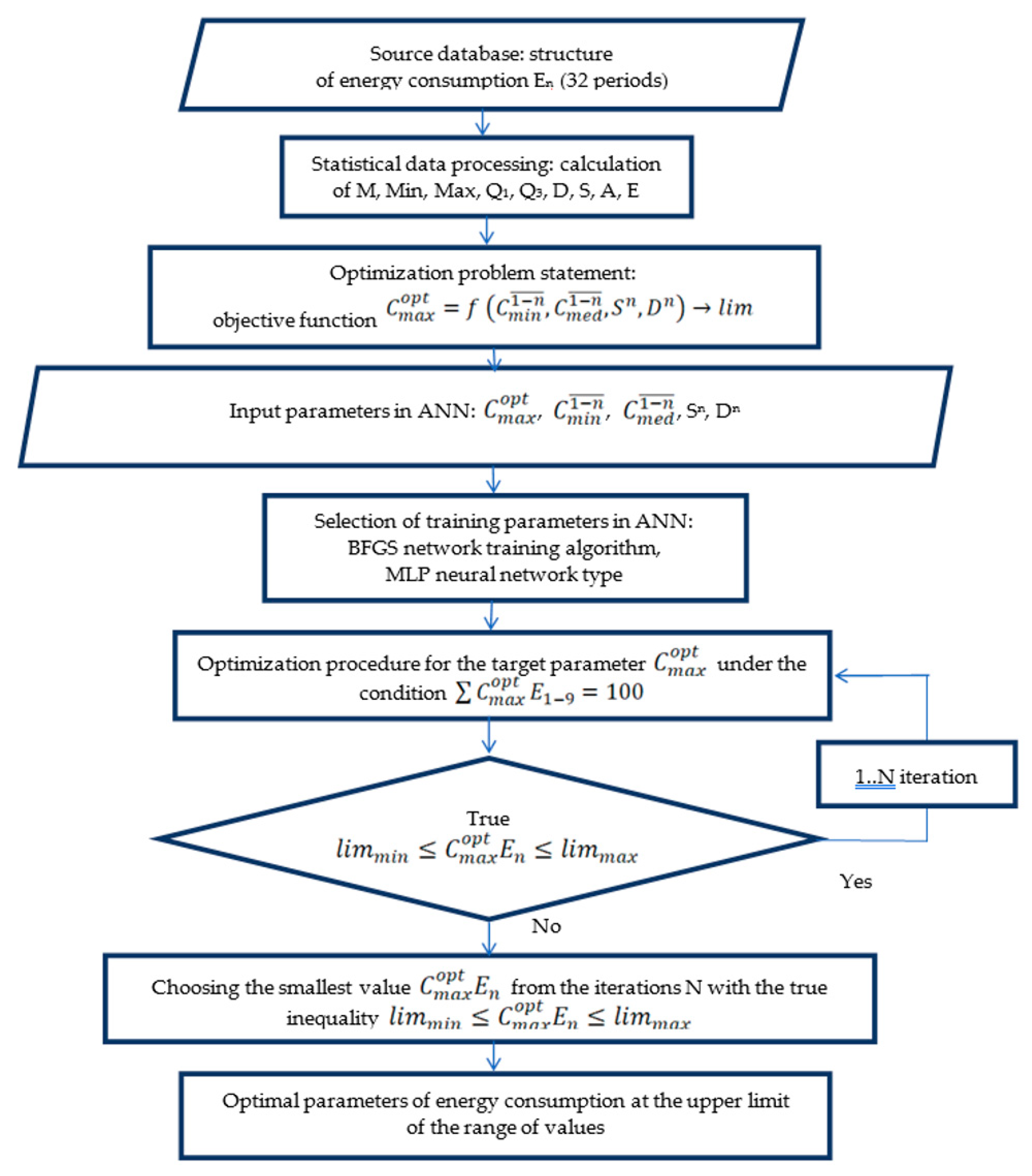
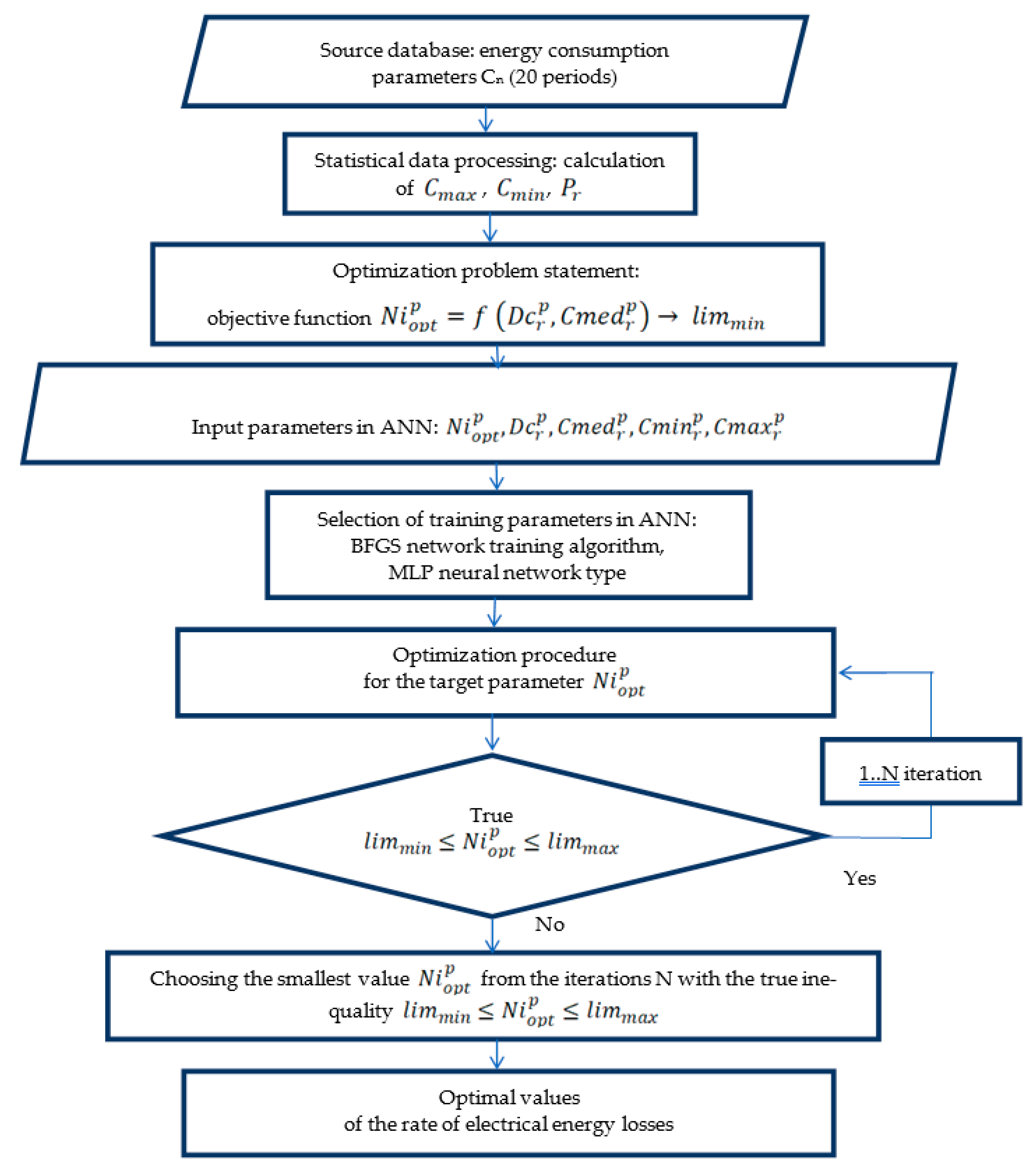
A block diagram of finding the optimal energy consumption by the method of training neural networks is shown in Figure 1. The procedure includes five main stages:
  • Step 1. Primary statistical processing of an array of data on the structure of energy resources consumption with obtaining the necessary parameters for training neural networks.
  • Step 2. Statement of the optimization problem—determination of the minimum possible value of the objective function—the parameter of energy resource consumption at the upper limit of the range, considering the restrictions.
  • Step 3. Selection of neural network training parameters: BFGS iterative numerical optimization method as a network training algorithm and MLP type of neural network.
  • Step 4. The procedure for optimizing the target parameter under the condition of maintaining the integrity of the energy portfolio structure C m a x o p t E 1 9 = 100 . The algorithm is executed if the inequalities under the constraints l i m m i n C m a x o p t E n l i m m a x are true.
  • Step 5. Determination of the target optimal parameter by choosing the smallest value C m a x o p t E n from the variants of training cycles—iterations N with the true inequality l i m m i n C m a x o p t E n l i m m a x .
Input parameters were set at 20 networks for training and 5 networks for saving. The results of the neural network models are presented in Table 4.
According to the resulting architecture, each of the saved MLP networks has five input variables and one variable at the output C m a x o p t according to the objective function, and the number of hidden neurons varies from 3 to 8. The highest performance or specific weight of correct classification on the training and control samples is possessed by 3–5 neural networks (96–99%). The iterative method of numerical optimization BFGS (Broyden—Fletcher—Goldfarb—Shanno algorithm) was used as a network learning algorithm, aimed in this case at finding the local maximum consumption of energy resources. The optimal value at the highest level of control performance (network No. 4) was found in 24 training cycles.
In the study, the object of statistical training is the structure of energy resources of chemical industries, which includes nine components: thermal energy (E1), electrical energy (E2), water (E3), natural combustible gas (E4), diesel fuel (E5), fuel oil (E6), coal (E7), gasoline (E8) and other fuels (E9). The specific weight of each resource Ei in the general structure of energy resources is as follows:
E i = C i × 100 1 m C i , m = ( 1 , 9 ¯ ) .
Thus, as a result of training the neural network (network No. 4 MLP 5-3-1), the optimal values of energy consumption were obtained at the upper limit of the range of values (maximum values), which, as can be seen, in most cases do not have a significant deviation from the objective function (Table 5). During the statistical processing of the data, the resources of natural combustible gas (E4) and gasoline (E8) were removed from the sample due to the presence of values with a high level of variation.
The optimal structure of the energy resources of chemical industries contains E1 = 55.48%, E2 = 39.59%, E3 = 2.35%, E5 = 1.71%, E6 = 0.21%, E7 = 0.19%, E9 = 0.48%. Undoubtedly, the absence of the primary specified components E4 and E8 in the structure of energy resources requires additional analysis with the participation of engineers in the field of chemical technology.
The use of the neural network training method made it possible to simulate the optimal structure of energy resources of chemical production, which is an important component of the strategy of resource conservation and increases the competitiveness of the Russian industry. In addition, a significant parameter of resource efficiency of production is the loss of fuel and energy resources. Losses of energy resources in distribution networks are inevitable; therefore, it is important that they do not exceed a reasonable level. An increase in the rates of technological consumption of fuel and energy resources indicates the problems that have arisen, and to eliminate them it is necessary to identify the causes of inappropriate costs and determine the directions of their reduction.

3.3. Graphical Statistics of the Dynamics and Interdependence of Losses of Electrical and Thermal Energy in the Distribution Networks of Industrial Production

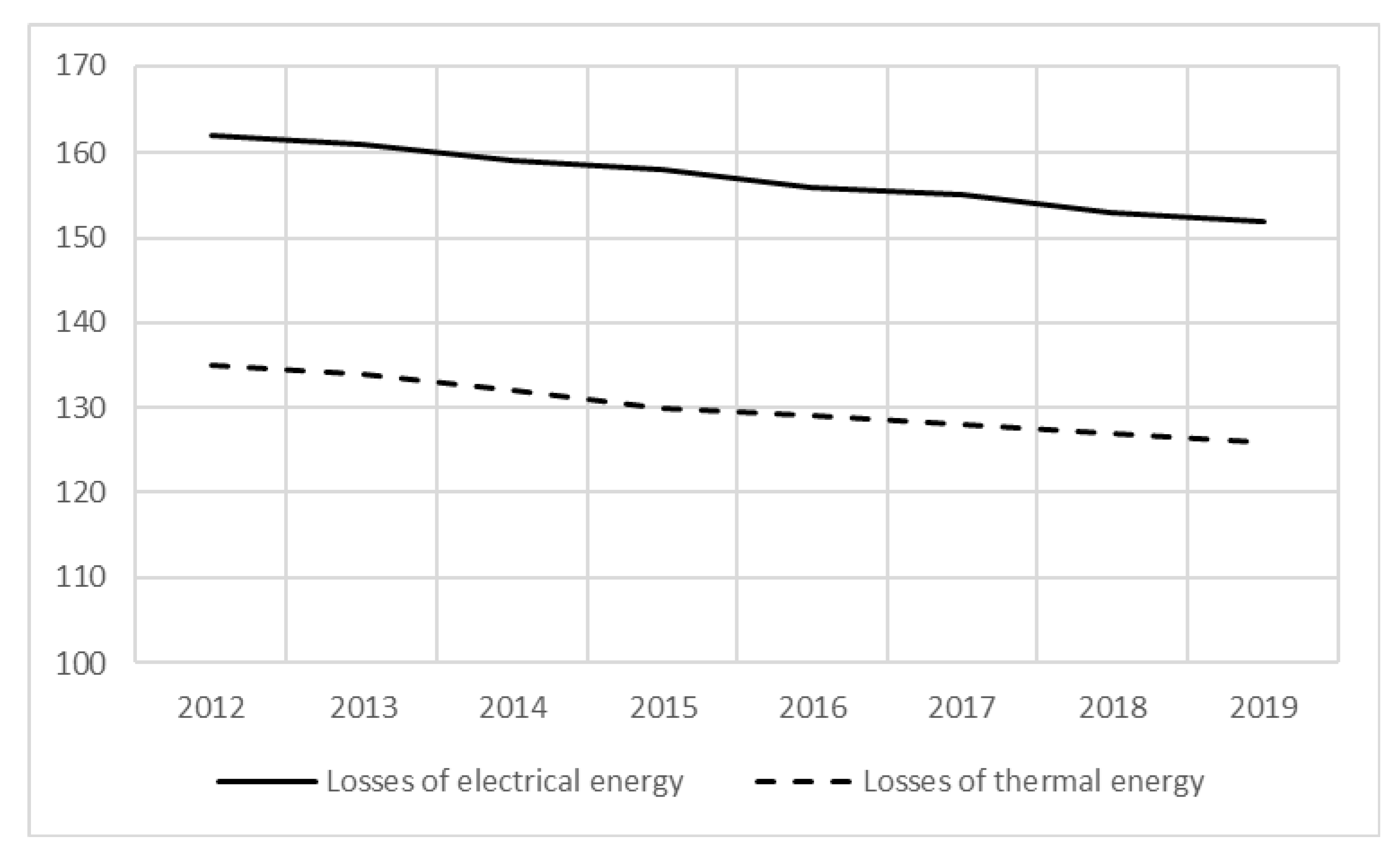
For the studied years 2012–2019, there is a positive trend in reducing the amount of energy losses, both in electrical (reduction index in 2012–2019—93.8%) and thermal energy (reduction index in 2012–2019—93.3%) (Figure 2). However, the amount of electricity losses of 15.2% of the total volume of transmitted energy remains relatively high in Russia. In comparison, in industrially developed countries it is as follows: Germany—7.6%, Finland—6.7%, USA—6.5%, Canada—6.3%, Japan—5%.
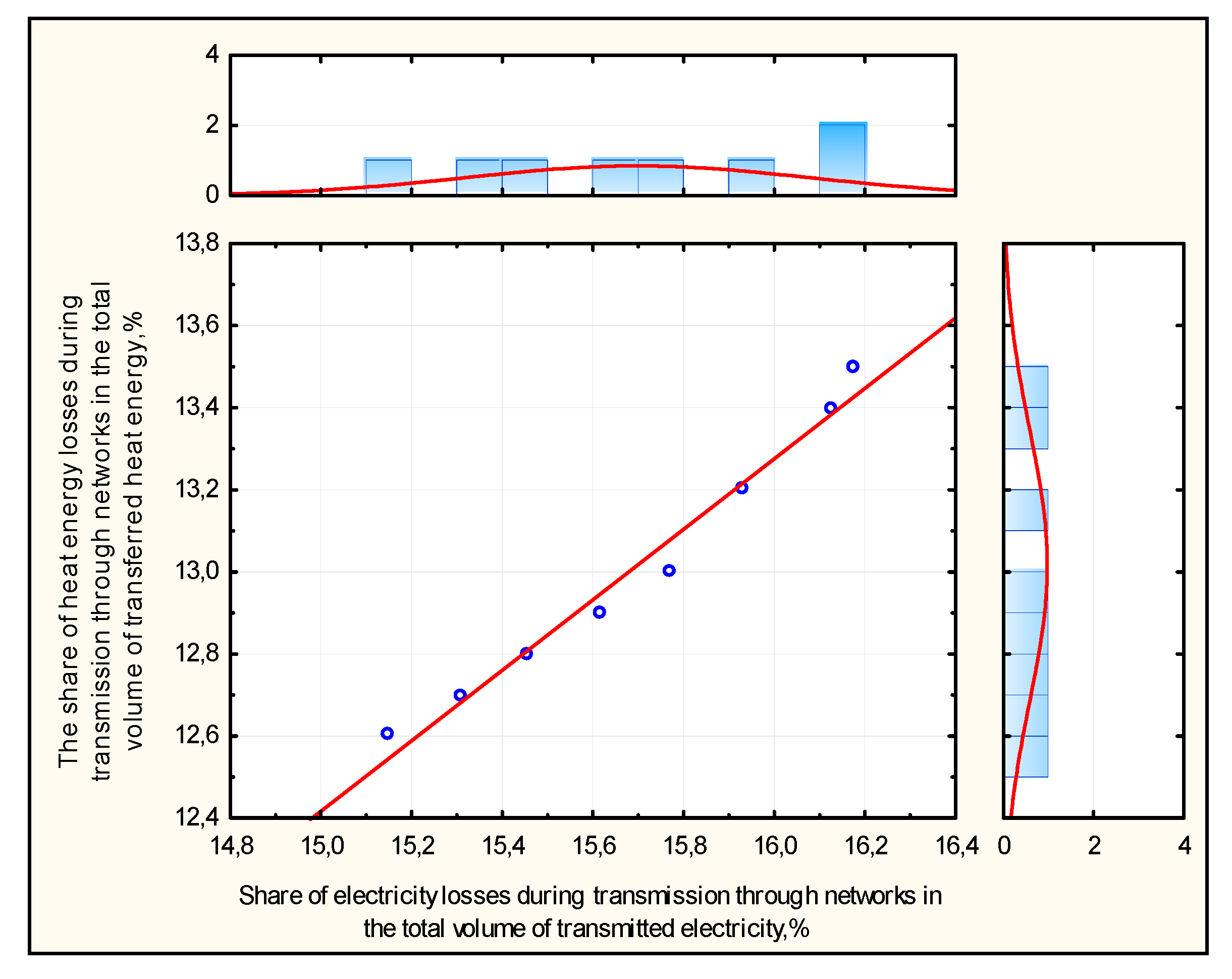
Figure 3 shows a scatter diagram that visualizes the relationship between losses of electrical and thermal energy in distribution networks. The equation of the linear trend of the obtained dependence on the scatter diagram has the form Y = −0.4688 + 0.859X. Correlation coefficient of heat and electric energy losses Kor = 0.98. This indicates a close relationship between the parameters. A stable reduction in the amount of energy losses in distribution networks is probably not a random phenomenon but is due to purposeful management actions of executive authorities and enterprise management [48].
Russian chemical producers have indicators of the consumption of fuel and energy resources. These indicators are published in the industry’s best available technology reference books. These guides give the minimum and maximum possible consumption of energy resources for specific types of products. The range between the minimum and maximum values of resource consumption is justified by existing traditional and innovative production technologies, the degree of deterioration of energy networks and the specificity of the chemical technology of the product.
For example, the Russian polymer manufacturer PJSC “Nizhnekamskneftekhim” produces five grades of solution polymerized rubbers with a total volume of about 1.9 million tons per year. Each type of rubber has a standardized minimum and maximum value of the specific consumption of energy resources. The amount of excess of the max value over the min value of the resource consumption (r) is calculated by the formula:
Pr = Cmax(r) / Cmin(r) × 100.
The calculation results are shown in Table 6. The value of the excess of the max flow rate over the min value differs significantly. Synthetic butadiene-styrene rubber DSSK-2565F and synthetic cis-butadiene lithium rubber SKD-L have the highest specific energy consumption, for which the production of one ton, respectively, requires 667–693 kWh and 750–790 kWh of electric energy and 6.1–8.3 Gcal and 6.5–6.9 Gcal of thermal energy. As can be seen, for these types of rubber, there is a smaller corridor between the limiting values of resource consumption: the excess of min over max Pr = 103.9% and Pr = 105.3% for electrical energy. For thermal energy, the range of limit values is somewhat wider than for electrical energy. The reason for this phenomenon is the technological features of heat exchange processes and equipment.
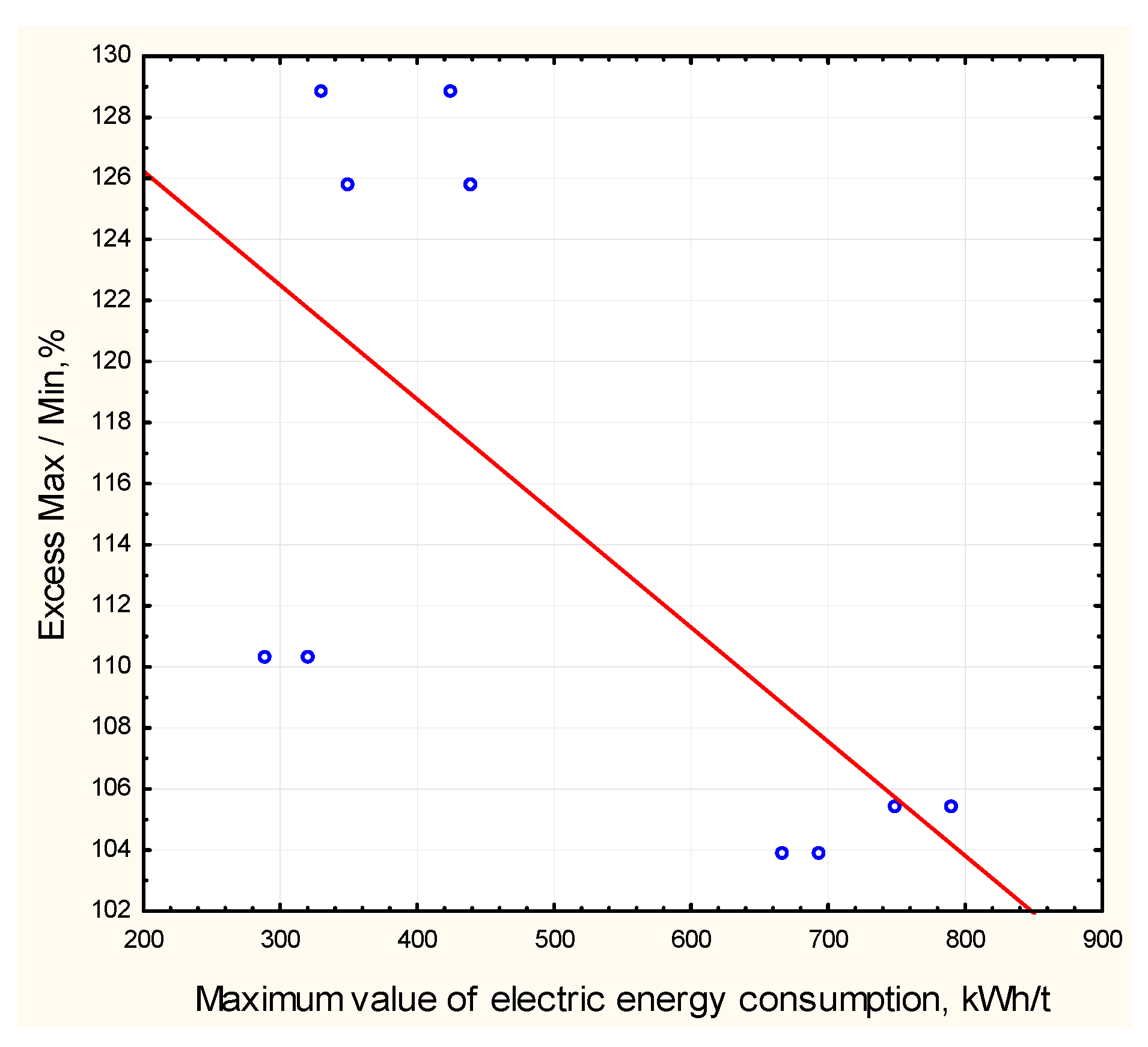
The range of limit values of specific energy consumption as a percentage of Dcr is expressed mathematically through the excess of the max value over the min value: Dcr = Pr—100. The dependence of the range of limit values of specific energy consumption on the average consumption rate is confirmed in the scatter diagrams. Figure 4 shows an absolute inverse relationship between the values of the electrical capacity of rubber and the range of the min–max values corridor (correlation coefficient Kor = −0.77). Therefore, it can be assumed that in the production of high-power products, the rate of loss of electrical energy should be significantly lower. Attention should be paid to technical losses of electricity due to physical processes in electrical equipment, avoidance of idle time and downtime of high-power installations.
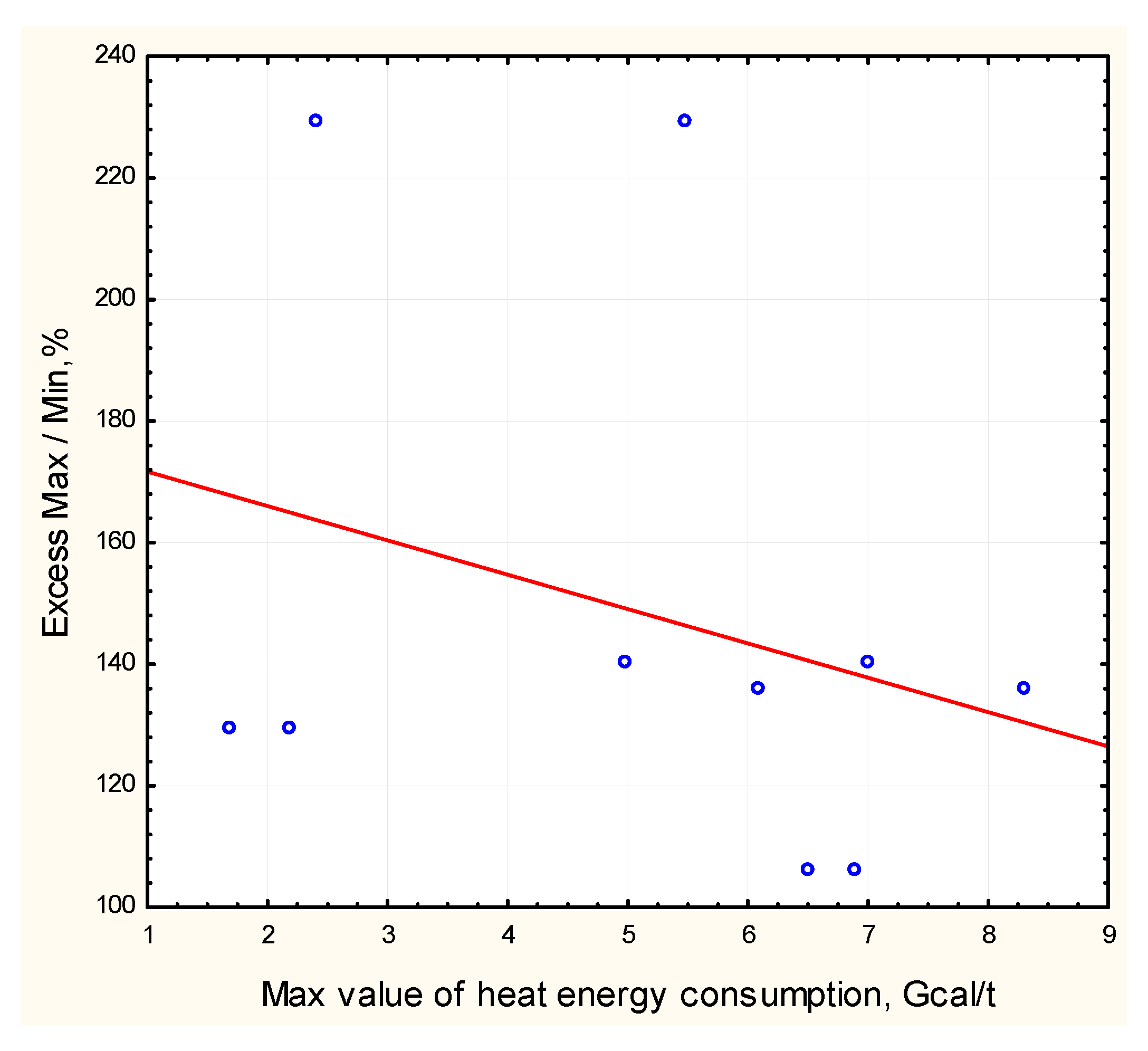
The dependence of the range of limiting values of the specific consumption of heat energy on the average consumption rate is weakly negative, with small tightness of connection (Kor = −0.35) (Figure 5). The lower correlation of the parameters is due to the use of secondary heat resources in sufficiently large volumes due to the integration of cold and hot flows in chemical processes. It should also be noted that in addition to purchasing heat energy on the market, enterprises can produce it independently, spending electric energy on it. Nevertheless, we consider it expedient to use the criterion of the average specific resource consumption to produce products when calculating the rates of heat loss.

3.4. Development of Optimal Values of the Rate of Losses of Electrical Energy for Rubbers of Solution Polymerization Based on Training a Neural Network

To determine the rate of losses of electrical energy Ni in the production of rubbers of solution polymerization, depending on the range of limit values of energy consumption proposed in the handbook on the best available technologies, a regression method was used for training neural networks. The objective function is:
N i o p t p = f ( D c r p , C m e d r p ) l i m m i n ,
C m e d r p = ( C m i n r p , C m a x r p ) 2 ,
where N i o p t p is the optimal value of the rate of electrical energy losses by polymer, D c r p is the range of limit values of electricity consumption by polymer, C m e d r p is the average value of electricity consumption by polymer, C m i n r p is the minimum value of electricity consumption for polymer, C m a x r p is the maximum value of electricity consumption for polymer, p is polymer (solution polymerization rubber).
The optimization problem is to find the minimum possible value of the rate of electrical energy losses for the polymer (solution polymerization rubber), considering the established restrictions. The limits, according to the proposed approach, are determined based on the minimum and maximum values of electricity consumption for polymer in accordance with the Standard for Best Available Techniques [49]:
{ 0.08 N i o p t 1 0.12 0.08 N i o p t 2 0.12 0.10 N i o p t 3 0.15 0.10 N i o p t 4 0.15 0.05 N i o p t 5 0.09
The block diagram of finding the optimal energy consumption by the method of training neural networks is shown in Figure 6. The sequence of operations is according to the block diagram for determining the optimal energy consumption (see Figure 1).
As in the first case of training the network, here a type of multilayer neural network MLP is used, containing an input layer, an output layer and one hidden layer. The categorical input variable is expressed in terms of the polymer energy consumption rate converted to a text variable based on C m e d r p , two continuous input variables are represented as C m i n r p and C m a x r p . Accordingly, the continuous target variable is the optimal value of the rate of electrical energy losses for the polymer N i o p t p .
As a network learning algorithm, the BFGS numerical optimization method was also used to calculate the inverse Hessian based on changes in gradient values and changes in weights. The gradient vector of the error function is computed using the usual backpropagation procedure. The results of the neural network models are presented in Table 7.
All five neural networks have a high proportion of correct classification in the training and control samples. The highest training performance is observed in the second neural network MLP 5-9-1, representing five input variables, one variable at the output N i o p t p according to the objective function and nine hidden neurons. At the same time, the optimal value at the highest level of control performance was found in 32 training steps.
As a result of network training, synthetic cis-isoprene rubber SKI-3 was removed from the sample. The optimal values of the rate of electrical energy losses for the four types of solution polymerization rubbers in percentage are presented in Table 8.
Thus, as a result of training the neural network, the optimal values of the rate of electrical energy losses were obtained. Note that the background information for statistical training is based on the best available technology reference material. When designing or modernizing the production of chemicals and chemical products, it is necessary to revise the norms for the loss of energy resources, considering, along with other parameters, the absolute value of the level of energy intensity of products. Using the example of solution polymerization rubbers using the neural network training method, the boundary values of the rate of electrical energy losses have been developed (Table 9):
  • At a level of electricity consumption of more than 500 kWh per ton of product, the rate of electricity losses should not exceed 7% of the total consumed resource on average;
  • At a level of electricity consumption of 300–500 kWh per ton of product, possible resource losses should not be more than 10%;
  • At a power consumption level of up to 300 kWh per ton of product, the rate of resource loss is no more than 13%.
These boundary values were proposed by the authors on the basis of the above results of descriptive analytics and training of neural networks with respect to the time series of energy resources and the dependence of the range of limiting values of energy consumption on the average rate established in reference books on the best available technologies.

4. Discussion

The study of the dynamics of the energy component of the production cost, structure and maximum consumption of energy resources by chemical enterprises allows us to draw the following conclusions:
  • Various methods can be used to solve the research problems posed by the authors. Comparative analysis showed that it is advisable to use Artificial Neural Networks for modeling and optimization. This tool makes it possible to solve problems with unknown patterns of development of the situation and an unstable relationship between input and output data. In chemical production, the likelihood of emergency situations and the instability of the operation of technological lines determines the non-stationary consumption of energy resources. This requires optimization systems to be adaptive for robust modeling. Neural networks have the ability to adapt to changes in external parameters and the uncertainty of the input data. Therefore, Artificial Neural Networks were chosen as the main modeling and optimization tool.
  • In Russian chemical industries, at least 13% of the cost of production is made up of fuel and energy resources, which includes 37.2% of electrical energy and 46.3% of thermal energy in their structure. A retrospective analysis of the structure of the energy portfolio of the industry shows a visible transformation of the proportion of resources due to a change in their cost, the introduction of new technological lines, as well as the effect of the implementation of corporate energy conservation programs. The descriptive method for analyzing data on the structure of energy resources of chemical industries made it possible to estimate the potential reserves for reducing the specific weight of electric energy with existing production technologies at 5.07 percentage points, heat energy at 0.95 percentage points, fuel at 3.4 percentage points and water for technical needs at 0.04 percentage points.
  • A positive trend has been established to reduce the amount of energy losses at Russian industrial enterprises in 2012–2019 by 6.2% for electrical energy and 6.7% for thermal energy. On average, the value of electricity losses in 15.2% of the total volume of transmitted energy remains high in comparison with industrialized countries, where the maximum values of losses are in the range of 7–8%. Based on the revealed correlation dependences of the range of limiting values of electricity consumption from the average rate of energy consumption, the necessity of taking into account the absolute value of the energy consumption of products when determining the rates of losses of energy resources at the design stage or modernization of chemical production is justified.
  • By the method of training neural networks using a regression predictive model, the optimal values of energy consumption at the upper limit of the range of values are determined, which in most cases do not have a significant deviation from the objective function. Using the BFGS numerical optimization method, the optimal structure of the energy portfolio of chemical industries is obtained, containing 55.4% of thermal energy, 39.6% of electric energy, 2.3% of water for technical needs and 2.7% of fuel resources.
  • Approbation of the proposed approach based on statistical training to determine the norms of losses of electrical energy on the example of rubbers of solution polymerization showed that at a level of resource consumption of more than 500 kWh per ton of product, the rate of losses of electrical energy should not exceed 7%; at a consumption level of 300–500 kWh, no more than 10%; at a flow rate of up to 300 kWh, no more than 13%. The research materials can be used in the development of software complexes for intelligent energy systems that allow tracking the dynamics of consumption and losses of energy resources, determine the cause-and-effect relationships of deviations in resource consumption from a given trajectory, and establish the optimal vector of sustainable energy consumption and parameters of reserves for increasing energy efficiency.

Author Contributions

Conceptualization, A.I.S., T.V.M. and Y.V.V.; methodology, A.I.S., T.V.M. and Y.V.V.; formal analysis T.V.M.; investigation V.A.P.; data curation A.I.S., T.V.M., Y.V.V. and V.A.P.; writing—original draft preparation A.I.S. and T.V.M.; writing—review and editing V.A.P. All authors have read and agreed to the published version of the manuscript.

Funding

This research received no external funding.

Acknowledgments

The research was carried out within the framework of the grant of the President of the Russian Federation for state support of leading scientific schools of the Russian Federation project number NSh-2600.2020.6.

Conflicts of Interest

The authors declare no conflict of interest.

References

  1. Anastas, P.T.; Warner, J.C. Green Chemistry: Theory and Practice; Oxford University Press: New York, NY, USA, 1998; 135p. [Google Scholar]
  2. Chen, G.; Waterhouse, G.; Shi, R. From Solar Energy to Fuels: Recent Advances in Light-Driven C-1 Chemistry. Angew. Chem. Int. Ed. 2019, 58, 17528–17551. [Google Scholar] [CrossRef] [PubMed]
  3. Phan, S.; Luscombe, C. Recent Advances in the Green. Sustainable Synthesis of Semiconducting Polymers. Trends Chem. 2019, 1, 670–681. [Google Scholar] [CrossRef]
  4. Delgado-Povedano, M.M.; Luque de Castro, M.D. The ‘in medium virtus’ assessment of green analytical chemistry. Curr. Opin. Green Sustain. Chem. 2019, 19, 8–14. [Google Scholar] [CrossRef]
  5. Liu, Z.; Zhang, H.; Eredia, M. Water-Dispersed High-Quality Graphene: A Green Solution for Efficient Energy Storage Applications. ACS Nano 2019, 13, 9431–9441. [Google Scholar] [CrossRef] [PubMed] [Green Version]
  6. Mandal, B. Alternate Energy Sources for Sustainable Organic Synthesis. Chem. Sel. 2019, 4, 8301–8310. [Google Scholar] [CrossRef]
  7. Wang, D.; Feng, S. Advanced Materials for Green Chemistry and Renewable Energy. Small 2019, 15, 1902047. [Google Scholar] [CrossRef] [PubMed] [Green Version]
  8. Vertakova, Y.V.; Plotnikov, V.A. The Integrated Approach to Sustainable Development: The Case of Energy Efficiency and Solid Waste Management. Int. J. Energy Econ. Policy 2019, 9, 194–201. [Google Scholar] [CrossRef]
  9. Bogomolov, B.B.; Boldyrev, V.S.; Zubarev, A.M.; Meshalkin, V.P.; Men’shikov, V.V. Intelligent logical information algorithm for choosing energy and resource-efficient chemical technologies. Theor. Found. Chem. Eng. 2019, 53, 709–718. [Google Scholar] [CrossRef]
  10. Shang, Z.; Gao, D.; Jiang, Z.; Lu, Y. Towards less energy intensive heavy-duty machine tools: Power consumption characteristics and energy-saving strategies. Energy 2019, 178, 263–276. [Google Scholar] [CrossRef]
  11. Klemes, J.; Varbanov, P. Heat transfer improvement. energy saving. management and pollution reduction. Energy 2018, 162, 267–271. [Google Scholar] [CrossRef]
  12. Malysheva, T.V.; Shinkevich, A.I.; Zelenkina, E.V.; Dmitrieva, O.A.; Kurdyumov, V.I. Development and concentration efficiency study of enterprises innovation activity in real sector of economy. Eurasian J. Anal. Chem. 2017, 12, 1347–1356. [Google Scholar] [CrossRef]
  13. Meshalkin, V.P.; Gartman, T.N.; Kokhov, T.A.; Korelshtein, L.B. Approximate mathematical model of heat exchange in a complex thermal engineering system of several product pipelines carrying a motionless isothermal product within a single insulating jacket. Dokl. Chem. 2018, 481, 152–156. [Google Scholar] [CrossRef]
  14. Shinkevich, A.I.; Malysheva, T.V.; Ostanin, L.M.; Muzhzhavleva, T.V.; Kandrashina, E.A. Organization challenges of competitive petrochemical products production. Espacios 2018, 39, 28–41. [Google Scholar]
  15. Shinkevich, A.I.; Malysheva, T.V.; Zaraichenko, I.A.; Lubnina, A.A.; Garipova, G.R.; Sharafutdinova, M.M. Investigation of energy consumption trends in petrochemical plants for the management of resource saving. E3S Web Conf. 2019, 124, 04005. [Google Scholar] [CrossRef] [Green Version]
  16. Wang, S.; Lu, C.; Gao, Y.; Wang, K.; Zhang, R. Life cycle assessment of reduction of environmental impacts via industrial symbiosis in an energy-intensive industrial park in China. J. Clean. Prod. 2019, 241, 118358. [Google Scholar] [CrossRef]
  17. Rothlauf, F. Optimization Methods. In Design of Modern Heuristics. Natural Computing Series; Springer: Berlin/Heidelberg, Germany, 2011; pp. 45–102. [Google Scholar] [CrossRef]
  18. Gupta, N.; Singh, G.; Khosravy, M. New crossover operators for Real Coded Genetic Algorithm (RCGA). In Proceedings of the 2015 International Conference on Intelligent Informatics and Biomedical Sciences (ICIIBMS), Okinawa, Japan, 28–30 November 2015; pp. 135–140. [Google Scholar] [CrossRef]
  19. Gupta, N.; Khosravy, M.; Patel, N.; Dey, N. Mendelian Evolutionary Theory Optimization Algorithm. Soft Comput. 2020, 24, 14345–14390. [Google Scholar] [CrossRef]
  20. Gupta, N.; Khosravy, M.; Patel, N.; Sethi, I. Evolutionary Optimization Based on Biological Evolution in Plants. Procedia Comput. Sci. 2018, 126, 146–155. [Google Scholar] [CrossRef]
  21. Gupta, N.; Patel, N.; Tiwari, B.N.; Khosravy, M. Genetic Algorithm Based on Enhanced Selection and Log-Scaled Mutation Technique. Adv. Intell. Syst. Comput. 2019, 880, 730–748. [Google Scholar]
  22. Simon, D. Evolutionary Optimization Algorithms; John Wiley & Sons: Hoboken, NJ, USA, 2013; 784p. [Google Scholar]
  23. Chih-Ta, Y.; Ming-Feng, C. A study of fuzzy control with ant colony algorithm used in mobile robot for shortest path planning and obstacle avoidance. Microsyst. Technol. 2018, 24, 125–135. [Google Scholar]
  24. Haiping, M.; Sengang, Y.; Dan, S.; Minrui, F. Conceptual and numerical comparisons of swarm intelligence optimization algorithms. Soft Comput. 2017, 21, 3081–3100. [Google Scholar]
  25. Janet, J.P.; Chan, L.; Kulik, H.J. Accelerating Chemical Discovery with Machine Learning: Simulated Evolution of Spin Crossover Complexes with an Artificial Neural Network. J. Phys. Chem. Lett. 2018, 9, 1064–1071. [Google Scholar] [CrossRef] [PubMed] [Green Version]
  26. Salman, A.; Khan, A. Fuzzy goal programming-based ant colony optimization algorithm for multi-objective topology design of distributed local area networks. Neural Comput. Appl. 2017, 28, 1–19. [Google Scholar]
  27. Sidahmed, B. Combining boosting machine learning and swarm intelligence for real time object detection and tracking: Towards new meta-heuristics boosting classifiers. Int. J. Intell. Robot. Appl. 2017, 1, 410–428. [Google Scholar]
  28. Nazarov, D. Causality: Intelligent Valuation Models in the Digital Economy. Mathematics 2020, 8, 2174. [Google Scholar] [CrossRef]
  29. Cheng, B.; Titterington, D.M. Neural networks: A review from a statistical perspective. Stat. Sci. 1994, 9, 2–30. [Google Scholar] [CrossRef]
  30. Hansen, L.K.; Salamon, P. Neural Network Ensembles. IEEE Trans. Pattern Anal. Mach. Intell. 1990, 12, 993–1001. [Google Scholar] [CrossRef] [Green Version]
  31. Montavon, G.; Samek, W.; Müller, K.-R. Methods for interpreting and understanding deep neural networks. Digit. Signal Process. A Rev. J. 2018, 73, 1–15. [Google Scholar] [CrossRef]
  32. Schmidhuber, J. Deep Learning in neural networks: An overview. Neural Netw. 2015, 61, 85–117. [Google Scholar] [CrossRef] [Green Version]
  33. Specht, D.F. A General Regression Neural Network. IEEE Trans. Neural Netw. 1991, 2, 568–576. [Google Scholar] [CrossRef] [Green Version]
  34. Yao, X. Evolving artificial neural networks. Proc. IEEE 1999, 87, 1423–1447. [Google Scholar]
  35. Zhang, G.P. Neural networks for classification: A survey. IEEE Trans. Syst. Man Cybern. Part C Appl. Rev. 2000, 30, 451–462. [Google Scholar] [CrossRef] [Green Version]
  36. Bermejo, J.F.; Fernández, J.F.G.; Polo, F.O.; Márquez, A.C. A review of the use of artificial neural network models for energy and reliability prediction. A study of the solar PV, hydraulic and wind energy sources. Appl. Sci. 2019, 9, 1844. [Google Scholar] [CrossRef] [Green Version]
  37. Marugán, A.P.; Márquez, F.P.G.; Perez, J.M.P.; Ruiz-Hernández, D. A survey of artificial neural network in wind energy systems. Appl. Energy 2018, 228, 1822–1836. [Google Scholar] [CrossRef] [Green Version]
  38. Moreno, J.; Ortúzar, M.E.; Dixon, J.W. Energy-management system for a hybrid electric vehicle, using ultracapacitors and neural networks. IEEE Trans. Ind. Electron. 2006, 53, 614–623. [Google Scholar] [CrossRef]
  39. Rodrigues, E.; Gomes, Á.; Gaspar, A.R.; Henggeler Antunes, C. Estimation of renewable energy and built environment-related variables using neural networks—A review. Renew. Sustain. Energy Rev. 2018, 94, 959–988. [Google Scholar] [CrossRef] [Green Version]
  40. Runge, J.; Zmeureanu, R. Forecasting energy use in buildings using artificial neural networks: A review. Energies 2019, 12, 3254. [Google Scholar] [CrossRef] [Green Version]
  41. Jin, X.; Liu, Q.; Long, H. Impact of cost-benefit analysis on financial benefit evaluation of investment projects under back propagation neural network. J. Comput. Appl. Math. 2020, 384, 113172. [Google Scholar] [CrossRef]
  42. Xiang, S.; Ren, Z.; Zhang, Y.; Song, Z.; Guo, X.; Han, G.; Hao, Y. Training a Multi-Layer Photonic Spiking Neural Network With Modified Supervised Learning Algorithm Based on Photonic STDP. IEEE J. Sel. Top. Quantum Electron. 2021, 27, 7500109. [Google Scholar] [CrossRef]
  43. Menghi, R.; Papetti, A.; Germani, M.; Marconi, M. Energy efficiency of manufacturing systems: A review of energy assessment methods and tools. J. Clean. Prod. 2019, 240, 118276. [Google Scholar] [CrossRef]
  44. Geng, Z.; Zeng, R.; Han, Y.; Zhong, Y. Energy efficiency evaluation and energy saving based on DEA integrated affinity propagation clustering: Case study of complex petrochemical industries. Energy 2019, 179, 863–875. [Google Scholar] [CrossRef]
  45. Hamedi, B.; Mokhtar, A. Applying multivariate linear regression and multi-layer perceptron artificial neural network to design an energy consumption baseline in a low density polyethylene plant. Int. J. Energy Sect. Manag. 2019, 13, 1133–1148. [Google Scholar] [CrossRef]
  46. Shinkevich, A.I.; Malysheva, T.V.; Ryabinina, E.N.; Morozova, N.V.; Sokolova, G.N.; Vasileva, I.A.; Ishmuradova, I.I. Formation of Network Model of Value Added Chain Based on Integration of Competitive Enterprises in Innovation-Oriented Cross-Sectorial Clusters. Int. J. Environ. Sci. Educ. 2016, 17, 10347–10364. [Google Scholar]
  47. Rajskaya, M.V.; Sagdeeva, A.A.; Panteleeva, Y.V.; Malysheva, T.V.; Ershova, I.G. Differentiated approach problems to innovative development management in Russian regions. Humanit. Soc. Sci. Rev. 2019, 7, 1262–1268. [Google Scholar] [CrossRef] [Green Version]
  48. Shinkevich, M.V.; Vertakova, Y.V.; Galimulina, F.F. Synergy of digitalization within the framework of increasing energy efficiency in manufacturing industry. Int. J. Energy Econ. Policy 2020, 10, 456–464. [Google Scholar] [CrossRef]
  49. Bureau of BAT. Information and Technical Guide to the Best Available Technologies 32–2017; Bureau of BAT: Moscow, Russia, 2017; 411p. [Google Scholar]
Figure 1. Block diagram for determining the optimal energy consumption at the upper limit of the range of values by the method of training neural networks.
Mathematics 09 00322 g001
Figure 2. Losses of electrical and thermal energy during transmission through networks at Russian industrial enterprises, ‰.
Mathematics 09 00322 g002
Figure 3. Scatter diagram with histograms for the parameters of losses of electrical and thermal energy during transmission through networks at Russian industrial enterprises.
Mathematics 09 00322 g003
Figure 4. Dependence of the range of limit values of specific power consumption on the average consumption rate for rubbers of solution polymerization (regression equation: Y = 133.696 − 0.0374X).
Mathematics 09 00322 g004
Figure 5. Dependence of the range of limiting values of specific heat consumption on the average consumption rate for rubbers of solution polymerization (regression equation: Y = 177.319 − 5.651X).
Mathematics 09 00322 g005
Figure 6. Block diagram for determining the optimal value of the rate of electrical energy losses for rubbers of solution polymerization by the method of training neural networks.
Mathematics 09 00322 g006
Table 1. Dynamics of the share of energy resources in the cost of production in the production of chemicals and chemical products.
Indicator20122013201420152016201720182019
Share of fuel and energy resources, %13.8614.4117.6316.2412.3111.5813.2313.25
Share of electric power, %4.544.655.645.084.504.585.064.93
Share of heat energy, %7.697.839.508.905.664.985.916.13
Share of fuel, %1.481.722.081.891.931.822.062.01
Share of water, %0.150.210.400.360.220.200.190.18
Table 2. The structure of fuel and energy resources in the production of chemicals and chemical products (as a percentage of the total fuel and energy resources).
Resource Types20122013201420152016201720182019
Fuel and energy100100100100100100100100
Electricity32.7532.2931.9831.2936.5539.5938.2737.20
Heat55.4654.3453.9154.7945.9642.9944.7046.28
Fuel
combustible natural gas8.399.8110.4810.0713.5813.1012.9612.74
fuel oil0.060.060.030.040.040.050.040.04
coal0.010.010.010.010.010.010.010.01
gasoline0.680.420.220.260.340.350.320.32
diesel fuel0.900.860.400.821.231.651.771.71
other fuels0.680.750.680.470.490.530.460.33
Water1.081.462.292.241.801.741.471.37
Table 3. Descriptive statistics of changes in the structure of fuel and energy resources in the production of chemicals and chemical products in 2012–2019.
Statistical ParameterElectricityHeatFuelWater
Average (M)34.9949.8013.521.68
Minimum value (Min)31.2942.9910.711.07
Maximum value (Max)39.5955.4615.692.29
Lower order quartile (Q1)32.1345.3311.751.41
Upper order quartile (Q3)37.7354.5715.622.02
Dispersion (D)10.6027.714.710.18
Standard deviation (S)3.2565.2642.1690.424
Asymmetry coefficient (A)0.212−0.1080.09040.317
Kurtosis coefficient (E)−2.037−2.418−2.470−0.839
Possible reserve for reducing the specific weight of the resource (R) with existing technologies, percentage points5.070.953.400.04
Table 4. Descriptive statistics of changes in the structure of fuel and energy resources in the production of chemicals and chemical products in 2012–2019.
No.ArchitectureLearning PerformanceControl PerformanceLearning AlgorithmHidden Neuron Activation FunctionOutput Neuron Activation Function
1MLP 5-3-177.150081.6300BFGS 4g(t)σ(t)
2MLP 5-7-194.980095.4200BFGS 6exp(t)exp(t)
3MLP 5-6-196.420095.8700BFGS 7th(t)σ(t)
4MLP 5-3-199.990098.3100BFGS 24exp(t)g(t)
5MLP 5-8-197.330097.1200BFGS 7exp(t)g(t)
Table 5. Neural network training results: optimal consumption in the structure of energy resources at the upper limit of the range of values.
Energy Types Objective Function:
C m a x = f ( C 1 n ¯ m i n , C 1 n ¯ m e d , S n , D n )
The optimal Value of C m a x o p t as a Result of Network Training (Neural Network No. 4 MLP 5-3-1)
Heat energy (E1)55.4600055.47860
Electrical energy (E2)39.5900039.59506
Water (E3)2.290002.34670
Diesel (E5)1.770001.71557
Fuel oil (E6)0.060000.20763
Coal (E7)0.010000.18936
Other fuels (E9)0.750000.48183
Table 6. Limit values of the specific consumption of energy resources to produce rubbers for solution polymerization.
RubberElectricity, kWh/TonHeat, Gcal/Ton
Min ConsumptionMax ConsumptionExceeding Max over Min (Pr), %Min ConsumptionMax ConsumptionExceeding Max over Min (Pr), %
Synthetic cis-isoprene rubber SKI-3350.0440.0125.72.45.5229.2
Synthetic cis-butadiene neodymium rubber SKD-N330.0425.0128.85.07.0140.0
Synthetic cis-butadiene lithium rubber SKD-L667.0693.0103.96.18.3136.1
Synthetic butadiene-styrene rubber DSSK-2565F750.0790.0105.36.56.9106.2
Halobutyl rubber GBK290.0320.0110.31.72.2129.4
Table 7. Models of neural networks for predicting the optimal value of the rate of electrical energy losses for solution polymerization rubbers.
No.ArchitectureLearning PerformanceControl PerformanceLearning AlgorithmHidden Neuron Activation FunctionOutput Neuron Activation Function
1MLP 5-9-199.9999.93BFGS 21g(t)σ(t)
2MLP 5-9-1100.00100.00BFGS 32g(t)g(t)
3MLP 5-5-199.5699.56BFGS 87exp(t)exp(t)
4MLP 5-8-1100.0099.89BFGS 21g(t)σ(t)
5MLP 5-3-198.9298.92BFGS 106exp(t)exp(t)
Table 8. Results of neural network training: the optimal value of the rate of electrical energy losses for solution polymerization rubber as a percentage.
RubberObjective Function:
N i o p t p = f ( D c r p , C m e d r p )
The Optimal Value of N i o p t p as a Result of Network Training (Neural Network No. 2 MLP 5-9-1)
Synthetic cis-butadiene neodymium rubber SKD-N0.1000000.099972
Synthetic cis-butadiene lithium rubber SKD-L0.1300000.129856
Synthetic butadiene-styrene rubber DSSK-2565F0.1300000.129890
Halobutyl rubber GBK0.0700000.070000
Table 9. The developed boundary values of the rate of losses of electrical energy on the example of rubbers of solution polymerization.
Min Electricity Consumption Per Ton of ProductElectricity Loss RateRubber
More than 500 kWhNo more than 7%Synthetic cis-butadiene lithium rubber SKD-L
Synthetic butadiene-styrene rubber DSSK-2565F
300–500 kWhNo more than 10%Synthetic cis-isoprene rubber SKI-3
Synthetic cis-butadiene neodymium rubber SKD-N
Up to 300 kWhNo more than 13%Halobutyl rubber GBK
Publisher’s Note: MDPI stays neutral with regard to jurisdictional claims in published maps and institutional affiliations.

