Analytical Method for Mechanism Design in Partially Observable Markov Games

Abstract

A theme that become common knowledge of the literature is the difficulty of developing a mechanism that is compatible with individual incentives that simultaneously result in efficient decisions that maximize the total reward. In this paper, we suggest an analytical method for computing a mechanism design. This problem is explored in the context of a framework, in which the players follow an average utility in a non-cooperative Markov game with incomplete state information. All of the Nash equilibria are approximated in a sequential process. We describe a method for the derivative of the player’s equilibrium that instruments the design of the mechanism. In addition, it showed the convergence and rate of convergence of the proposed method. For computing the mechanism, we consider an extension of the Markov model for which it is introduced a new variable that represents the product of the mechanism design and the joint strategy. We derive formulas to recover the variables of interest: mechanisms, strategy, and distribution vector. The mechanism design and equilibrium strategies computation differ from those in previous literature. A numerical example presents the usefulness and effectiveness of the proposed method.

1. Introduction

1.1. Brief Review

Hurwicz [1] published his seminal work on mechanism design that has emerged as a practical framework for tackling game theory problems with an engineering viewpoint when considering players that interact rationally [2,3,4]. For a survey see [5]. This theory is based on games with incomplete information for modeling mechanisms (that implements a social choice function) compatible with individual incentives that result in efficient decisions for maximizing the total reward. The primary aim consists of establishing games that consider independent private values and quasilinear payoffs [6,7], in which players receive messages containing information that is relevant to payoffs [8]. In the evolutions of the game, players commit to a mechanism that presents a result in terms of a function of the possibly untruthfully reported type. It should be pointed out that the mechanism is unknown. The mechanism designer determines a social choice function that is a mapping of the true type profile directly to the alternatives. However, a mechanism maps the reported type profile to the alternatives. The main task in computational mechanism design is to find a mechanism that both maintains the game-theoretic original futures and is computationally “efficient” and “feasible”.

This approach makes it possible managing the restrictions and controlling the information of the players that are engaged in a game. From this perspective, Arrow [9] presented a framework to claim revelation that realizes efficiency and avoids the spend of resources in the incentive payments. d’Aspremont and Gerard-Varet [10] suggested two separate methods to design a mechanism with incomplete information: a) the former consist of the fact that players beliefs are not considered, and the second where they are. Saari [11] presented a mechanism design, which involves types of information. Rogerson [12] proposed a general approach of the hold-up problem, in which several players make relation-specific investments and then decide on some cooperative action proving that first-best solutions exist under a variety of different assumptions regarding the nature of information asymmetries. Mailath and Postlewaite [13] established an approach for the bargaining problems with asymmetric information while considering multiple agents. Miyakawa [14] provided a necessary and sufficient condition for the existence of a stationary perfect Bayesian equilibrium. Athey and Bagwell [15] and Hörner et al. [16] have relevant results on equilibria in repeated games, which consider communication. Clempner and Poznyak [17] suggested a Bayesian partially observable Markov games model supported by an AI approach. Different approaches are presented in the literature, for instance, see [18,19,20].

1.2. Main Results

We contribute to this literature by proposing original outcomes, presenting an analytical method for developing a mechanism that considers incomplete state information whose preferences evolve following a Markov process, and characterizing an approximately equilibrium behavior in game theory models [17]. The foundation of the proposed method is the derivation of formulas for computing the mechanism $\mu$. Subsequently, given the mechanism, compute the equilibrium strategy. The derivation of these formulas rely on a direct mechanism design. We propose an extension of the Markov model, suggesting a new variable z that represents the product of the mechanism $\mu$ and the joint strategy c. Additionally, the joint strategy c is defined by the product of the strategy $\pi$, the observer q, and the distribution vector P. We derive formulas to recover the variables of interest: mechanism $\mu$, the strategies $\pi$, and the distribution vectors P. We describe a method for the derivative of the player’s equilibrium that instruments the design of the mechanism and we also showed the convergence of the proposed method.

1.3. Organization of the Paper

For ease of exposition, in the next section, we describe the Markov game model. In Section 3, we introduce the variables c and z and suggest the derivation of the formulas. The ergodicity condition expressed in z variables is proven in Section 4. The convergence to a Nash equilibrium is presented in Section 5. Section 6 concludes with some remarks.

2. Markov Games with Incomplete Information

Let us introduce a probability space $\left(\mathsf{\Omega },\mathcal{F},\mathcal{P}\right)$, where $\mathsf{\Omega }$ is a finite set of elementary events, $\mathcal{F}$ is the discrete $\sigma -$ algebra of the subsets of $\mathsf{\Omega }$, and $\mathcal{P}$ is a given probability measure defined on $\mathcal{F}$. Let us also consider the natural sequence $t=1,2,...$ as a time argument. Let S be a finite set that consists of states $\left\{s_1,\dots ,s_N\right\}$, $N\in \mathbb{N}$, called the state space. A Stationary Markov chain [21,22] is a sequence of S-valued random variables $s\left(t\right),$ $t\in \mathbb{N}$, satisfying the Markov condition:

$$\begin{array}{c}P(s(t+1)=s_j|s\left(t\right)=s_i,s(t-1)=s_{i_{t-1}},\dots ,s\left(1\right)=s_{i_1})=\\ P\left(s(t+1)=s_j|s\left(t\right)=s_i\right)=:p_{j|i}.\end{array}$$

(1)

The random variables $s\left(t\right)$ are defined on the sample space $\mathsf{\Omega }$ and they take values in S. The stochastic process $\left\{s\left(t\right),t\in \mathbb{N}\right\}$ is assumed to be a Markov chain. The Markov chain can be represented by a complete graph whose nodes are the states, where each edge $(s_i,s_j)\in S^2$ is labeled by the transition probability in Equation (1). The matrix $P={\left(p_{j|i}\right)}_{\left(s\right(i),s(j\left)\right)\in S}\in {[0,1]}^{N\times N}$ determines the evolution of the chain: for each $n\in \mathbb{N}$, the power $P^n$ has in each entry $(s_i,s_j)$ the probability of going from state $s_i$ to state $s_j$ in exactly n steps.

Let $MC=(S,A,{\left\{A\left(s\right)\right\}}_{s\in S},\mathbb{K},P)$ be a Markov chain [21,22], where S is a finite set of states, $S\subset \mathbb{N}$ and A is a finite set of actions. For each $s\in S,$ $A\left(s\right)\subset A$ is the non-empty set of admissible actions at state $s\in S$. Without loss of generality we may take $A={\cup }_{s\in S}A\left(s\right)$. Whereas, $\mathbb{K}=\left\{(s,a)|s\in S,a\in A(s)\right\}$ is the set of admissible state-action pairs. The variable $p_{j|ik}$ is a stationary controlled transition matrix, where $p_{j|ik}:=P(X_{t+1}=s_j|X_t=s_i,A_t=a_k)$ $\forall t\in \mathbb{N}$ represents the probability that is associated with the transition from state $s_i$ to state $s_j$, $i=\overline{1,N}$ ($i=1,...,N$) and $j=\overline{1,N}$ ($j=1,...,N$), under an action $a_k\in A\left(s_i\right),$ $k=\overline{1,K}$ ($k=1,...,K$). The distribution vector is given by $P\left(X_t=s_i\right)=P_i$, such that $P_i\in {\mathcal{S}}^N,$ where ${\mathcal{S}}^N=\{s\in {\mathbb{R}}^N:{\sum }_{i=1}^{N}P\left(s_i\right)=1,P\left(s_i\right)\ge 0\}$.

We consider the case where the process is not directly observable [23]. Let us associate with S the observation set Y, which takes values in a finite space $\left\{1,...,M\right\},$ $M\in \mathbb{N}$. The stochastic process $\left\{Y_t,t\in \mathbb{N}\right\}$ is called the observation process. By observing $Y_t$ at time t information regarding the true value of $X_t$ is obtained. If $X_t=s_i$ and $A_t=a_k$ an observation $Y_t=y_m$ will have a probability $q_{m|ik}:=P(Y_t=y_m|X_t=s_i,A_t=a_k),$ that denotes the relationship between the state and observation when an action $a_k\in A\left(s_i\right)$ is chosen at time t. The observation kernel is a stochastic kernel on Y, as given by $Q=\left[q_{m|ik}\right]$. We restrict ourselves to consider $Q=\left[q_{m|i}\right]$.

Definition 1.

A controllable Partially Observable Markov Decision Process (POMDP) is a tuple

$$POMDP=\{MC,Y,Q,Q_0,P,V\}$$

where: (i) $MC$ is a Markov chain; (ii) Y is the observation set, which takes values in a finite space $\left\{1,...,M\right\},$ $M\in \mathbb{N};$ (iii) $Q={\left[q_{m|i}\right]}_{m=\overline{1,M},i=\overline{1,N}}$ denotes the observation kernel is a stochastic kernel on Y, such that ${\sum }_m{q}_{m|i}=1$; (iv) $Q_0={\left[q_{m|i}\right]}_{m=\overline{1,M},i=\overline{1,N}}$ denotes the initial observation kernel; (v) P is the (a priori) initial distribution; and, (vi) $V_{ijmk}$, is the reward function at time t, given the state $s_i$, the observable state $y_m$, when the action $a_k\in A(s_i,y_m)$ is taken.

A realization of the partially observable system at time t is given by the sequence $(s_0,y_0,a_0,$ $s_1,y_1,a_1,...)\in \mathsf{\Omega }:={\left(SYA\right)}^{\infty }$, where $s_0$ has a given by the distribution $P\left(X_0=s_0\right)$ and $\left\{A_t\right\}$ is a control sequence in A that is determined by a control policy. To define a policy we cannot use the (unobservable) states $s_0,s_1,...$. Then, we introduce the observable histories $h_0:=(p,Y_0)\in H_0$ and $h_t:=(s_0,y_0,a_0,...,y_{t-1},a_{t-1},y_t)\in H_t\mathrm{for}\mathrm{all}t\ge 1$ and $H_t:=H_{t-1}\left(AY\right)$, if $t\ge 1$. Now, a policy is defined as a sequence $\left\{{\pi }_{k|m}\left(t\right)\right\}$, such that, for each t, ${\pi }_{k|m}\left(t\right)$ is a stochastic kernel on A given $H_t$. The set of all policies is denoted by $\Pi$. A policy ${\pi }_{k|m}\left(t\right)\in \Pi$ and an initial distribution $P\left(X_0=s_0\right)$, also denoted as $P_0$, determine all possible realizations of the POMDP. A control strategy satisfies that ${\sum }_k{\pi }_{k|m}\left(t\right)=1\mathrm{and}{\pi }_{k|m}\left(t\right)\ge 0,m=1,...,M$.

A game consists of a set $\mathcal{N}=\left\{1,...,n\right\}$ of players (indexed by $l=\overline{1,n}$). We employ l in order to emphasize the l-th player’s variables and $-l$ subsumes all the other players’ variables. The dynamics is described, as follows. At time $t=0$, the initial state $s_0$ has a given a priori distribution $P_i^l$, and the initial observation $y_0$ is generated according to the initial observation kernel $Q_0^l\left(y_0\right|s_0)$. If, at time t, the state of the system is $X_t$ and the control $A_t^l\in A^l$ is applied, then each of strategy is allowed to randomize, with distribution ${\pi }_{k|m}^l\left(t\right)$, over the pure action choices $A_t^l\in A^l\left(X_t\right)$. These choices induce immediate utilities $V_{ijmk}^l$. The system tries to maximize the corresponding one-step utility. Next, the system moves to new state $X_{t+1}=s_j$, according to the transition probabilities $P^l\left({\pi }_{k|m}^l\left(t\right)\right)$. Subsequently, the observation $Y_t$ is generated by the observation kernel $Q^l\left(Y_t\right|X_t)$. Based on the obtained utility, the systems adapt a mixed strategy computing ${\pi }_{k|m}^l(t+1)$ for the next selection of the control actions. For any stationary strategies ${\pi }_{k|m}^l\left(t\right)={\pi }_{k|m}^l$, we have $P_j^l={\sum }_{i=1}^N\left({\sum }_{k=1}^M{p}_{j|ik}^l{\pi }_{k|m}^l{q}_{m|i}^l\right)P_i^l$. Then,

$$\begin{array}{c}{U}^l\left(\pi \right):={\displaystyle {\displaystyle \sum _{m=1}^M}{\displaystyle \sum _{i=1}^N}{\displaystyle \sum _{k=1}^K}}{W}_{imk}^l{\displaystyle {\displaystyle \prod _{\iota =1}^n}}{\pi }_{k|m}^{\iota }{q}_{m|i}^{\iota }{P}_i^{\iota },\end{array}$$

where $W_{imk}^l={\sum }_j^N{V}_{ijmk}^l{p}_{j|ik}^l.$ Each player maximizes the individual payoff function $U^l\left({\pi }_{k|m}\right)$, realizing the rule that is given by

$$\left({\pi }_{k|m}^{l\ast }\right)\in Arg\underset{{\pi }^l\in {\Pi }^l}{max}\sum _{l\in \mathcal{N}}{U}^l\left({\pi }_{k|m}^{l\ast }\right).$$

(2)

where for a given strategies ${\pi }_{k|m}^{\ast }$ satisfy the Nash equilibrium [24,25] fulfilling, for all admissible ${\pi }_{k|m}$, the condition

$$U^l\left({\pi }_{k|m}^{\ast }\right)\ge U^l({\pi }_{k|m}^l,{\pi }_{k|m}^{-l\ast }).$$

(3)

3. Main Relations

Following [21,26] and [27], let us introduce a matrix of elements $c=\left[c_{imk}\right]$, as follows

$$c_{imk}^l=d_{km}^l{P}_i^l={\pi }_{k|m}^l{q}_{m|i}^l{P}_i^l.$$

Let us define ${\mathsf{\Xi }}_{i|m}^l={\left(Q^l\right)}^{-1},$ $Q^l=\left[q_{m|i}^l\right]$. Formally, a mechanism is any function ${\mu }_{k|m}$, such that given $c_{imk}^l$ represents the nonlinear programming problem

$$\begin{array}{c}{\tilde{U}}^l\left(c\right)={\displaystyle {\displaystyle \sum _{i=1}^N}{\displaystyle \sum _{m=1}^M}{\displaystyle \sum _{k=1}^K}{\displaystyle \sum _{k^{\prime }=1}^K}}{W}_{imk}^l{\displaystyle {\displaystyle \prod _{\iota =1}^n}}\left({\mu }_{k^{\prime }|m}^{\iota }{c}_{imk}^{\iota }\right)\to \underset{c^l\in C_{adm}^l,{\mu }_{k^{\prime }|m}^l\in {\mathcal{M}}_{adm}^l}{max}\end{array}$$

and defining ${\mu }_{k^{\prime }|m}^l={\mu }_{k^{\prime }|m}\forall l=1,...,n$, we have that

$$\begin{array}{c}{\tilde{U}}^l\left(c\right)={\displaystyle {\displaystyle \sum _{i=1}^N}{\displaystyle \sum _{m=1}^M}{\displaystyle \sum _{k=1}^K}{\displaystyle \sum _{k^{\prime }=1}^K}}{W}_{imk}^l{\displaystyle {\displaystyle \prod _{\iota =1}^n}}\left({\mu }_{k^{\prime }|m}{c}_{imk}^{\iota }\right)\to \underset{c^l\in C_{adm}^l,{\mu }_{k^{\prime }|m}\in {\mathcal{M}}_{adm}}{max}\end{array}$$

(4)

such that

$$\begin{array}{c}{C}_{adm}^l:=\left\{c_{imk}^l\ge 0\mid {\displaystyle {\displaystyle \sum _{i=1}^N}{\displaystyle \sum _{m=1}^M}{\displaystyle \sum _{k=1}^K}}{c}_{imk}^l=1,{\displaystyle {\displaystyle \sum _{m=1}^M}{\displaystyle \sum _{k=1}^K}}{c}_{imk}^l=P_i^l>0,\right.\\ {\displaystyle {\displaystyle \sum _{m=1}^M}{\displaystyle \sum _{k=1}^K}{\displaystyle \sum _{i=1}^N}}[{\delta }_{ij}-p_{j|ik}^l]c_{imk}^l=0,j=\overline{1,N};\\ {\displaystyle {\displaystyle \sum _{h=1}^M}{\displaystyle \sum _{k=1}^K}{\displaystyle \sum _{i=1}^N}}[{\delta }_{hm}-q_{m|i}^l]c_{ihk}^l=0,m=\overline{1,M},\\ \left.{\displaystyle {\displaystyle \sum _{m=1}^M}{\displaystyle \sum _{k=1}^K}{\displaystyle \sum _{i=1}^N}}{\mathsf{\Xi }}_{h|m}^l{c}_{imk}^l\ge 0,h=\overline{1,N},\right\},\end{array}$$

(5)

$$\begin{array}{c}{\mathcal{M}}_{adm}=\left\{{\mu }_{k^{\prime }|m}\ge 0\mid {\displaystyle {\displaystyle \sum _{k^{\prime }=1}^K}}{\mu }_{k^{\prime }|m}=1,m=\overline{1,M}\right\}.\end{array}$$

(6)

Now, let us introduce the z-variable, as follows

$$\begin{array}{c}{z}_{imk{k}^{\prime }}^l:={\mu }_{k^{\prime }|m}{c}_{imk}^l={\mu }_{k^{\prime }|m}{\pi }_{k|m}^l{q}_{m|i}^l{P}_i^l\end{array}$$

$${\tilde{U}}^l\left(z\right)={\displaystyle \sum _{i=1}^N}{\displaystyle \sum _{m=1}^M}{\displaystyle \sum _{k=1}^K}{\displaystyle \sum _{k^{\prime }=1}^K}{W}_{imk}^l{\displaystyle \prod _{\iota =1}^n}{z}_{imk{k}^{\prime }}^{\iota }\to \underset{z\in Z_{adm}}{max}$$

(7)

where

$$\begin{array}{c}{Z}_{adm}^l:=\left\{z_{imk{k}^{\prime }}^l\ge 0\mid {\displaystyle {\displaystyle \sum _{i=1}^N}{\displaystyle \sum _{m=1}^M}{\displaystyle \sum _{k=1}^K}{\displaystyle \sum _{k^{\prime }=1}^K}}{z}_{imk{k}^{\prime }}^l=1,{\displaystyle {\displaystyle \sum _{m=1}^M}{\displaystyle \sum _{k=1}^K}{\displaystyle \sum _{k^{\prime }=1}^K}}{z}_{imk{k}^{\prime }}^l=P_i^l>0,\right.\\ {\displaystyle {\displaystyle \sum _{m=1}^M}{\displaystyle \sum _{k=1}^K}{\displaystyle \sum _{i=1}^N}}[{\delta }_{ij}-p_{j|ik}^l]{\displaystyle {\displaystyle \sum _{k^{\prime }=1}^K}}{z}_{imk{k}^{\prime }}^l=0,j=\overline{1,N};{\displaystyle {\displaystyle \sum _{h=1}^M}{\displaystyle \sum _{k=1}^K}{\displaystyle \sum _{i=1}^N}}[{\delta }_{hm}-q_{m|i}^l]\\ \left.{\displaystyle {\displaystyle \sum _{k^{\prime }=1}^K}}{z}_{ihk{k}^{\prime }}^l=0,m=\overline{1,M},{\displaystyle {\displaystyle \sum _{m=1}^M}{\displaystyle \sum _{k=1}^K}{\displaystyle \sum _{i=1}^N}}{\mathsf{\Xi }}_{h|m}^l{\displaystyle {\displaystyle \sum _{k^{\prime }=1}^K}}{z}_{imk{k}^{\prime }}^l\ge 0,h=\overline{1,N},\right\}\end{array}$$

(8)

Notice that by the relations

$$\begin{array}{cccc}{\displaystyle {\displaystyle \sum _{k^{\prime }=1}^K}}{\mu }_{k^{\prime }|m}=1,& {\displaystyle {\displaystyle \sum _{k=1}^K}}{\pi }_{k|m}^l=1,& {\displaystyle {\displaystyle \sum _{m=1}^M}}{q}_{m|i}^l=1,& {\displaystyle {\displaystyle \sum _{i=1}^N}}{P}_i^l=1\end{array}$$

${\mu }_{k^{\prime }|m}\ge 0$, it is easy to check that $z^l\in {\mathcal{S}}^l$, where

$$\begin{array}{c}{\mathcal{S}}^l:=\left\{z_{imk{k}^{\prime }}^l\ge 0\mid {\displaystyle {\displaystyle \sum _{i=1}^N}{\displaystyle \sum _{m=1}^M}{\displaystyle \sum _{k=1}^K}{\displaystyle \sum _{k^{\prime }=1}^K}}{z}_{imk{k}^{\prime }}^l=1,{\displaystyle {\displaystyle \sum _{m=1}^M}{\displaystyle \sum _{k=1}^K}{\displaystyle \sum _{k^{\prime }=1}^K}}{z}_{imk{k}^{\prime }}^l=P_i>0\right\}\end{array}$$

(9)

We define the solution of the problem (7) as $z^{l\ast }$. The next lemma clarifies how we may recover ${\mu }_{k^{\prime }|m}^{\ast }$ and $c_{imk}^{l\ast }$.

Lemma 1.

Variables ${\mu }_{k^{\prime }|m}^{\ast }$ and $c_{imk}^{l\ast }$ can be recovered from $z_{imk{k}^{\prime }}^{l\ast }$, as follows:

$$\begin{array}{cccc}\left(a\right)& {\mu }_{k^{\prime }|m}^{\ast }={\displaystyle \frac{{\displaystyle {\displaystyle \sum _{l=1}^n}{\displaystyle \sum _{i=1}^N}{\displaystyle \sum _{k=1}^K}}{z}_{imk{k}^{\prime }}^{l\ast }}{{\displaystyle {\displaystyle \sum _{l=1}^n}{\displaystyle \sum _{i=1}^N}{\displaystyle \sum _{k=1}^K}{\displaystyle \sum _{\kappa =1}^K}}{z}_{imk\kappa }^{l\ast }}}& \left(b\right)& c_{\alpha \beta \gamma }^{l\ast }=\frac{1}{K}{\displaystyle \sum _{k^{\prime }=1}^K}{\displaystyle \frac{z_{\alpha \beta \gamma k^{\prime }}^{l\ast }}{{\mu }_{k^{\prime }|\beta }^{\ast }}}\end{array}$$

(10)

Proof. 

See Appendix A. □

Corollary 1.

In addition, $c_{\alpha \beta \gamma }^{l\ast }={\displaystyle {\displaystyle \sum _{k^{\prime }=1}^K}}{z}_{\alpha \beta \gamma k^{\prime }}^{l\ast }.$

Now, in order to derive ${\pi }_{k|m}^{l\ast }$ and ${\overline{P}}_m^{l\ast }$ we have that

$${\pi }_{kim}^{l\ast }=\left\{\begin{array}{ccc}\frac{{\displaystyle {\displaystyle \sum _{k^{\prime }=1}^K}}{z}_{imk{k}^{\prime }}^{l\ast }}{{\displaystyle {\displaystyle \sum _{h=1}^K}}{z}_{imh{k}^{\prime }}^{l\ast }}& \mathrm{if}& {\displaystyle {\displaystyle \sum _{h=1}^K}{\displaystyle \sum _{k^{\prime }=1}^K}}{z}_{imh{k}^{\prime }}^{l\ast }>0\\ 0& \mathrm{if}& {\displaystyle {\displaystyle \sum _{h=1}^K}{\displaystyle \sum _{k^{\prime }=1}^K}}{z}_{imh{k}^{\prime }}^{l\ast }=0,\end{array}\right.$$

(11)

$$P_i^{l\ast }={\displaystyle {\displaystyle \sum _{m=1}^M}{\displaystyle \sum _{k=1}^K}{\displaystyle \sum _{k^{\prime }=1}^K}}{z}_{imk{k}^{\prime }}^{l\ast }$$

(12)

Corollary 2.

The strategy ${\pi }_{k|m}^{l\ast }$ constructed from ${\pi }_{kim}^{l\ast }$ (11), and the distribution ${\overline{P}}_m^{l\ast }$ are given by

$$\begin{array}{ccc}{\pi }_{k|m}^{l\ast }=\frac{1}{N}{\displaystyle {\displaystyle \sum _{i=1}^N}}{\pi }_{kim}^{l\ast },& & {\overline{P}}_m^{l\ast }={\displaystyle {\displaystyle \sum _{i=1}^N}{\displaystyle \sum _{k=1}^K}{\displaystyle \sum _{k^{\prime }=1}^K}}{z}_{imk{k}^{\prime }}^{l\ast }.\end{array}$$

(13)

4. Ergodicity Conditions Expressed in $\mathit{z}$ Variables

We have derived the formulas, which maximize Equation (7) that is based on the variables $z_{imk{k}^{\prime }}^{l\ast }$ and the formulas to recover the policy ${\pi }_{k|m}^{l\ast }$, the mechanism ${\mu }_{k|m}^{\ast }$ and ${\overline{P}}_m^{l\ast }$. Accordingly, we focus our attention on the ergodicity restrictions.

Theorem 1.

The strategy ${\pi }_{k|m}^{l\ast }$ and the mechanism ${\mu }_{k^{\prime }|m}^{l\ast }$ are in Nash equilibrium, where every agent maximizes its expected utility, for every $l=\overline{1,n}$,

$${\tilde{U}}^l\left({\mu }_{k^{\prime }|m}^{l\ast }{\pi }_{k|m}^{l\ast }{q}_{m|i}^{l\ast }{P}_i^{l\ast }\right)\ge {\tilde{U}}^l\left({\mu }_{k^{\prime }|m}^l{\pi }_{k|m}^l{q}_{m|i}^l{P}_i^l\right)$$

if the quantities of $z_{imk{k}^{\prime }}^l$ satisfies the following restrictions

$${\displaystyle \sum _{\beta =1}^M}{\displaystyle \sum _{\gamma =1}^K}{\displaystyle \sum _{\alpha =1}^N}[{\delta }_{\alpha j}-p_{j|\alpha \gamma }^l]{\displaystyle \sum _{k^{\prime }=1}^K}{z}_{\alpha \beta \gamma k^{\prime }}^l=0,j=\overline{1,N}.$$

(14)

$${\displaystyle \sum _{h=1}^M}{\displaystyle \sum _{\gamma =1}^K}{\displaystyle \sum _{\alpha =1}^N}[{\delta }_{h\beta }-q_{\alpha |\beta }^l]{\displaystyle \sum _{k^{\prime }=1}^K}{z}_{\alpha \beta \gamma k^{\prime }}^l=0,\beta =\overline{1,M}.$$

(15)

$${\displaystyle \sum _{\beta =1}^M}{\displaystyle \sum _{\gamma =1}^K}{\displaystyle \sum _{\alpha =1}^N}{\mathsf{\Xi }}_{h|\beta }^l{\displaystyle \sum _{k^{\prime }=1}^K}{z}_{\alpha \beta \gamma k^{\prime }}^l\ge 0,h=\overline{1,N}.$$

(16)

Proof. 

See Appendix B. □

5. Convergence Analysis

The Nash Equilibrium is a game theory concept that involves several players that determines the solution in a non-cooperative game in which each player lacks any incentive to only change his/her own strategy. A practical notion in deriving Nash equilibria is a player’s best reply. The best reply is the strategy (or set of strategies) that maximizes/minimizes his/her payoff taking other players’ strategies as given. Then, a player has not just one best-reply strategy, however he/she has a best-reply strategy for each arrangement of strategies for the other players. All of the Nash’s equilibrium can be approximated in a (best reply) sequential process. We want to compute the solution of the problem (7), defined as $z^{l\ast }={\mu }_{k^{\prime }|m}^{l\ast }{\pi }_{k|m}^{l\ast }{q}_{m|i}^l{P}_i^{l\ast }$, when considering the best reply approach. For solving the problem (7), let us consider a game whose strategies are denoted by $x^l\in X^l$, where X is a convex and compact set, where $x^l:=col\left(z_{imk{k}^{\prime }}^l\right)$ and $X^l:=Z_{adm}^l$. Let $x={(x^1,...,x^n)}^{\top }\in X$ be the joint strategy of the players and $x^{\widehat{l}}:={\left(x^1,...,x^{l-1},x^{l+1},...,x^n\right)}^{\top }\in X^{\widehat{l}}$ be a strategy of the rest of the players adjoint to $x^l\in X_{adm}^l$. We consider a Nash equilibrium problem with n players and denote, by $x=(x^l,x^{\widehat{l}})\in {\mathbb{R}}^n$, the vector representing the x-th player’s strategy $X_{adm}=X_{adm}^l\times X_{adm}^{\widehat{l}}$. The method of Lagrange multipliers is an optimization approach for finding the local minimum (maximum) of a function subject to equality constraints ($A_{eq}$), as given in Equation (8). Let us consider the Lagrange function that is given by

$$\mathbb{L}\left(x,\widehat{x}\left(x\right),\lambda \right):=U(x,\widehat{x}\left(x\right))+{\lambda }^{⊺}{A}_{eq}x$$

where the Lagrange vector-multipliers $\lambda \in \mathsf{\Lambda }$ may have any sign. The optimization problem

$$\mathbb{L}\left(x,\widehat{x}\left(x\right),\lambda \right)\to \underset{x\in X_{adm},\widehat{x}\left(x\right)\in {\widehat{X}}_{adm}}{min}\underset{\lambda \in \mathsf{\Lambda }}{max}$$

for which we propose the following iteration algorithm:

1. Proximal prediction step:

$$\begin{array}{c}{\overline{\lambda }}_n=arg{\displaystyle \underset{\lambda \ge 0}{min}}\left\{-\frac{1}{2}{\parallel \lambda -\lambda }_n{\parallel }^2+\theta \mathbb{L}\left(x_n,{\widehat{x}}_n,\lambda \right)\right\}\\ {\overline{x}}_n=arg{\displaystyle \underset{x\in X}{min}}\left\{\frac{1}{2}{\parallel x-x}_n{\parallel }^2+\theta \mathbb{L}\left(x,{\widehat{x}}_n{\overline{\lambda }}_n\right)\right\}\\ {\overline{\widehat{x}}}_n=arg{\displaystyle \underset{\widehat{x}\in \widehat{X}}{min}}\left\{\frac{1}{2}{\parallel \widehat{x}-\widehat{x}}_n{\parallel }^2+\theta \mathbb{L}\left(x_n,\widehat{x},{\overline{\lambda }}_n\right)\right\}\end{array}$$

(17)

2. Gradient approximation step:

$$\begin{array}{c}{\lambda }_{n+1}=arg{\displaystyle \underset{\lambda \ge 0}{min}}\left\{-\frac{1}{2}{\parallel \lambda -\lambda }_n{\parallel }^2+\theta \mathbb{L}\left({\overline{x}}_n,{\overline{\widehat{x}}}_n,\lambda \right)\right\}\\ x_{n+1}=arg{\displaystyle \underset{x\in X}{min}}\left\{\frac{1}{2}{\parallel x-x}_n{\parallel }^2+\theta \mathbb{L}\left(x,{\overline{\widehat{x}}}_n{\overline{\lambda }}_n\right)\right\}\\ {\widehat{x}}_{n+1}=arg{\displaystyle \underset{\widehat{x}\in \widehat{X}}{min}}\left\{\frac{1}{2}{\parallel \widehat{x}-\widehat{x}}_n{\parallel }^2+\theta \mathbb{L}\left({\overline{x}}_n,\widehat{x},{\overline{\lambda }}_n\right)\right\}\end{array}$$

(18)

Let us define the following variables

$$\tilde{x}:=\left(\begin{array}{c}x\\ \widehat{x}\end{array}\right)\in \tilde{X}:=X\times \widehat{X},\tilde{y}:=\left(\lambda \right)\in \tilde{Y}:={\mathbb{R}}^{+}$$

Subsequently, the Lagrange function can be expressed as

$$\tilde{\mathcal{L}}(\tilde{x},\tilde{y}):=\mathbb{L}(x,\widehat{x},\lambda )$$

The equilibrium point that satisfies Equations (17) and (18) can be represented by

$$\begin{array}{c}{\tilde{x}}^{\ast }=arg{\displaystyle \underset{\tilde{x}\in \tilde{X}}{min}}\left\{\frac{1}{2}{\parallel \tilde{x}-{\tilde{x}}^{\ast }\parallel }^2+\gamma \tilde{\mathcal{L}}(\tilde{x},{\tilde{y}}^{\ast })\right\}\\ \\ {\tilde{y}}^{\ast }=arg{\displaystyle \underset{\tilde{y}\in \tilde{Y}}{max}}\left\{\frac{1}{2}{\parallel \tilde{y}-{\tilde{y}}^{\ast }\parallel }^2+\gamma \tilde{\mathcal{L}}({\tilde{x}}^{\ast },\tilde{y})\right\}\end{array}$$

In addition, let us introduce the following variables

$$\tilde{w}=\left(\begin{array}{c}{\tilde{w}}_1\\ {\tilde{w}}_2\end{array}\right)\in \tilde{X}\times \tilde{Y},\tilde{v}=\left(\begin{array}{c}{\tilde{v}}_1\\ {\tilde{v}}_2\end{array}\right)\in \tilde{X}\times \tilde{Y}$$

and let us define the Lagrangian in terms of the previous variables

$$L(\tilde{w},\tilde{v}):=\tilde{\mathcal{L}}({\tilde{w}}_1,{\tilde{v}}_2)-\tilde{\mathcal{L}}({\tilde{v}}_1,{\tilde{w}}_2)$$

For ${\tilde{w}}_1$=$\tilde{x},$ ${\tilde{w}}_2$ $=\tilde{y},$ ${\tilde{v}}_1$=${\tilde{v}}_1^{\ast }$=${\tilde{x}}^{\ast }$ and ${\tilde{v}}_2$=${\tilde{v}}_2^{\ast }$=${\tilde{y}}^{\ast }$, we have

$$L(\tilde{w},{\tilde{v}}^{\ast }):=\tilde{\mathcal{L}}(\tilde{x},{\tilde{y}}^{\ast })-{\tilde{\mathcal{L}}}_{\delta }({\tilde{x}}^{\ast },\tilde{y})$$

In these variables, the relation Equations (17) and (18) can be represented by

$${\tilde{v}}^{\ast }=arg\underset{\tilde{w}\in \tilde{X}\times \tilde{Y}}{min}\left\{\frac{1}{2}{\parallel \tilde{w}-\tilde{v}}^{\ast }{\parallel }^2+\gamma L{(\tilde{w},\tilde{v}}^{\ast })\right\}$$

(19)

We provide the convergence analysis of the sequence ${\left\{v_n\right\}}_{n\in \mathbb{N}}$ in the following theorem [28].

Theorem 2.

Let $\mathbb{L}\left(w,v\right)$ be a convex and differentiable function with the gradient satisfying the Lipschitz condition, i.e., $∥\nabla \mathbb{L}\left(v\right)-\nabla \mathbb{L}\left(w\right)∥$≤$L∥v-w∥$ for all $v,w\in V_{adm}$, where $V_{adm}$ is a convex and compact set. Let ${\left\{v_n\right\}}_{n\in \mathbb{N}}$ be a sequence defined by the local search and proximal iteration algorithm that is given by

$$\begin{array}{c}{\overline{v}}_n=arg{\displaystyle \underset{v\in V_{adm}}{min}}\left\{\frac{1}{2}{\parallel {v-v}_n\parallel }^2+{\theta }_{n}L\left(w,v\right)\right\}\\ v_{n+1}=arg{\displaystyle \underset{v\in V_{adm}}{min}}\left\{\frac{1}{2}{\parallel {v-v}_n\parallel }^2+{\theta }_{n}L\left({\overline{w}}_n.{\overline{v}}_n\right)\right\}\end{array}$$

(20)

then, the sequence ${\left\{v_n\right\}}_{n\in \mathbb{N}}$ converges to a Nash equilibrium point $v^{\ast }\in V_{adm}$.

Proof. 

See Appendix C. □

6. Political Numerical Example

The theory that is related to electoral competition originates in the original contributions of Hotelling [29] and Downs [30]. The proposed framework suggests a majority rule election, where political candidates compete for a position by simultaneously and independently proposing a model from a unidimensional policy space. It is common knowledge that the equilibrium of this model is fundamentally determined on the candidates’ incentives for running for such a position. This example considers a three-player game ($l=\overline{1,3}$) that is engaged in a political contest, in which the player with the highest performance wins. A question arises as to what is the design of a mechanism to select a candidate? The goal of each candidate is to end up on top. The next time a political position rolls around, pay attention to the campaigning. Candidates who are behind will talk about not only what a good choice they are for such a position, but also what a bad choice the front-runner is.

The assumption that is involved in this example considers the incomplete information version of the game, in which candidates have the same relative weight to their preference strategies versus their desire to win the position. This case is relevant from a theoretical point of view, and it is empirically important. The dynamics are modeled when considering $N=4$, $M=4$, and $K=2$ with transition matrices for describing the evolution of the partially observed Markov game. The initial transition matrices are defined, as follows:

$$\begin{array}{cc}{p}_{j|i1}^{1\ast }=\left[\begin{array}{cccc}0.2307& 0.2130& 0.3120& 0.2443\\ 0.4989& 0.1075& 0.2250& 0.1686\\ 0.1857& 0.0801& 0.3938& 0.3404\\ 0.3235& 0.2372& 0.1065& 0.3327\end{array}\right]& p_{j|i2}^{1\ast }=\left[\begin{array}{cccc}0.4344& 0.0728& 0.3970& 0.0959\\ 0.5605& 0.1505& 0.1423& 0.1467\\ 0.1866& 0.2866& 0.3168& 0.2100\\ 0.1140& 0.2091& 0.2878& 0.3892\end{array}\right]\end{array}$$

$$\begin{array}{cc}{p}_{j|i1}^{2\ast }=\left[\begin{array}{cccc}0.1613& 0.4207& 0.1745& 0.2435\\ 0.3372& 0.1160& 0.2305& 0.3163\\ 0.2488& 0.3219& 0.0323& 0.3970\\ 0.3696& 0.5068& 0.0363& 0.0873\end{array}\right]& p_{j|i2}^{2\ast }=\left[\begin{array}{cccc}0.3587& 0.1023& 0.1044& 0.4346\\ 0.1796& 0.3039& 0.2303& 0.2862\\ 0.0115& 0.3002& 0.2537& 0.4346\\ 0.2102& 0.3296& 0.4079& 0.0523\end{array}\right]\end{array}$$

$$\begin{array}{cc}{p}_{j|i1}^{3\ast }=\left[\begin{array}{cccc}0.1354& 0.3183& 0.0631& 0.4832\\ 0.2442& 0.2663& 0.2572& 0.2323\\ 0.4768& 0.2447& 0.0144& 0.2641\\ 0.3380& 0.1812& 0.3172& 0.1636\end{array}\right]& p_{j|i2}^{3\ast }=\left[\begin{array}{cccc}0.1201& 0.0840& 0.4017& 0.3942\\ 0.3531& 0.1164& 0.2559& 0.2746\\ 0.2919& 0.0985& 0.3721& 0.2375\\ 0.5341& 0.0798& 0.0850& 0.3010\end{array}\right]\end{array}$$

As well as, the initial observation matrices are defined, as follows:

$$\begin{array}{cc}{q}_{m|i}^{1\ast }=\left[\begin{array}{cccc}0.2423& 0.3692& 0.0931& 0.3550\\ 0.1881& 0.0397& 0.2043& 0.2126\\ 0.2848& 0.3933& 0.1156& 0.3773\\ 0.2847& 0.1978& 0.5870& 0.0552\end{array}\right]& q_{m|i}^{2\ast }=\left[\begin{array}{cccc}0.1749& 0.4870& 0.2563& 0.4140\\ 0.2719& 0.0190& 0.2748& 0.4030\\ 0.2814& 0.4030& 0.2405& 0.1692\\ 0.2718& 0.0910& 0.2284& 0.0137\end{array}\right]\end{array}$$

$$\begin{array}{c}{q}_{m|i}^{3\ast }=\left[\begin{array}{cccc}0.1734& 0.0374& 0.0430& 0.3581\\ 0.4350& 0.2568& 0.4207& 0.0150\\ 0.2747& 0.3091& 0.3390& 0.3458\\ 0.1170& 0.3967& 0.1973& 0.2811\end{array}\right]\end{array}$$

Fixing $\theta =0.055$ in the extraproximal method that is given in Equations (17) and (18), we have that the Nash equilibrium results from computing the strategies and the mechanism design applying Equations (10) and (13), which are given, as follows:

$$\begin{array}{cc}{\pi }_{k|m}^{1\ast }=\left[\begin{array}{cc}0.4633& 0.5367\\ 0.4543& 0.5457\\ 0.4850& 0.5150\\ 0.3859& 0.6141\end{array}\right]& {\pi }_{k|m}^{2\ast }=\left[\begin{array}{cc}0.3092& 0.6908\\ 0.3707& 0.6293\\ 0.3879& 0.6121\\ 0.3863& 0.6137\end{array}\right]\end{array}$$

$$\begin{array}{cc}{\pi }_{k|m}^{3\ast }=\left[\begin{array}{cc}0.3937& 0.6063\\ 0.4165& 0.5835\\ 0.3850& 0.6150\\ 0.4990& 0.5010\end{array}\right]& {\mu }_{k|m}^{\ast }=\left[\begin{array}{cc}0.2929& 0.7071\\ 0.3321& 0.6679\\ 0.2410& 0.7590\\ 0.2187& 0.7813\end{array}\right]\end{array}$$

We present a full characterization of the Nash equilibrium for the case of partially observable Markov games. Figure 1, Figure 2 and Figure 3 show the convergence of the strategies $z_{imk{k}^{\prime }}^{l\ast }$.

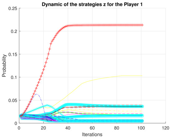
Figure 1. Convergence of strategies $z_{imk{k}^{\prime }}$ for player 1.

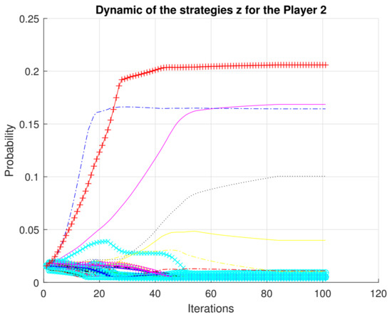
Figure 2. Convergence of strategies $z_{imk{k}^{\prime }}$ for player 2.

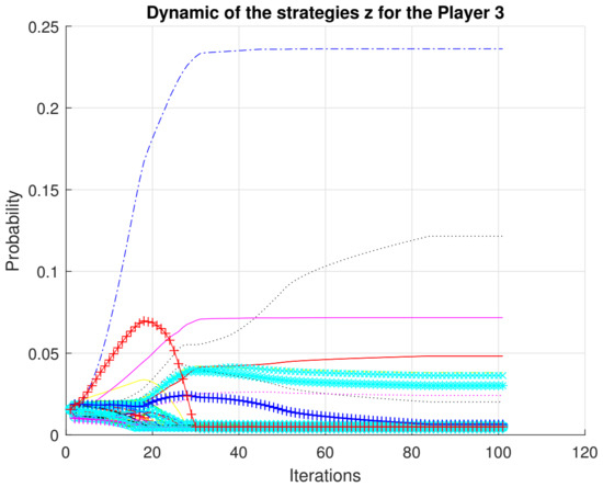
Figure 3. Convergence of strategies $z_{imk{k}^{\prime }}$ for player 3.

7. Conclusions

This paper contributed to the literature on mechanism design for Markov games with incomplete state information (partially observable). We suggested an analytical method for the design of a mechanism. The main result of this work is based on the introduction of the new variable z, which makes the game problem computationally tractable and allow for obtaining the mechanism solution $\mu$ and the strategies $\pi$ for all of the players in the game. The variable z allows for the introduction of new natural additional linear restrictions for computing the Nash equilibrium of the game. A no feasible solution can be detected with a simple test on the variable z, i.e., it is possible to detect unusual conditions in the solver of the game given the information available for the simplex. A major advantage of introducing this variable relies on the fact it can be efficiently implemented for real settings, which is consistent with the engineering approach for designing economic mechanisms or incentives, toward desired objectives, where players act rationally. We applied these results to a numerical example that is related to political promotion.

In relation to future work, there are several challenges that are left to address. One interesting technical challenge is that of addressing extremum seeking in the context of mechanism design [31,32,33]. Another interesting challenge would be to consider the observer design approach in order to extend the mechanism design theory [23].

References

- Hurwicz, L. Optimality and informational efficiency in resource allocation processes. In Mathematical Methods in the Social Sciences: Proceedings of the First Stanford Symposium; Arrow, K.J., Karlin, S., Suppes, P., Eds.; Stanford University Press: Palo Alto, CA, USA, 1960; pp. 27–46. [Google Scholar]
- Nobel. The Sveriges Riksbank Prize in Economic Sciences in Memory of Alfred Nobel 2007: Scientific Background; Technical Report; The Nobel Foundation: Stockholm, Sweden, 2007. [Google Scholar]
- Myerson, R.B. Allocation, Information and Markets; Chapter Mechanism Design; The New Palgrave; Palgrave Macmillan: London, UK, 1989; pp. 191–206. [Google Scholar]
- Vickrey, W. Counterspeculation, auctions, and competitive sealed tenders. J. Financ. 1961, 16, 8–37. [Google Scholar] [CrossRef]
- Bergemann, D.; Välimäki, J. Dynamic mechanism design: An introduction. J. Econ. Perspect 2019, 52, 235–274. [Google Scholar] [CrossRef]
- Clarke, E. Multi-part pricing of public goods. Public Choice 1971, 11, 17–23. [Google Scholar] [CrossRef]
- Groves, T. Incentives in teams. Econometrica 1973, 41, 617–631. [Google Scholar] [CrossRef]
- Harsanyi, J.C. Games with incomplete information played by bayesian players. part i: The basic model. Manag. Sci. 1967, 14, 159–182. [Google Scholar] [CrossRef]
- Arrow, K. Economics and Human Welfare; Chapter The Property Rights Doctrine and Demand Revelation under Incomplete Information; Academic Press: New York, NY, USA, 1979; pp. 23–39. [Google Scholar]
- D’Aspremont, C.; Gerard-Varet, L. Incentives and incomplete information. J. Public Econ. 1979, 11, 25–45. [Google Scholar]
- Saari, D.G. On the types of information and mechanism design. J. Comput. Appl. Math. 1988, 22, 231–242. [Google Scholar] [CrossRef][Green Version]
- Rogerson, W. Contractual solutions to the hold-up problem. Rev. Econ. Stud. 1992, 59, 777–793. [Google Scholar] [CrossRef]
- Mailath, G.; Postlewaite, A. Asymmetric information bargaining problems with many agents. Rev. Econ. Stud. 1990, 57, 351–360. [Google Scholar] [CrossRef]
- Miyakawa, T. Non-Cooperative Foundation of Nash Bargaining Solution under Incomplete Informational; Osaka University of Economics Working Paper Serier No. 2012-2.; Osaka University: Suita, Japan, 2012. [Google Scholar]
- Athey, S.; Bagwell, K. Collusion with persistent cost shocks. Econometrica 2008, 76, 493–540. [Google Scholar] [CrossRef]
- Hörner, J.; Takahashi, S.; Vieille, N. Truthful equilibria in dynamic bayesian games. Econometrica 2015, 83, 1795–1848. [Google Scholar] [CrossRef][Green Version]
- Clempner, J.B.; Poznyak, A.S. A nucleus for bayesian partially observable markov games: Joint observer and mechanism design. Eng. Appl. Artif. Intell. 2020, 95, 103876. [Google Scholar] [CrossRef]
- Rahman, D. The power of communication. Am. Econ. Rev. 2014, 104, 3737–3751. [Google Scholar] [CrossRef]
- Bernheim, B.; Madsen, E. Price cutting and business stealing in imperfect cartels. Am. Econ. Rev. 2017, 107, 387–424. [Google Scholar] [CrossRef][Green Version]
- Escobar, J.F.; Llanes, G. Cooperation dynamics in repeated games of adverse selection. J. Econ. Theory 2018, 176, 408–443. [Google Scholar] [CrossRef]
- Poznyak, A.S.; Najim, K.; Gómez-Ramírez, E. Self-Learning Control of Finite Markov Chains; Marcel Dekker, Inc.: New York, NY, USA, 2000. [Google Scholar]
- Clempner, J.B.; Poznyak, A.S. Simple computing of the customer lifetime value: A fixed local-optimal policy approach. J. Syst. Sci. Syst. Eng. 2014, 23, 439–459. [Google Scholar] [CrossRef]
- Clempner, J.B.; Poznyak, A.S. Observer and control design in partially observable finite markov chains. Automatica 2019, 110, 108587. [Google Scholar] [CrossRef]
- Clempner, J.B. On lyapunov game theory equilibrium: Static and dynamic approaches. Int. Game Theory Rev. 2018, 20, 1750033. [Google Scholar] [CrossRef]
- Clempner, J.B.; Poznyak, A.S. Finding the strong nash equilibrium: Computation, existence and characterization for markov games. J. Optim. Theory Appl. 2020, 186, 1029–1052. [Google Scholar] [CrossRef]
- Sragovich, V.G. Mathematical Theory of Adaptive Control; World Scientific Publishing Company: Singapore, 2006. [Google Scholar]
- Asiain, E.; Clempner, J.B.; Poznyak, A.S. A reinforcement learning approach for solving the mean variance customer portfolio for partially observable models. Int. J. Artif. Intell. Tools 2018, 27, 1850034-1–1850034-30. [Google Scholar] [CrossRef]
- Trejo, K.K.; Clempner, J.B.; Poznyak, A.S. Computing the lp-strong nash equilibrium for markov chains games. Appl. Math. Model. 2017, 41, 399–418. [Google Scholar] [CrossRef]
- Hotelling, H. Stability in competition. Econ. J. 1929, 39, 41–57. [Google Scholar] [CrossRef]
- Downs, A. An Economic Theory of Democracy; Harper & Brothers: New York, NY, USA, 1957. [Google Scholar]
- Solis, C.; Clempner, J.B.; Poznyak, A.S. Robust extremum seeking for a second order uncertain plant using a sliding mode controller. Int. J. Appl. Math. Comput. Sci. 2019, 29, 703–712. [Google Scholar] [CrossRef]
- Solis, C.; Clempner, J.B.; Poznyak, A.S. Robust integral sliding mode controller for optimisation of measurable cost functions with constraints. Int. J. Control 2019, 1–13, To be published. [Google Scholar] [CrossRef]
- Solis, C.; Clempner, J.B.; Poznyak, A.S. Continuous-time gradient-like descent algorithm for constrained convex unknown functions: Penalty method application. J. Comput. Appl. Math. 2019, 355, 268–282. [Google Scholar] [CrossRef]
Publisher’s Note: MDPI stays neutral with regard to jurisdictional claims in published maps and institutional affiliations. |
© 2021 by the authors. Licensee MDPI, Basel, Switzerland. This article is an open access article distributed under the terms and conditions of the Creative Commons Attribution (CC BY) license (http://creativecommons.org/licenses/by/4.0/).