
A Hierarchical Fuzzy-Based Correction Algorithm for the Neighboring Network Hit Problem †


Abstract
1. Introduction
1.1. Definitions
1.2. Context, Purpose, and Significance
- A novel and improved fuzzy logic methods for fixing erroneous CDRs and computing trips and distance.
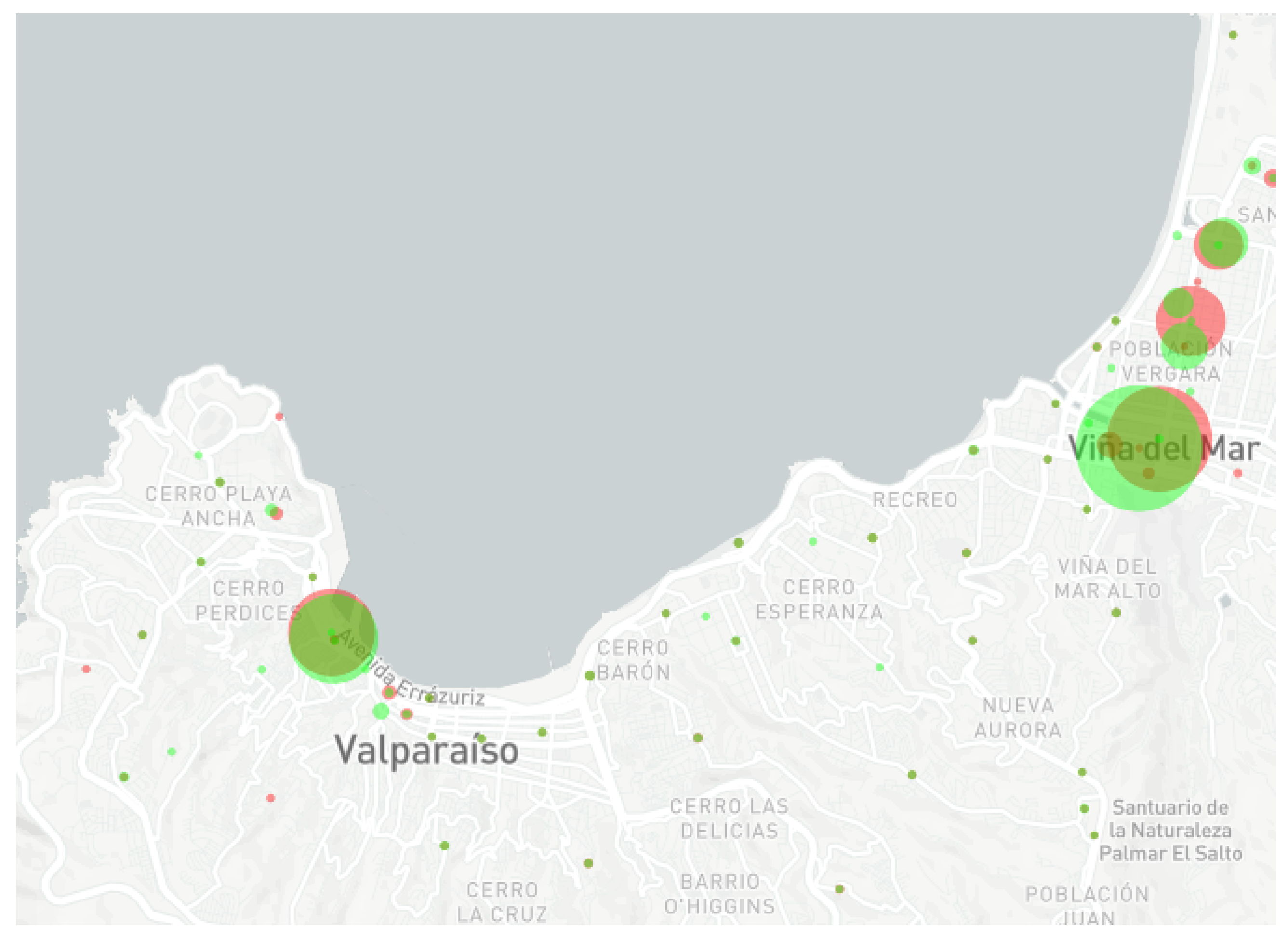
- A detailed evaluation of our methods using real-world based on data from Valparaíso Chile.
- A detailed evaluation of our methods with a real use case.
2. Understanding the Network and Its Limitations as a Mobility Data Source
2.1. The Problem
3. Related Work
3.1. Research Effort Using Cellular Data
3.2. Open Challenges and Opportunities Related to the Use of CDRs
3.3. Data Quality
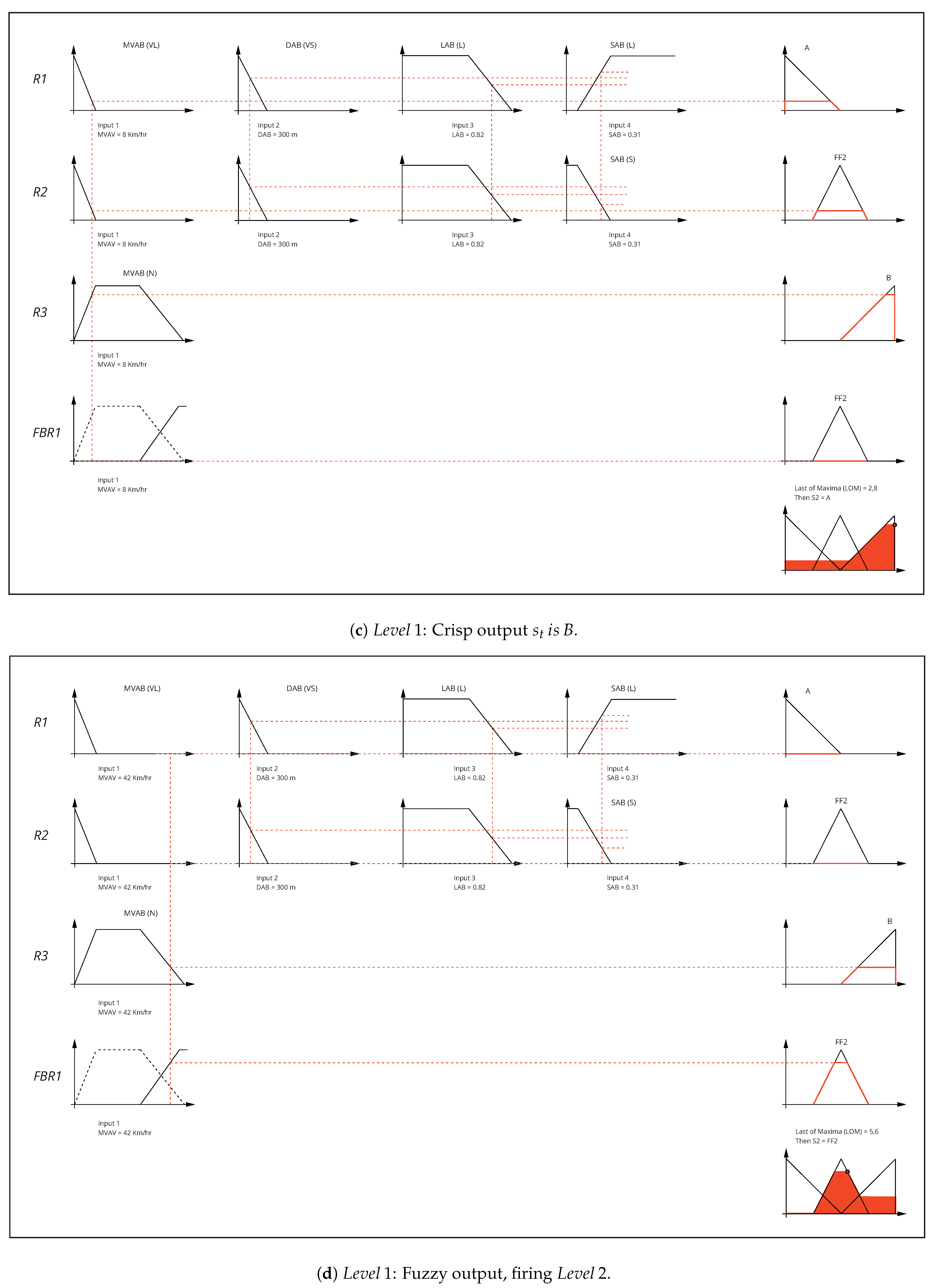
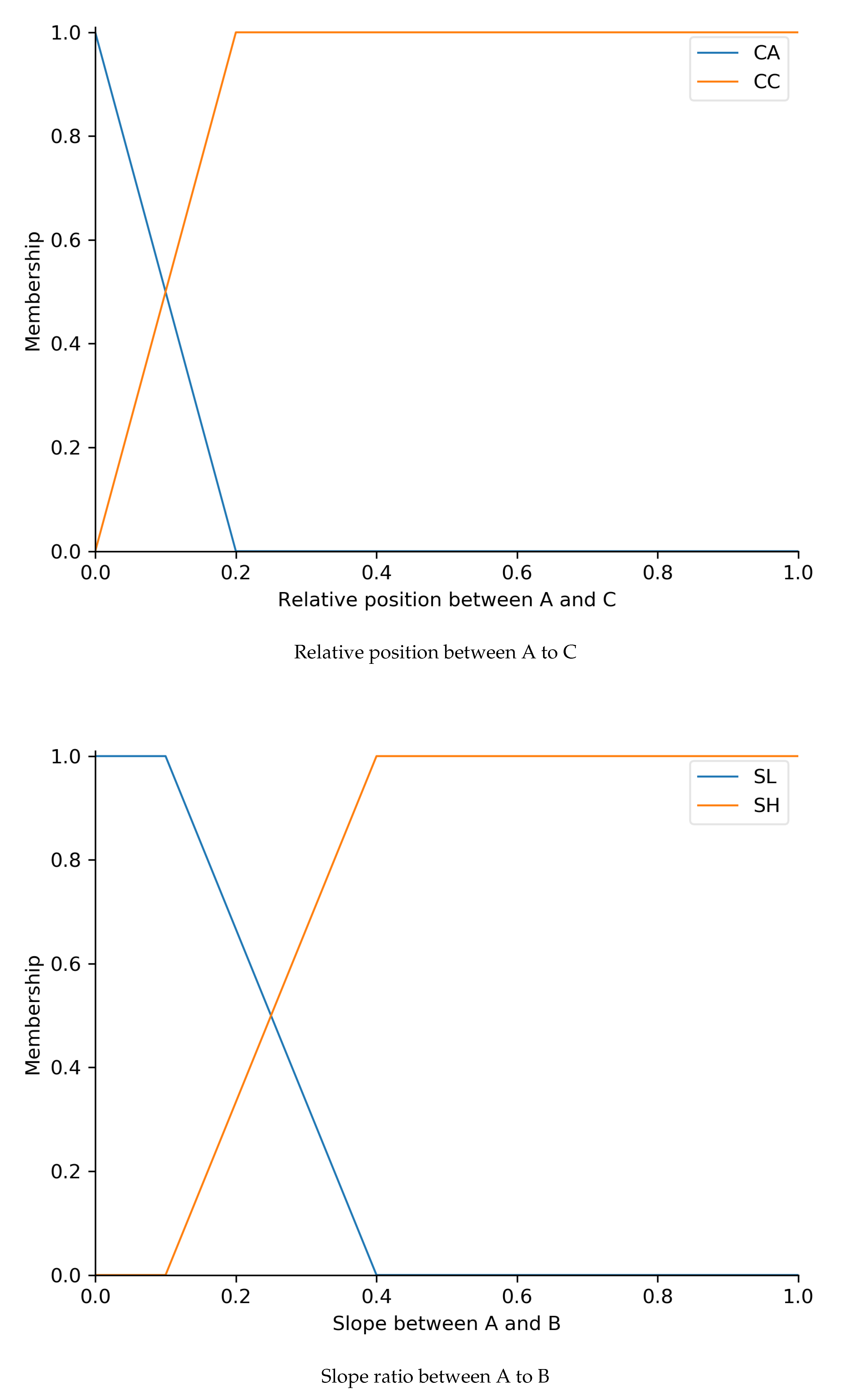
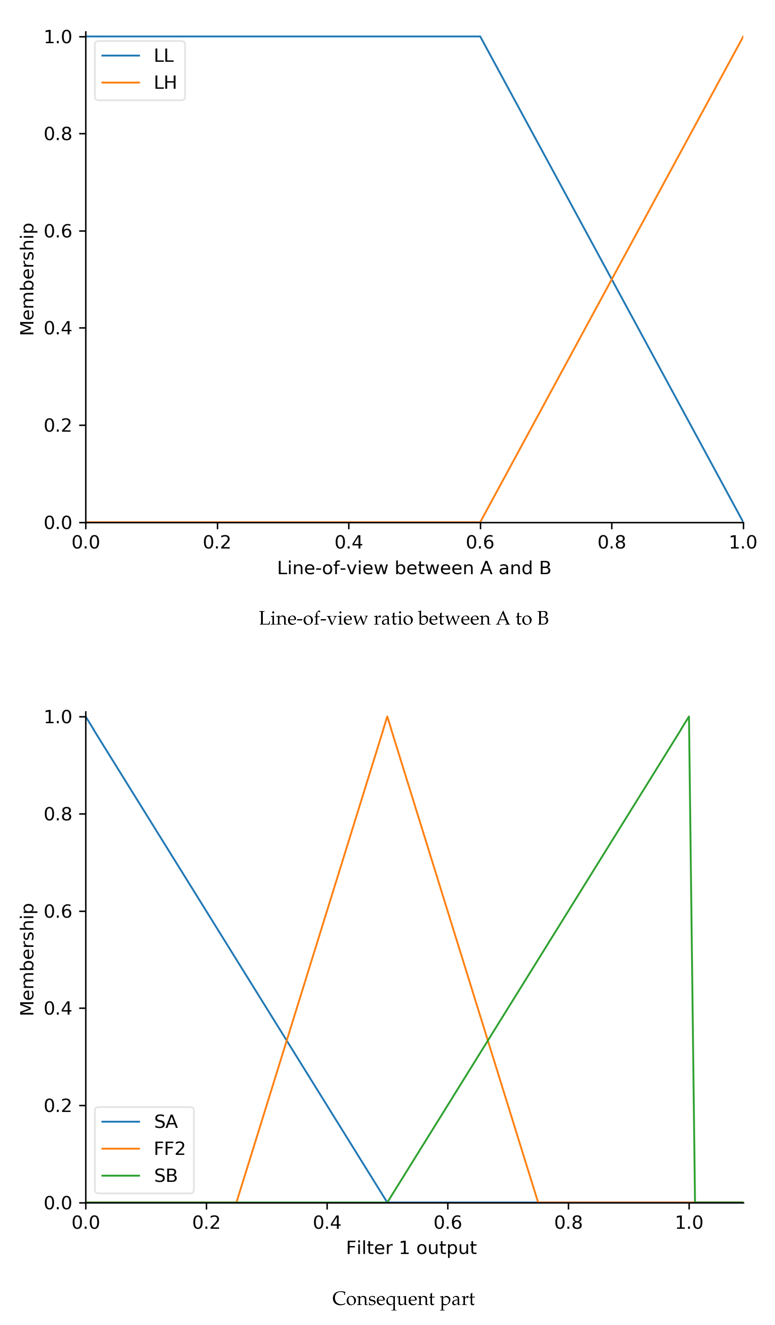
4. Fuzzy Reasoning Solution Approach
4.1. Fuzzy NNH Fix Algorithm (FNFA)
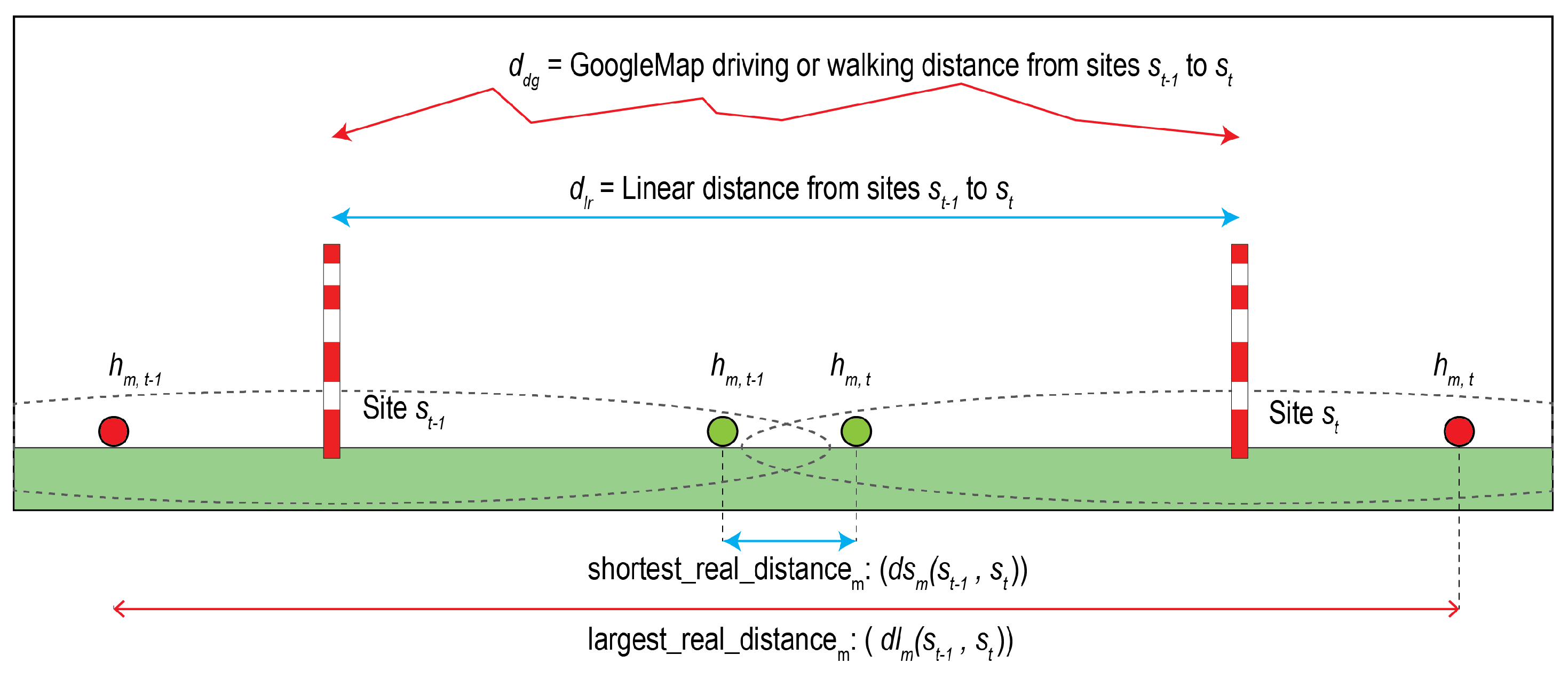
4.2. Fuzzy Trips Counting Algorithm (FTCA)
5. Experiment Setup
5.1. Input Data Description
5.2. Approach
6. Evaluation Results
6.1. Origin-Destination Survey (ODS)
6.2. Synthetic Data
6.3. Applying FNFA and FTCA to Small Groups of Data
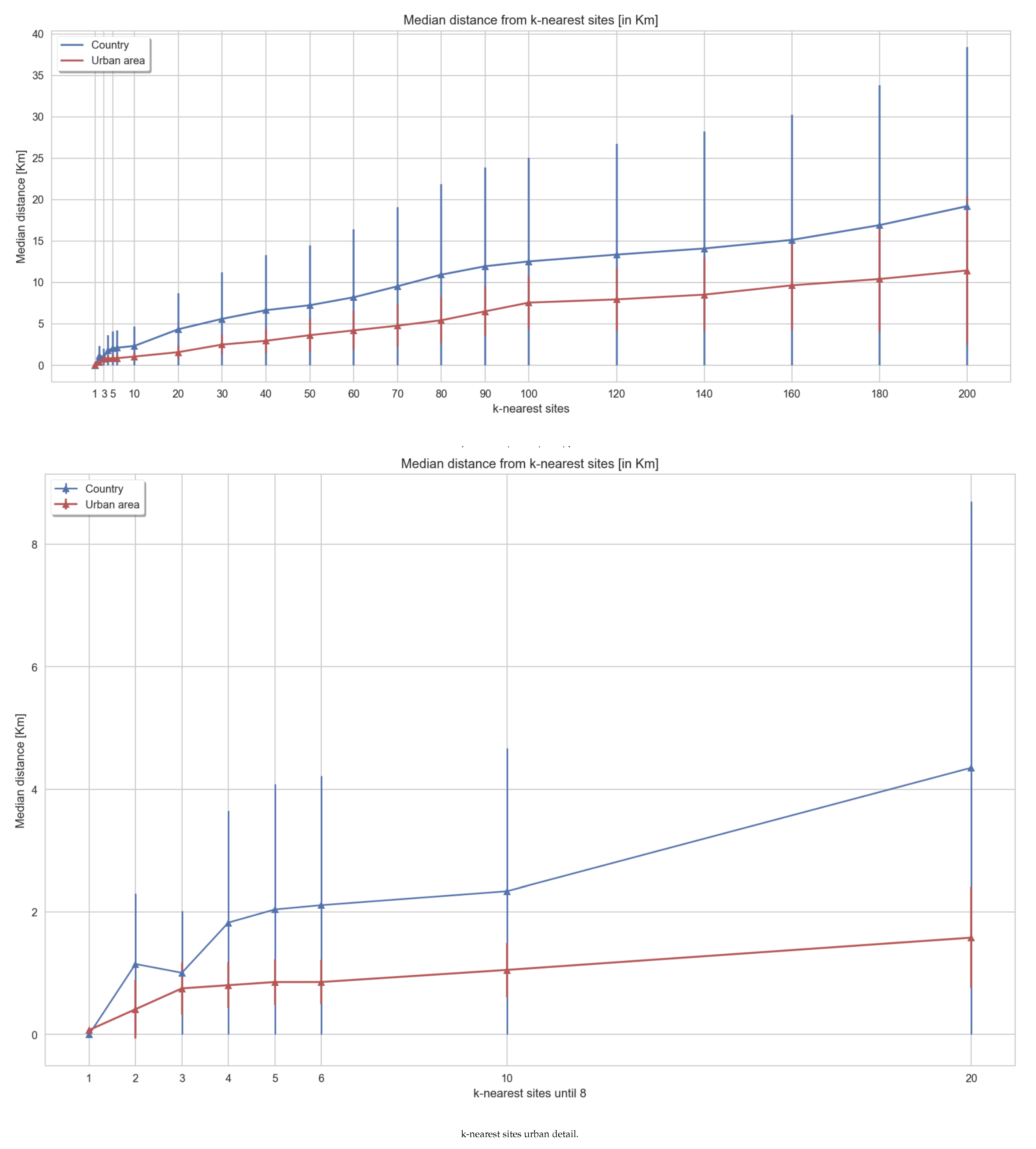
6.3.1. Computing Better Distance Distributions in Small Groups
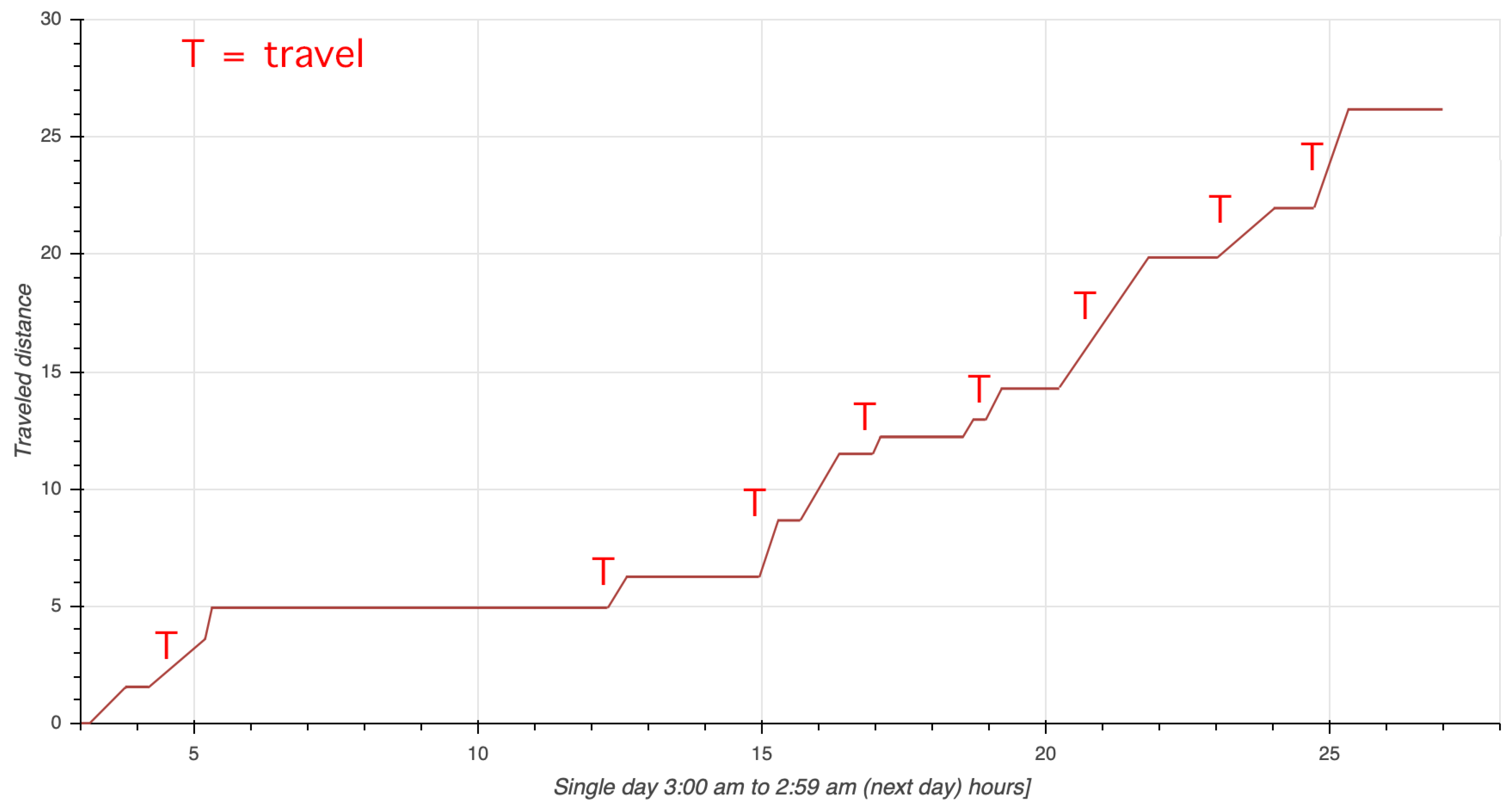
6.3.2. Analyzing Travels and Distance Distributions in Small Groups
7. Future Work and Conclusions
Author Contributions
Funding
Institutional Review Board Statement
Informed Consent Statement
Data Availability Statement
Conflicts of Interest
References
- Pinelli, F.; Di Lorenzo, G.; Calabrese, F. Comparing urban sensing applications using event and network-driven mobile phone location data. In Proceedings of the 2015 16th IEEE International Conference on Mobile Data Management, Pittsburgh, PA, USA, 15–18 June 2015; Volume 1, pp. 219–226. [Google Scholar]
- Graells-Garrido, E.; Peredo, O.; García, J. Sensing urban patterns with antenna mappings: The case of Santiago, Chile. Sensors 2016, 16, 1098. [Google Scholar] [CrossRef] [PubMed]
- Calabrese, F.; Ferrari, L.; Blondel, V.D. Urban sensing using mobile phone network data: A survey of research. ACM Comput. Surv. 2015, 47, 25. [Google Scholar] [CrossRef]
- Gakenheimer, R. Urban mobility in the developing world. Transp. Res. Part Policy Pract. 1999, 33, 671–689. [Google Scholar] [CrossRef]
- Oliver, N.; Lepri, B.; Sterly, H.; Lambiotte, R.; Deletaille, S.; De Nadai, M.; Letouzé, E.; Salah, A.A.; Benjamins, R.; Cattuto, C.; et al. Mobile phone data for informing public health actions across the COVID-19 pandemic life cycle. Sci. Adv. 2020, 6. [Google Scholar] [CrossRef]
- Groves, R.M. Nonresponse rates and nonresponse bias in household surveys. Public Opin. Q. 2006, 70, 646–675. [Google Scholar] [CrossRef]
- Kuwahara, M.; Sullivan, E.C. Estimating origin-destination matrices from roadside survey data. Transp. Res. Part Methodol. 1987, 21, 233–248. [Google Scholar] [CrossRef]
- Intelligence, G. Definitive Data and Analysis for the Mobile Industry. GSMA-Intelligence. 2019. Available online: https://www.gsma.com/services/wp-content/uploads/2019/06/GSMAIntelligence_Product_Brochure_2019.pdf (accessed on 5 December 2020).
- Blondel, V.D.; Decuyper, A.; Krings, G. A survey of results on mobile phone datasets analysis. EPJ Data Sci. 2015, 4, 10. [Google Scholar] [CrossRef]
- Pan, G.; Qi, G.; Zhang, W.; Li, S.; Wu, Z.; Yang, L.T. Trace analysis and mining for smart cities: Issues, methods, and applications. IEEE Commun. Mag. 2013, 51, 120–126. [Google Scholar] [CrossRef]
- Gonzalez, M.C.; Hidalgo, C.A.; Barabasi, A.L. Understanding individual human mobility patterns. Nature 2008, 453, 779. [Google Scholar] [CrossRef]
- Calabrese, F.; Pereira, F.C.; Di Lorenzo, G.; Liang, L.; Ratti, C. The geography of taste: Analyzing cell-phone mobility and social events. In International Conference on Pervasive Computing; Springer: Berlin/Heidelberg, Germany, 2010; Volume 10, pp. 22–37. [Google Scholar]
- Song, C.; Qu, Z.; Blumm, N.; Barabási, A.L. Limits of predictability in human mobility. Science 2010, 327, 1018–1021. [Google Scholar] [CrossRef]
- Leiva-Araos, A.; Allende-Cid, H.; Khryashchev, D.; Vo, H.T. Tackling the Neighboring Network Hit Problem in Cellular Data. In Proceedings of the 2019 IEEE International Conference on Big Data (Big Data), Los Angeles, CA, USA, 9–12 December 2019; pp. 2344–2353. [Google Scholar]
- Zimmermann, H. OSI reference model—The ISO model of architecture for open systems interconnection. IEEE Trans. Commun. 1980, 28, 425–432. [Google Scholar] [CrossRef]
- Damnjanovic, A.; Montojo, J.; Wei, Y.; Ji, T.; Luo, T.; Vajapeyam, M.; Yoo, T.; Song, O.; Malladi, D. A survey on 3GPP heterogeneous networks. IEEE Wirel. Commun. 2011, 18, 10–21. [Google Scholar] [CrossRef]
- De Jonge, E.; van Pelt, M.; Roos, M. Time Patterns, Geospatial Clustering and Mobility Statistics Based on Mobile Phone Network Data; Statistics Netherlands: The Hague, The Netherlands, 2012.
- Song, C.; Koren, T.; Wang, P.; Barabási, A.L. Modelling the scaling properties of human mobility. Nat. Phys. 2010, 6, 818. [Google Scholar] [CrossRef]
- Wang, D.; Pedreschi, D.; Song, C.; Giannotti, F.; Barabasi, A.L. Human mobility, social ties, and link prediction. In Proceedings of the 17th ACM SIGKDD, International Conference on Knowledge Discovery and Data Mining, San Diego, CA, USA, 21–24 August 2011; pp. 1100–1108. [Google Scholar]
- Isaacman, S.; Becker, R.; Cáceres, R.; Martonosi, M.; Rowland, J.; Varshavsky, A.; Willinger, W. Human mobility modeling at metropolitan scales. In Proceedings of the 10th International Conference on Mobile Systems, Applications, and Services, Low Wood Bay, Ambleside, UK, 25–29 June 2012; pp. 239–252. [Google Scholar]
- Mir, D.J.; Isaacman, S.; Cáceres, R.; Martonosi, M.; Wright, R.N. Dp-where: Differentially private modeling of human mobility. In Proceedings of the 2013 IEEE International Conference on Big Data, Silicon Valley, CA, USA, 6–9 October 2013; pp. 580–588. [Google Scholar]
- Graells-Garrido, E.; García, J. Visual exploration of urban dynamics using mobile data. In International Conference on Ubiquitous Computing and Ambient Intelligence; Springer: Cham, Switzerland, 2015; pp. 480–491. [Google Scholar]
- Graells-Garrido, E.; Ferres, L.; Caro, D.; Bravo, L. The effect of Pokémon Go on the pulse of the city: A natural experiment. EPJ Data Sci. 2017, 6, 23. [Google Scholar] [CrossRef]
- Isaacman, S.; Becker, R.; Cáceres, R.; Kobourov, S.; Martonosi, M.; Rowland, J.; Varshavsky, A. Identifying important places in people’s lives from cellular network data. In International Conference on Pervasive Computing; Springer: Berlin/Heidelberg, Germany, 2011; pp. 133–151. [Google Scholar]
- Reades, J.; Calabrese, F.; Sevtsuk, A.; Ratti, C. Cellular census: Explorations in urban data collection. IEEE Pervasive Comput. 2007, 6, 30–38. [Google Scholar] [CrossRef]
- Onnela, J.P.; Saramäki, J.; Hyvönen, J.; Szabó, G.; Lazer, D.; Kaski, K.; Kertész, J.; Barabási, A.L. Structure and tie strengths in mobile communication networks. Proc. Natl. Acad. Sci. USA 2007, 104, 7332–7336. [Google Scholar] [CrossRef] [PubMed]
- Ferres, L. Problems and Opportunities of Working with a Telco’s Large Data Sets of Mobile Data. In Proceedings of the Companion Proceedings of The 2019 World Wide Web Conference, San Francisco, CA, USA, 13–17 May 2019; p. 229. [Google Scholar]
- Beiró, M.G.; Bravo, L.; Caro, D.; Cattuto, C.; Ferres, L.; Graells-Garrido, E. Shopping mall attraction and social mixing at a city scale. EPJ Data Sci. 2018, 7, 28. [Google Scholar] [CrossRef]
- Ferreira, N.; Poco, J.; Vo, H.T.; Freire, J.; Silva, C.T. Visual exploration of big spatio-temporal urban data: A study of new york city taxi trips. IEEE Trans. Vis. Comput. Graph. 2013, 19, 2149–2158. [Google Scholar] [CrossRef]
- Freire, J.; Bessa, A.; Chirigati, F.; Vo, H.; Zhao, K. Exploring What not to Clean in Urban Data: A Study Using New York City Taxi Trips. Data Eng. 2016, 39, 63–77. [Google Scholar]
- Intelligence, G. The Mobile Economy 2020 GSMA-Intelligence. 2021. Available online: https://data.gsmaintelligence.com/api-web/v2/research-file-download?id=51249388&file=2915-260220-Mobile-Economy.pdf (accessed on 5 December 2020).
- Lambiotte, R.; Blondel, V.D.; De Kerchove, C.; Huens, E.; Prieur, C.; Smoreda, Z.; Van Dooren, P. Geographical dispersal of mobile communication networks. Phys. A Stat. Mech. Its Appl. 2008, 387, 5317–5325. [Google Scholar] [CrossRef]
- Laetitia, G.; Michele, T.; Simone, P.; Young, A.; Adler, N.; Stefaan, V.; Ferres, L.; Ciro, C. Gender gaps in urban mobility. Palgrave Commun. 2020, 7, 1–3. [Google Scholar]
- Ahas, R.; Silm, S.; Järv, O.; Saluveer, E.; Tiru, M. Using mobile positioning data to model locations meaningful to users of mobile phones. J. Urban Technol. 2010, 17, 3–27. [Google Scholar] [CrossRef]
- Nurmi, P.; Bhattacharya, S. Identifying meaningful places: The non-parametric way. In International Conference on Pervasive Computing; Springer: Berlin/Heidelberg, Germany, 2008; pp. 111–127. [Google Scholar]
- Becker, R.A.; Caceres, R.; Hanson, K.; Loh, J.M.; Urbanek, S.; Varshavsky, A.; Volinsky, C. Route classification using cellular handoff patterns. In Proceedings of the 13th International Conference on Ubiquitous Computing, Beijing, China, 17–21 September 2011; pp. 123–132. [Google Scholar]
- Girardin, F.; Vaccari, A.; Gerber, A.; Biderman, A.; Ratti, C. Quantifying urban attractiveness from the distribution and density of digital footprints. Int. J. 2009, 4, 175–200. [Google Scholar]
- Soto, V.; Frias-Martinez, E. Robust land use characterization of urban landscapes using cell phone data. In Proceedings of the 1st Workshop on Pervasive Urban Applications, in Conjunction with 9th Int. Conf. Pervasive Computing, San Francisco, CA, USA, 12 June 12 2011. [Google Scholar]
- Farrahi, K.; Gatica-Perez, D. What did you do today? Discovering daily routines from large-scale mobile data. In Proceedings of the 16th ACM International Conference on Multimedia, Vancouver, BC, Canada, 26–31 October 2008; pp. 849–852. [Google Scholar]
- Buckee, C.O.; Balsari, S.; Chan, J.; Crosas, M.; Dominici, F.; Gasser, U.; Grad, Y.H.; Grenfell, B.; Halloran, M.E.; Kraemer, M.U.; et al. Aggregated mobility data could help fight COVID-19. Science 2020, 368, 145. [Google Scholar] [CrossRef]
- Steenbruggen, J.; Tranos, E.; Nijkamp, P. Data from mobile phone operators: A tool for smarter cities? Telecommun. Policy 2015, 39, 335–346. [Google Scholar] [CrossRef]
- Krisp, J.M. Planning fire and rescue services by visualizing mobile phone density. J. Urban Technol. 2010, 17, 61–69. [Google Scholar] [CrossRef]
- Peters, S.; Krisp, J.M. Density calculation for moving points. In Proceedings of the 13th AGILE International Conference on Geographic Information Science, Guimaraes, Portugal, 11–14 May 2010; Volume 1014. [Google Scholar]
- Soto, V.; Frias-Martinez, V.; Virseda, J.; Frias-Martinez, E. Prediction of socioeconomic levels using cell phone records. In International Conference on User Modeling, Adaptation, and Personalization; Springer: Berlin/Heidelberg, Germany, 2011; pp. 377–388. [Google Scholar]
- Simini, F.; González, M.C.; Maritan, A.; Barabási, A.L. A universal model for mobility and migration patterns. Nature 2012, 484, 96–100. [Google Scholar] [CrossRef] [PubMed]
- Wang, P.; Hunter, T.; Bayen, A.M.; Schechtner, K.; González, M.C. Understanding road usage patterns in urban areas. Sci. Rep. 2012, 2, 1001. [Google Scholar] [CrossRef]
- Calabrese, F.; Colonna, M.; Lovisolo, P.; Parata, D.; Ratti, C. Real-time urban monitoring using cell phones: A case study in Rome. IEEE Trans. Intell. Transp. Syst. 2011, 12, 141–151. [Google Scholar] [CrossRef]
- Lu, X.; Wetter, E.; Bharti, N.; Tatem, A.J.; Bengtsson, L. Approaching the limit of predictability in human mobility. Sci. Rep. 2013, 3, 1–9. [Google Scholar] [CrossRef] [PubMed]
- Bagrow, J.P.; Wang, D.; Barabasi, A.L. Collective response of human populations to large-scale emergencies. PLoS ONE 2011, 6, e17680. [Google Scholar] [CrossRef] [PubMed]
- Lu, X.; Bengtsson, L.; Holme, P. Predictability of population displacement after the 2010 Haiti earthquake. Proc. Natl. Acad. Sci. USA 2012, 109, 11576–11581. [Google Scholar] [CrossRef] [PubMed]
- Ferrari, L.; Mamei, M.; Colonna, M. People get together on special events: Discovering happenings in the city via cell network analysis. In Proceedings of the 2012 IEEE International Conference on Pervasive Computing and Communications Workshops, Lugano, Switzerland, 19–23 March 2012; pp. 223–228. [Google Scholar]
- Traag, V.A.; Browet, A.; Calabrese, F.; Morlot, F. Social event detection in massive mobile phone data using probabilistic location inference. In Proceedings of the 2011 IEEE Third International Conference on Privacy, Security, Risk and Trust and 2011 IEEE Third International Conference on Social Computing, Boston, MA, USA, 9–11 October 2011; pp. 625–628. [Google Scholar]
- Blondel, V.; Krings, G.; Thomas, I. Regions and borders of mobile telephony in Belgium and in the Brussels metropolitan zone. Brussels Studies. La Revue Scientifique électronique pour les Recherches sur Bruxelles/Het Elektronisch Wetenschappelijk Tijdschrift voor Onderzoek over Brussel/ J. Acad. Res. Bruss. 2010. [Google Scholar] [CrossRef]
- Calabrese, F.; Dahlem, D.; Gerber, A.; Paul, D.; Chen, X.; Rowland, J.; Rath, C.; Ratti, C. The connected states of america: Quantifying social radii of influence. In Proceedings of the 2011 IEEE Third International Conference on Privacy, Security, Risk and Trust and 2011 IEEE Third International Conference on Social Computing, Boston, MA, USA, 9–11 October 2011; pp. 223–230. [Google Scholar]
- Couronne, T.; Olteanu, A.M.; Smoreda, Z. Urban mobility: Velocity and uncertainty in mobile phone data. In Proceedings of the 2011 IEEE Third International Conference on Privacy, Security, Risk and Trust and 2011 IEEE Third International Conference on Social Computing, Boston, MA, USA, 9–11 October 2011; pp. 1425–1430. [Google Scholar]
- Pokhriyal, N.; Dong, W.; Govindaraju, V. Virtual networks and poverty analysis in senegal. arXiv 2015, arXiv:1506.03401. [Google Scholar]
- Martinez-Cesena, E.A.; Mancarella, P.; Ndiaye, M.; Schläpfer, M. Using mobile phone data for electricity infrastructure planning. arXiv 2015, arXiv:1504.03899. [Google Scholar]
- Hossain, S.; Abtahee, A.; Kashem, I.; Hoque, M.M.; Sarker, I.H. Crime Prediction Using Spatio-Temporal Data. In International Conference on Computing Science, Communication and Security; Springer: Berlin/Heidelberg, Germany, 2020; pp. 277–289. [Google Scholar]
- Klein, B.; LaRocky, T.; McCabey, S.; Torresy, L.; Privitera, F.; Lake, B.; Kraemer, M.U.; Brownstein, J.S.; Lazer, D.; Eliassi-Rad, T.; et al. Assessing Changes in Commuting and Individual Mobility in Major Metropolitan Areas in the United States during the COVID-19 Outbreak. Network Science Institute, Northeastern University. 31 March 2020. Available online: https://uploads-ssl.webflow.com/5c9104426f6f88ac129ef3d2/5e8374ee75221201609ab586_Assessing_mobility_changes_in_the_United_States_during_the_COVID_19_outbreak.pdf (accessed on 5 December 2020).
- Zhao, K.; Tarkoma, S.; Liu, S.; Vo, H. Urban human mobility data mining: An overview. In Proceedings of the 2016 IEEE International Conference on Big Data (Big Data), Washington, DC, USA, 5–8 December 2016; pp. 1911–1920. [Google Scholar]
- Zadeh, L.A. Information and control. Fuzzy Sets 1965, 8, 338–353. [Google Scholar]
- Mamdani, E.H. Application of fuzzy algorithms for control of simple dynamic plant. In Proceedings of the Institution of Electrical Engineers; IET: London, UK, 1974; Volume 121, pp. 1585–1588. [Google Scholar] [CrossRef]
- De Luca, A.; Termini, S. A definition of a nonprobabilistic entropy in the setting of fuzzy sets theory. In Readings in Fuzzy Sets for Intelligent Systems; Elsevier: Amsterdam, The Netherlands, 1993; pp. 197–202. [Google Scholar]
- Dubois, D.J. Fuzzy Sets and Systems: Theory and Applications; Academic Press: Cambridge, MA, USA, 1980; Volume 144. [Google Scholar]
- Torra, V. A review of the construction of hierarchical fuzzy systems. Int. J. Intell. Syst. 2002, 17, 531–543. [Google Scholar] [CrossRef]
- Stufflebeam, J.; Prasad, N.R. Hierarchical fuzzy control. In Proceedings of the FUZZ-IEEE’99. 1999 IEEE International Fuzzy Systems. Conference Proceedings (Cat. No. 99CH36315), Seoul, Korea, 22–25 August 1999; Volume 1, pp. 498–503. [Google Scholar]
- Yager, R.R. On a hierarchical structure for fuzzy modeling and control. IEEE Trans. Syst. Man, Cybern. 1993, 23, 1189–1197. [Google Scholar] [CrossRef]
- Jamshidi, M. Large-Scale Systems: Modeling, Control, and Fuzzy Logic; Prentice-Hall, Inc.: New Jersey, NJ, USA, 1996. [Google Scholar]
- Takagi, T.; Sugeno, M. Fuzzy identification of systems and its applications to modeling and control. IEEE Trans. Syst. Man Cybern. 1985, 116–132. [Google Scholar] [CrossRef]
- Li, X.; Pan, G.; Wu, Z.; Qi, G.; Li, S.; Zhang, D.; Zhang, W.; Wang, Z. Prediction of urban human mobility using large-scale taxi traces and its applications. Front. Comput. Sci. 2012, 6, 111–121. [Google Scholar]
- Hurtado, O.S.U.A. Informe Ejecutivo, EOD de Viajes—Santiago 2012; Biblioteca Sectra: Santiago, Chile, 2015. [Google Scholar]
- Kong, X.; Li, M.; Ma, K.; Tian, K.; Wang, M.; Ning, Z.; Xia, F. Big trajectory data: A survey of applications and services. IEEE Access 2018, 6, 58295–58306. [Google Scholar] [CrossRef]
- Zarsky, T.Z. Incompatible: The GDPR in the age of big data. Seton Hall L. Rev. 2016, 47, 995. [Google Scholar]


| Study Reference | Case Study | NNH Treatment | Data |
|---|---|---|---|
| [2,22] | Human mobility exploration | Record deleting | Pre-processed |
| [3] | Survey of mobility | Mentioned as critical | NA |
| [11,18] | Human mobility patters | Not mentioned | Controlled sample |
| [12] | Mobility during social events | Spatial isolation | Pre-processed |
| [20,21] | Synthetic data generation | Not mentioned | Controlled sample |
| [23] | Impact of location-based game in the pulse of a city | Record deleting | Pre-processed |
| [24] | Semantic places in people’s lives | Not mentioned | Controlled sample |
| [25] | City as a holistic, dynamic system | Not mentioned | Pre-processed |
| [26] | Local and the global structure of a society-wide communication network | Not mentioned | Pre-processed |
| [27] | Data science for social good | Record deleting | Pre-processed |
| [28] | Mobility and social inclusion | Record deleting | Pre-processed |
| [29] | Taxi trips visual exploration | Mentioned, record deleting | Raw data |
| [30] | Taxi trips data cleaning | Domain Knowledge | Raw data |
| Variable Name | Universe of Discourse | Linguistic Terms |
|---|---|---|
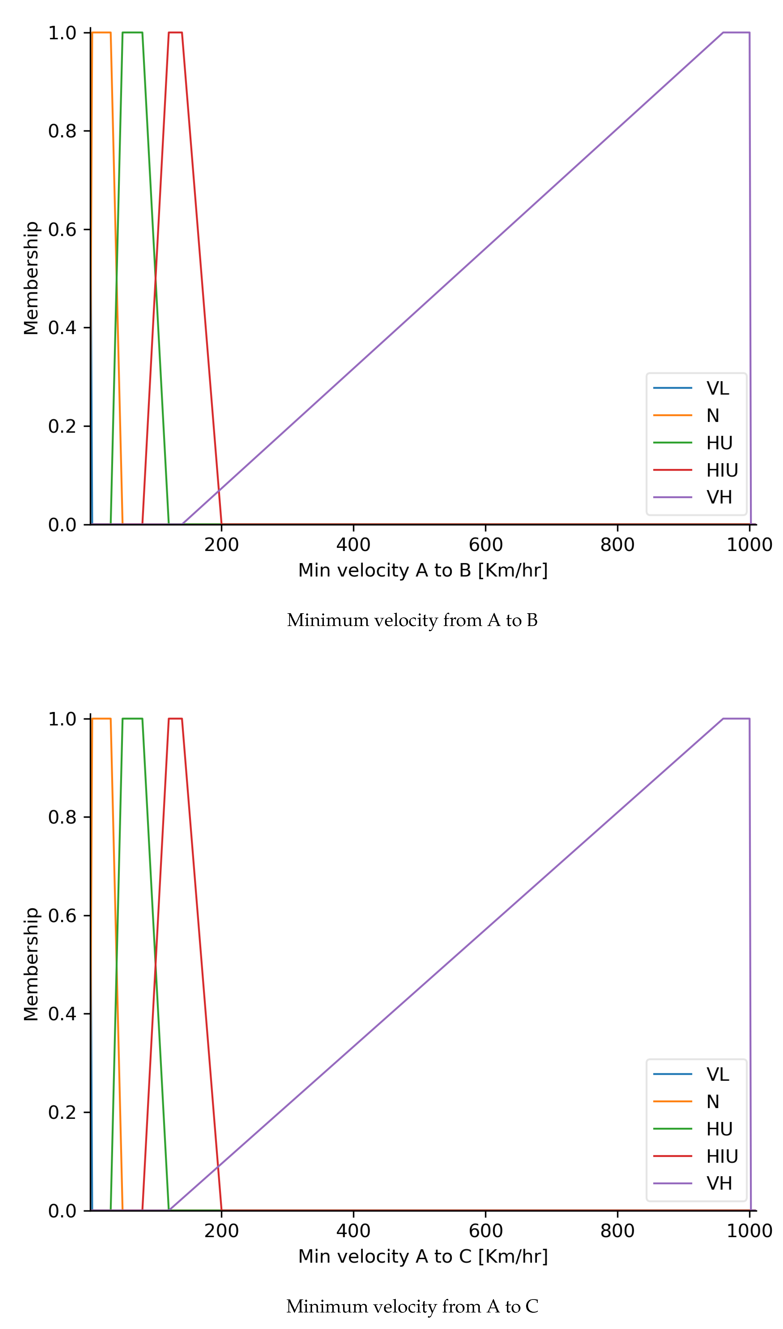
| , [km/h] | ||
| , [km/h] | ||
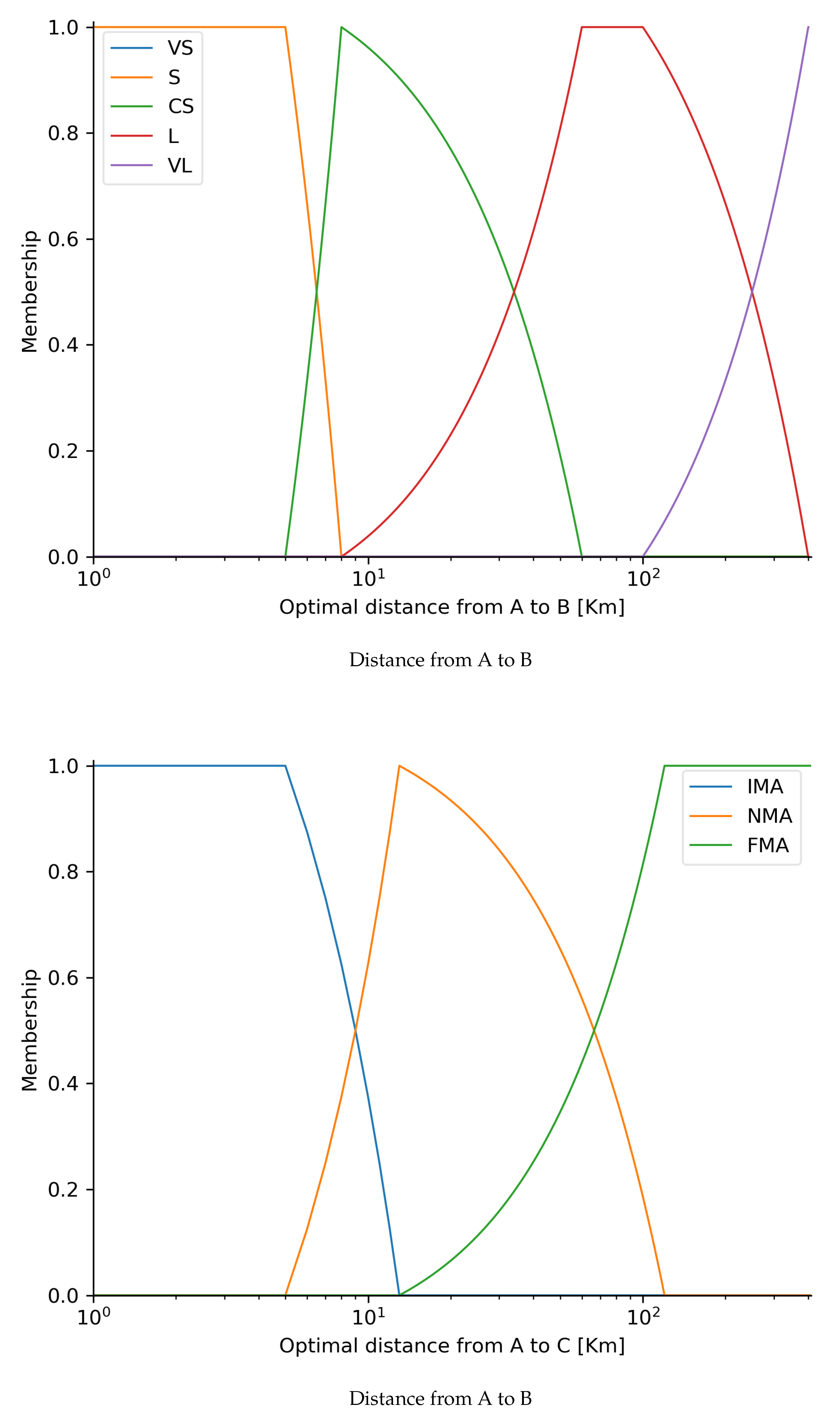
| , [km] | ||
| , [km] | ||
| , [km] | ||
| , [km] |
| Variable Name | Universe of Discourse | Linguistic Terms |
|---|---|---|
| , [h] | ||
| , [min] | ||
| Records Statistics after Filter Devices with NH = 1 | ||||||
|---|---|---|---|---|---|---|
| City: Date | Count () | NH/ device | NH/ device | Dev. NH > 1 () | Dev. NH = 1 () | |
| Val: 17/01/01 | 10.3 | 41.2 | 44 | 62.1 | 250 | 19 |
| Val: 18/01/01 | 11.9 | 37.8 | 35 | 83.7 | 314 | 146 |
| Val: 17/06/03 | 9.7 | 46.6 | 45 | 122.3 | 209 | 15 |
| Val: 18/01/03 | 8.8 | 29.6 | 22 | 65.6 | 299 | 143 |
| 40.7 | ||||||
| Inhabitants | Travels/Day | Sampled Homes | Year | Average Travels | |
|---|---|---|---|---|---|
| () | () | () | Study | /Day-Person | |
| Santiago | 6652 | 18,461 | 18,264 | 2012 | 2.78 |
| Valparaíso | 928 | 2248 | 6800 | 2014 | 2.27 |
| Concepción | N/A | N/A | 8400 | 2015 | N/A |
| Homes | People | Travels/Day | Average Travels | |
|---|---|---|---|---|
| /Day-Person | ||||
| Con-Con | 13.8 | 47.4 | 118.6 | 2.50 |
| Viña del Mar | 109.4 | 321.8 | 852.2 | 2.67 |
| Valparaíso | 98.4 | 259.1 | 697.3 | 2.36 |
| Quilpué | 49.1 | 165.3 | 348.4 | 2.11 |
| Villa Alemana | 36.5 | 135.0 | 231.6 | 1.72 |
| Total | 307.2 | 928.6 | 2248.1 | 2.27 |
| 1 January 2018 | 6 March 2017 | ||||||||
|---|---|---|---|---|---|---|---|---|---|
| Experiment | Set of algorithms | Fixed NNH | % fixed records | Traces | Trips | Fixed NNH | % fixed records | Traces | Trips |
| Raw data | TCA | 0 | 0.00 | 7.96 | 2.53 | 0 | 0.00 | 7.08 | 2.48 |
| NFA-TCA | 412,235 | 3.71 | 6.95 | 2.42 | 259,370 | 2.70 | 6.27 | 2.38 | |
| NFA-TCA | 432,301 | 3.89 | 6.90 | 2.42 | 271,720 | 2.83 | 6.23 | 2.37 | |
| FNFA-FTCA | 610,111 | 5.49 | 6.06 | 2.25 | 383,096 | 3.99 | 6.02 | 2.29 | |
| NFA-TCA | 457,942 | 4.12 | 6.83 | 2.39 | 288,164 | 3.00 | 6.18 | 2.36 | |
| NFA-TCA | 494,580 | 4.45 | 6.74 | 2.39 | 311,901 | 3.25 | 6.11 | 2.35 | |
| NFA-TCA | 528,122 | 4.75 | 6.77 | 2.35 | 322,591 | 3.36 | 6.14 | 2.36 | |
| FNFA-FTCA | 706,015 | 6.35 | 6.58 | 2.30 | 476,206 | 4.96 | 5.95 | 2.31 | |
| NFA-TCA | 547,757 | 4.92 | 6.72 | 2.40 | 334,780 | 3.49 | 6.10 | 2.35 | |
| NFA-TCA | 631,110 | 5.67 | 6.59 | 2.39 | 375,286 | 3.91 | 6.01 | 2.34 | |
| NFA-TCA | 655,735 | 5.89 | 6.53 | 2.38 | 391,382 | 4.08 | 5.96 | 2.33 | |
| FNFA-FTCA | 760,652 | 6.83 | 6.01 | 2.21 | 454,003 | 4.73 | 5.48 | 2.16 | |
| NFA-TCA | 691,407 | 6.22 | 6.44 | 2.37 | 414,402 | 4.32 | 5.89 | 2.32 | |
Publisher’s Note: MDPI stays neutral with regard to jurisdictional claims in published maps and institutional affiliations. |
© 2021 by the authors. Licensee MDPI, Basel, Switzerland. This article is an open access article distributed under the terms and conditions of the Creative Commons Attribution (CC BY) license (http://creativecommons.org/licenses/by/4.0/).
Share and Cite
Leiva-Araos, A.; Allende-Cid, H. A Hierarchical Fuzzy-Based Correction Algorithm for the Neighboring Network Hit Problem. Mathematics 2021, 9, 315. https://doi.org/10.3390/math9040315
Leiva-Araos A, Allende-Cid H. A Hierarchical Fuzzy-Based Correction Algorithm for the Neighboring Network Hit Problem. Mathematics. 2021; 9(4):315. https://doi.org/10.3390/math9040315
Chicago/Turabian StyleLeiva-Araos, Andrés, and Héctor Allende-Cid. 2021. "A Hierarchical Fuzzy-Based Correction Algorithm for the Neighboring Network Hit Problem" Mathematics 9, no. 4: 315. https://doi.org/10.3390/math9040315
APA StyleLeiva-Araos, A., & Allende-Cid, H. (2021). A Hierarchical Fuzzy-Based Correction Algorithm for the Neighboring Network Hit Problem. Mathematics, 9(4), 315. https://doi.org/10.3390/math9040315