Price Competition and Setup Cost

Abstract

Few studies analyze the endogenous emergence of price competition in a new product market. This paper analyzes two differentiated products, an existing product and a newly introduced substitutable product, and investigates conditions under which a price competition endogenously emerges in a new product market in the context of a choice between engaging in price competition and holding price leadership. We demonstrate that Bertrand price competition emerges when the setup cost for the new product is high enough. This result implies that government policies reducing setup costs such as subsidies could change the type of competition to price leadership in a new product market.

1. Introduction

In a market where new products replace existing commodities, we often observe that an innovative firm and subsequent firms engage in price competition. For example, in the growth stage of smartphones, which have replaced cell phones worldwide, Sherman [1] reports that Apple and Samsung have moved into price wars: Apple’s iPhone 4 was just $270 in Brazil, and Samsung cut the price of Galaxy S models in Asia by nearly half. Despite this, little has been understood about the rationale behind the emergence of price competition until a study by Yano and Komatsubara [2], which demonstrates that Bertrand price competition emerges as a consequence of the active strategic behavior of firms in a duopoly market for a homogeneous product. As for the rationale of the emergence of price competition in a new product market, however, little has been studied in the existing literature. The present paper intends to explain a mechanism behind the emergence of price competition for a new product in a duopoly market in which consumers prefer a new product to an existing old product.

To this end, this study constructs an endogenous timing model in which both an existing product and a new product are available to consumers. Incorporating a substitutable old product in the model enables us to understand how different timings of an action, that is, pricing, affect the expansion of a new product in society. Ota [3] investigates the dynamic equilibrium pricing of an “old” product when the value of a new product emerges, after which the demand for the old product is gradually replaced by that for the new product. With an endogenous timing model, Yano and Komatsubara [2] provide conditions for the emergence of Bertrand price competition. Different from the study by Yano and Komatsubara [2], which analyzes a homogeneous-good duopoly market, this paper focuses on the emergence of price competition in a new product market in the context of a choice between engaging in price competition and holding price leadership.

In our duopoly model, an incumbent firm produces both old and new products, whereas an entrant firm produces the new product only. While the new product is homogeneous among firms, the old and new products are differentiated by the following two aspects. First, consumers distinguish these products by their marginal willingness to pay (MWP). We assume that the MWP for the new product is always higher than that for the old product for any consumer. Second, the production costs are different between the two products. To produce a new product, firms must pay not only a marginal cost but also a setup cost. The research and development cost is an example of a setup cost, and needless to say, it plays an essential role in introducing a new product.

Using this model, we demonstrate that the setup cost of the new product determines the timing of its pricing. In particular, Bertrand price competition emerges when the setup cost is high. Here, we explain the mechanism of this result by assuming that the marginal cost of the new product and that of the old product are the same. In order to analyze price competition in the framework of Hamilton and Slutsky [4], we follow Dastidar [5] assuming that each firm sells as much as the existing demand at its set price. Because the firms use the same technology, Dastidar [5]’s assumption implies that two firms divide the demand for the new product by half once they enter the market. Then, when the setup cost is high, firms cannot obtain a positive profit from half of the market demand at a price set by them. However, a firm can obtain a higher positive profit if it captures all the market demand by undercutting the price. That is, when the setup cost is high enough, Bertrand price competition emerges.

As discussed at the outset, the purpose of this study is to investigate the conditions under which a price competition endogenously emerges in a new product market. In the case of quantity competition, Amir and Grilo [6] and van Damme and Hurkens [7] analyze Cournot competition in the framework of Hamiltonand Slutsky [4]; these studies provide conditions yielding the simultaneous and the sequential move, respectively.

In this study, firms compete in terms of price only in a new product market. Because the new product is homogeneous, our study forms part of the literature on price competition in a homogeneous product market, for example, Ono [8], Tasnádi [9], Dastidar and Furth [10], Yano and Komatsubara [11], Komatsubara [12], and Hirata and Matsumura [13]. Different from these studies, this paper studies a differentiated product to analyze the common scenario in which a new product replaces an existing product. In this sense, our study is also related to the literature on endogenous timing games with heterogeneous products, such as van Damme and Hurkens [14] and Amir and Stepanova [15]. However, the focus of these papers is on an endogenous formation of price leadership according to risk dominance, which is not the aim of our research.

We build a model that incorporates a homogeneous product model and a differentiated product model and characterize the conditions under which price competition and price leadership emerge in the market where a new product and existing products are supplied. From the aspect of the homogeneous product model, which is adopted by Cabon-Dhersin and Drouhin [16] and Routledge and Edwards [17], our model shows that Bertrand price competition in a new product market appears depending on the size of the setup cost. While Dastidar [5] and Yano and Komatsubara [2] demonstrate that differences in marginal cost of firms play an important role to explain the emergence of Bertrand competition, our paper provides a new factor, non-sunk setup cost, for the appearance.

Our model also can be captured as a differentiated product model because we assumes that one firm supplies only a new product and the other supplies both new and existing products and characterizes pricing of them. From the aspect of the differentiated product model, this paper is close to Madden and Pezzino [18]. While that paper analyzes pricing of two complemented goods supplied by a firm, we investigate pricing of new and existing product that are substitutable.

The literature on industrial dynamics is also close to our paper. This study focuses on a market where a new product replaces existing commodities and investigates what type of price competition emerges in such a market. It is closely related to the literature on pricing in the market where new products are frequently launched. Lim and Tang [19] and Liang, Çakanyıldırım, and Sethi [20] examine pricing by a firm adopting a product launching strategy in which a new product is sold together with existing products in the market, so called dual-roll strategy. Broadly speaking, this study is also associated with the literature on product innovations in the field of endogenous growth such as Silverberg and Verspagen [21] and Furukawa [22].

This paper is organized as follows. In Section 2, we describe the market structure, where two firms compete in the price for a new product, although one of the firms can also produce an old product. Section 3 presents the analyses of the equilibrium of the model, and explanation of the conditions under which Bertrand price competition endogenously emerges. Section 4 discusses our results and presents the concluding remarks.

2. Differentiated Products Model

2.1. Firms and Consumers

In this section, we construct a model in which there are two firms and two products that are differentiated with respect to consumers’ willingness to pay and production costs. While firm 1 supplies both products, firm 2 supplies the new product only.

Let $q_1^N$ and $q_2^N$ denote the quantities of the new product supplied by firms 1 and 2, respectively. The market supply of the new product, $q^N,$ is the sum of the two, that is,

$$q_1^N+q_2^N=q^N.$$

(1)

Let $q^O$ denote the market supply of the old product by firm 1. Thus, the total number of products supplied by firms 1 and 2 is $q^N+q^O.$

In order to supply $q^N$ units of new products, each firm incurs the following costs: for firm $i=1,2,$

$$C(q_i^N)=\left\{\begin{array}{cc}c{q}_i^N+F& \mathrm{if}{q}_i^N>0\\ 0& \mathrm{if}{q}_i^N=0,\end{array}\right.$$

(2)

where a marginal cost $c\ge 0$ and a setup cost $F\ge 0$ are constant. The setup cost is not a sunk cost. For firm 1 to produce a unit of the old product, a zero marginal cost and a zero setup cost are required.

Let $p^N$ and $p^O$ denote the prices of the new and old products, respectively. The profit of firm 1, ${\pi }_1,$ and that of firm 2, ${\pi }_2,$ are given as follows:

$${\pi }_1=p^N{q}_1^N+p^O{q}^O-C(q_1^N),$$

(3)

and

$${\pi }_2=p^N{q}_2^N-C(q_2^N).$$

(4)

There is a continuum of consumers, the total mass of whom is equal to 1. Consumers have different degrees of willingness to pay for products. Each consumer would purchase one unit of either product that maximizes his/her surplus. Consumer $j\in [0,1]$ has a willingness to pay $MW{P}_j^N=b^N(1-j)$ for a unit of the new product and $MW{P}_j^O=1-j$ for a unit of the old product. We assume that $b^N>1,$ implying that all consumers have a higher willingness to pay for the new product than for the old one.

Consumers make their purchasing decision based on their net surplus from a product. The surplus is obtained by subtracting the product price from the willingness to pay. Then, consumer j purchases a unit of the new product if

$$MW{P}_j^N-p^N\ge MW{P}_j^O-p^O,$$

(5)

a unit of the old product if

$$MW{P}_j^N-p^N<MW{P}_j^O-p^O\mathrm{and}MW{P}_j^O-p^O\ge 0,$$

(6)

and no product otherwise.

Based on (5), the market demand for the new product is denoted by $x\in [0,1]$, satisfying $MW{P}_x^N-p^N=MW{P}_x^O-p^O$. By taking $y\in [x,1]$, satisfying $MW{P}_y^O-p^O=0,$ based on (6), we denote the market demand for the old product by $y-x.$ In equilibrium, the market-clearing conditions, $q^N=x$ and $q^O=y-x,$ hold. Since $MW{P}_x^N=b^N(1-x),$ $MW{P}_x^O=1-x,$ and $MW{P}_y=1-y,$ the equilibrium market supply of the new and old products is

$$q^N=1-\frac{p^N}{b^N-1}+\frac{p^O}{b^N-1},$$

(7)

and

$$q^O=\frac{p^N}{b^N-1}-\frac{b^N{p}^O}{b^N-1},$$

(8)

respectively.

2.2. Structure of the Pricing Game

This study identifies conditions to determine which type of competition occurs in equilibrium. To this end, we construct an observed delay game, which is developed by Hamilton and Slutsky [4], on the pricing set by two firms.

In this game, firms choose both an action and a time to carry out the action. The action in this model is pricing. Firms determine price after each observes the other’s announcement on timing. Here we assume in the first stage that firms announce either “move early” or “move late.” If both firms announce move early (or move late), this means that they set price simultaneously in the second stage, and Bertrand competition emerges. If one firm announces move early and the other firm announces move late, then price leadership emerges.

Similar to the analyses conducted by Hamilton and Slutsky [4], this paper only focuses on a subgame perfect Nash equilibrium. Therefore, there is only one outcome in each subgame. Then a strategic form of our extended game is written as presented in

Table 1. Pricing timing and profits.

		Firm 2
		Move early (Leader)	Move late (Follower)
Firm 1	Move early (Leader)	${\pi }_1^{LL},{\pi }_2^{LL}$	${\pi }_1^{LF},{\pi }_2^{LF}$
	Move late (Follower)	${\pi }_1^{FL},{\pi }_2^{FL}$	${\pi }_1^{FF},{\pi }_2^{FF}$

, where ${\pi }_i^{jk}$ is the profit of firm i when firms 1 and 2 announce $j,k\in \left(\mathrm{Leader},\mathrm{Follower}\right)$, respectively. As Hamilton and Slutsky [4] explain, firms do not have incentive to renege their announcement in the second stage.

2.3. Bertrand Price Competition

Here we describe a Nash equilibrium of Bertrand competition in the pricing timing game. Bertrand competition emerges if firms move simultaneously in the market for the new product in the first stage of the game.

Let $p_1^N$ and $p_2^N$ denote prices set by firms 1 and 2 for the new product, respectively. Two firms set their prices simultaneously. Then sales from firm i are given by

$$q_i^N\left(p_1^N,p_2^N\right)=\left\{\begin{array}{cc}{q}^N& \mathrm{if}{p}_i^N<p_j^N\\ \frac{1}{2}{q}^N& \mathrm{if}{p}_i^N=p_j^N\\ 0& \mathrm{if}{p}_i^N>p_j^N,\end{array}\right.$$

(9)

where $j\ne i$. That is, if firm i sets a lower price, it captures the whole demand, while firms divide the whole demand by half if prices happen to be equal. The firms produce according to the market demand. Thus, they would pay production costs only for an output level that is equal to their actual sales. Then, profits of each firm will be the following:

$${\pi }_1=\left\{\begin{array}{cc}(p^N-c)q^N+p^O{q}^O-F\equiv {\pi }_1^A& \mathrm{if}{p}_1^N<p_2^N\\ (p^N-c)\frac{q^N}{2}+p^O{q}^O-F\equiv {\pi }_1^H& \mathrm{if}{p}_1^N=p_2^N\\ p^O{q}^O& \mathrm{if}{p}_1^N>p_2^N,\end{array}\right.$$

(10)

and

$${\pi }_2=\left\{\begin{array}{cc}0& \mathrm{if}{p}_1^N<p_2^N\\ (p^N-c)\frac{q^N}{2}-F\equiv {\pi }_2^H& \mathrm{if}{p}_1^N=p_2^N\\ (p^N-c)q^N-F\equiv {\pi }_2^A& \mathrm{if}{p}_1^N>p_2^N,\end{array}\right.$$

(11)

where ${\pi }^H$ is the profit when demand is divided by half, and ${\pi }^A$ is the profit when a firm captures all the market demand.

Under Bertrand competition in the new product market, as long as a higher profit can be attained, a firm will undercut the price set by the other firm. A firm will give up selling rather than cut price if it decreases profit by price undercutting. Then, the other firm captures all the market demand.

Since firm 1 is the only firm that can produce an old product, ${\pi }_1^A$ is greater than ${\pi }_2^A$ by $p^O{q}^O\ge 0.$ This finding implies that the price eventually reduces to a level such that ${\pi }_1^A\ge {\pi }_2^A=0$, which is

$$(p^N-c)q^N=F.$$

(12)

That is, in equilibrium, firm 1 supplies all new and old products, and firm 2 gives up selling.

The equilibrium prices are obtained as follows. Substituting (7) into (12), we obtain

$$(p^N-c)\left(1-\frac{p^N}{b^N-1}+\frac{p^O}{b^N-1}\right)=F.$$

(13)

The profit of firm 1 is rewritten as follows:

$${\pi }_1^A=(p^N-c)\left(1-\frac{p^N}{b^N-1}+\frac{p^O}{b^N-1}\right)+p^O\left(\frac{p^N}{b^N-1}-\frac{b^N{p}^O}{b^N-1}\right)-F.$$

The first-order condition with respect to the profit maximization is

$$p^O=\frac{2p^N-c}{2b^N}.$$

(14)

From (13) and (14), we obtain the price for the new product in the Bertrand equilibrium ($p^{NB}$) as follows:

$$p^{NB}=\frac{1}{2}\left(b^N+c-\frac{c}{2(b^N-1)}\right)\left(1-\sqrt{1-\frac{4(b^N-\frac{c}{2(b^N-1)})c+4b^{N}F}{{(b^N+c-\frac{c}{2(b^N-1)})}^2}}\right).$$

(15)

To guarantee that $p^{NB}$ takes real values, we assume that

$$1-\frac{4(b^N-\frac{c}{2(b^N-1)})c+4b^{N}F}{{(b^N+c-\frac{c}{2(b^N-1)})}^2}\ge 0.$$

(16)

Let us denote the price of the old product in Bertrand equilibrium by $p^{OB}.$ Substituting $p^{NB}$ into (14) as $p^N$, we obtain

$$p^{OB}=\frac{b^N+c-\frac{c}{2(b^N-1)}}{2b^N}\left(1-\sqrt{1-\frac{4(b^N-\frac{c}{2(b^N-1)})c+4b^{N}F}{{(b^N+c-\frac{c}{2(b^N-1)})}^2}}\right)-\frac{c}{2b^N}.$$

(17)

Let us denote the equilibrium market supply for the new and old products by $q^{NB}$ and $q^{OB},$ respectively. Then, based on (7), (8), and (14), we have

$$q^{NB}=1-\frac{c}{2b^N(b^N-1)}-\frac{p^{NB}}{b^N},$$

(18)

and

$$q^{OB}=\frac{c}{2(b^N-1)}.$$

(19)

Let us denote the profits of firms 1 and 2 in the Bertrand equilibrium in which both firms choose to be a leader by ${\pi }_1^{LL}$ and ${\pi }_2^{LL}$, respectively. Because ${\pi }_1^{LL}=p^{OB}{q}^{OB}$, the profits are obtained from (17) and (19) as follows:

$${\pi }_1^{LL}=\frac{b^{N}c+c^2-\frac{c^2}{2(b^N-1)}}{4b^N(b^N-1)}\left(1-\sqrt{1-\frac{4(b^N-\frac{c}{2(b^N-1)})c+4b^{N}F}{{(b^N+c-\frac{c}{2(b^N-1)})}^2}}\right)-\frac{c^2}{4b^N(b^N-1)},$$

(20)

and

$${\pi }_2^{LL}=0.$$

(21)

Note that the profits are the same in cases of ($Leader,Leader$) and ($Follower,Follower$) in the Bertrand equilibrium. That is, ${\pi }_1^{LL}={\pi }_1^{FF}$ and ${\pi }_2^{LL}={\pi }_2^{FF}$, where ${\pi }_1^{FF}$ and ${\pi }_2^{FF}$ are the profits of firms 1 and 2 in the Bertrand equilibrium in which both firms choose to be followers, respectively.

If $c=0,$ then $q^{OB}=0$ from (19), and the profit of both firms is zero. Why does firm 1 decide not to produce the old product in this case? The marginal cost of the new product is equal to that of the old product: the marginal cost for both products is zero (i.e., $c=0$). Then, (14) implies that the price of the new product is $b^N$ times higher than that of the old product. Because $b^N>1,$ firm 1 decides to produce only new products in order to earn a higher profit. In contrast, firm 1 produces a positive amount of the old product if the marginal cost of the new product is higher than that of the old product (i.e., $c>0$). Note that the difference in the setting of the marginal cost does not affect our findings.

2.4. Price-Leadership Competition

In this section, we consider the price-leadership competition in the model. Here, one firm sets a price for the new product, which is then accepted by the other firm. Supplying the new product at the same price, firms 1 and 2 each captures half of the market demand. Based on the profit functions, we derive a reaction function of a firm as a price set by the other firm. Then, we describe optimal choices of the firms in the Nash equilibrium of price-leadership competition.

2.4.1. Firm 1 is the Price Leader

Consider the case in which firm 1 is the price leader in price-leadership competition. Under price-leadership competition, firms share the market demand for new products by half given price the leader sets. Then, from (2)–(4), (7), and (8), firm 1’s profit ${\pi }_1^H$ and firm 2’s profit ${\pi }_2^H$ are given as follows:

$${\pi }_1^H=(p^N-c)(\frac{1-\frac{p^N}{b^N-1}+\frac{p^O}{b^N-1}}{2})+p^O(\frac{p^N}{b^N-1}-\frac{b^N{p}^O}{b^N-1})-F,$$

(22)

and

$${\pi }_2^H=(p^N-c)(\frac{1-\frac{p^N}{b^N-1}+\frac{p^O}{b^N-1}}{2})-F.$$

(23)

In this case, the firms make decisions as follows. Firm 2 decides a price for new products, $p^N$, to maximize (23), given $p^O;$ firm 2’s optimization condition is represented by such a firm 2’s reaction function as

$$p^N=\frac{p^O}{2}+\frac{b^N-1+c}{2}.$$

(24)

Firm 1 decides a price for old products, $p^O$, to maximize (22), considering the firm 2’s reaction function, (24), as given. Let us denote an optimal choice of $p^O$ made by firm 1 by $p^{OS1}$; $p^{OS1}$ is given as follows:

$$p^{OS1}=\frac{3(b^N-1)+c}{8b^N-5}.$$

(25)

Substituting (25) into (24), we obtain an optimal choice of $p^N$ made by firm 1. It is denoted by $p^{NS1},$ which is given as follows:

$$p^{NS1}=\frac{(b^N-1)(4b^N-1)+2(2b^N-1)c}{8b^N-5}.$$

(26)

Let us denote the equilibrium market supply for the new and old products by $q^{NS1}$ and $q^{OS1},$ respectively. From (7), (8), (25), and (26), we obtain

$$q^{NS1}=\frac{(b^N-1)(4b^N-1)-c(4b^N-3)}{(b^N-1)(8b^N-5)},$$

(27)

and

$$q^{OS1}=\frac{{(b^N-1)}^2+(3b^N-2)c}{(b^N-1)(8b^N-5)}.$$

(28)

Let us denote the profits of firms 1 and 2 in a price-leadership equilibrium in which firm 1 chooses to be a leader by ${\pi }_1^{LF}$ and ${\pi }_2^{LF}$, respectively. Substituting (25)–(28) into (10) and (11), we obtain the profits of firms 1 and 2 in case of ($Leader,Follower$) as follows:

$$\begin{array}{cc}\hfill {\pi }_1^{LF}& =\frac{{((b^N-1)(4b^N-1)-c(4b^N-3))}^2}{2(b^N-1){(8b^N-5)}^2}+\frac{(3(b^N-1)+c)({(b^N-1)}^2+(3b^N-2)c)}{(b^N-1){(8b^N-5)}^2}-F,\hfill \end{array}$$

(29)

and

$${\pi }_2^{LF}=\frac{{((b^N-1)(4b^N-1)-c(4b^N-3))}^2}{2(b^N-1){(8b^N-5)}^2}-F.$$

(30)

2.4.2. Firm 2 is the Price Leader

Consider the case in which firm 2 is a price leader in price-leadership competition. In this case, the firms make decisions as follows. Firm 1 decides a price for old products, $p^O$, to maximize (22), given $p^N;$ firm 1’s optimization condition is represented by such a firm 1’s reaction function as

$$p^O=\frac{3p^N-c}{4b^N}.$$

(31)

Firm 2 decides a price for new products, $p^N$, to maximize (23) given the firm 1’s reaction function (31). Let us denote an optimal choice of $p^N$ by $p^{NS2}$, which firm 2 makes as a price leader. Then, $p^{NS2}$ is given as follows:

$$p^{NS2}=\frac{2(b^N-1)(b^N+c)}{4b^N-3}.$$

(32)

Let us denote an optimal choice of $p^O$ that firm 1 makes as a follower by $p^{OS2}.$ By substituting (32) into (31), it is obtained as follows:

$$p^{OS2}=\frac{6b^N(b^N-1)+(2b^N-3)c}{4b^N(4b^N-3)}.$$

(33)

Let us denote the equilibrium market supply for the new and old products by $q^{NS2}$ and $q^{OS2},$ respectively. From (7), (8), (32), and (33), we obtain that

$$q^{NS2}=\frac{6b^N(b^N-1)(4b^N-3)+(2b^N-1)(4b^N-3)c}{4b^N(b^N-1)(4b^N-3)},$$

(34)

and

$$q^{OS2}=\frac{2{(b^N)}^2(b^N-1)+(2b^N-1)(4b^N-3)c}{4b^N(b^N-1)(4b^N-3)}.$$

(35)

Let us denote the profits of firms 1 and 2 in a price-leadership equilibrium in which firm 2 chooses to be a leader by ${\pi }_1^{FL}$ and ${\pi }_2^{FL}$, respectively. Substituting (32)–(35) into (10) and (11), we obtain the profits of firms 1 and 2 in case of ($Follower,Leader$) as follows:

$$\begin{array}{c}\hfill {\pi }_1^{FL}=\frac{{(2b^N(b^N-1)-(2b^N-1)c)}^2}{8b^N(b^N-1)(4b^N-3)}+\frac{(6b^N(b^N-1)+(2b^N-3)c)(2b^N(b^N-1)+(6b^N-5)c)}{16b^N(b^N-1){(4b^N-3)}^2}-F,\end{array}$$

(36)

and

$${\pi }_2^{FL}=\frac{{(2b^N(b^N-1)-(2b^N-1)c)}^2}{8b^N(b^N-1)(4b^N-3)}-F.$$

(37)

2.5. Endogeneity of Market Competition

Firms 1 and 2 face Bertrand competition in the pricing game when both firms choose the same timing for pricing in the market for the new product, that is, ($Leader$, $Leader$) or ($Follower$, $Follower$). In the Bertrand equilibrium, the profits of the firms are given by (20) and (21).

In contrast, firms 1 and 2 face price-leadership competition in the game when they choose different timings for pricing in the market for the new product, that is, ($Leader$, $Follower$) or ($Follower$, $Leader$). In the equilibrium of ($Leader$, $Follower$), the profits of the firms are given by (29) and (30). In the equilibrium of ($Follower$, $Leader$), the profits are given by (36) and (37). The equilibrium profits are summarized in

Table 2. Pricing timing and profits (revised).

		Firm 2
		Move early (Leader)	Move late (Follower)
Firm 1	Move early (Leader)	${\pi }_1^{LL},0$	${\pi }_1^{LF},{\pi }_2^{LF}$
	Move late (Follower)	${\pi }_1^{FL},{\pi }_2^{FL}$	${\pi }_1^{FF},0$

.

The Bertrand equilibrium is a subgame-perfect Nash equilibrium of this game in the following cases:

$$\begin{array}{cc}\hfill (Leader,Leader)\mathrm{if}{\pi }_1^{LL}& \ge {\pi }_1^{FL}\mathrm{and}0\ge {\pi }_2^{LF};\hfill \\ \hfill (Follower,Follower)\mathrm{if}{\pi }_1^{FF}& \ge {\pi }_1^{LF}\mathrm{and}0\ge {\pi }_2^{FL}.\hfill \end{array}$$

The price-leadership equilibrium is a subgame-perfect Nash equilibrium of this game in the following cases:

$$\begin{array}{cc}\hfill (Leader,Follower)\mathrm{if}{\pi }_1^{LF}& \ge {\pi }_1^{FF}\mathrm{and}{\pi }_2^{LF}\ge 0;\hfill \\ \hfill (Follower,Leader)\mathrm{if}{\pi }_1^{FL}& \ge {\pi }_1^{LL}\mathrm{and}{\pi }_2^{FL}\ge 0.\hfill \end{array}$$

In the next section, we describe conditions under which Bertrand equilibrium and price-leadership equilibrium emerge. To this end, we show Theorem 1 under the assumption, $b^N-1\ge c.$ This assumption means that if a firm reduces the production of the old product by one unit and increases the production of the new product by one unit, the marginal benefit, $b^N-1$, is not less than the marginal cost, c.

Theorem 1.

Let $b^N>1$ and $c\ge 0.$ Assume that $b^N-1-c\ge 0$. Then, being a Follower is better for both firms:

$${\pi }_1^{FL}>{\pi }_1^{LF}and{\pi }_2^{LF}>{\pi }_2^{FL}.$$

Proof. 

To demonstrate that ${\pi }_2^{LF}>{\pi }_2^{FL},$ we consider the difference of two profits; that is,

$${\pi }_2^{LF}-{\pi }_2^{FL}=\frac{{((b^N-1)(4b^N-1)-c(4b^N-3))}^2}{2(b^N-1){(8b^N-5)}^2}-\frac{{(2b^N(b^N-1)-(2b^N-1)c)}^2}{8b^N(b^N-1)(4b^N-3)},$$

(38)

After a long calculation, it is transformed into

$${\pi }_2^{LF}-{\pi }_2^{FL}=\frac{24b^N{(b^N-1)}^3+8b^N(b^N-1)(10{(b^N)}^2-7b^N)c-(104{(b^N)}^2-144b^N+50)c^2}{16b^N(b^N-1)(4b^N-3){(8b^N-5)}^2},$$

which implies that in case of $c=0,$

$${\pi }_2^{LF}-{\pi }_2^{FL}=\frac{3}{2(4b^N-3){(8b^N-5)}^2}>0,$$

for $b^N>1,$ and that in case of $c>0,$ because $b^N>1$ and $b^N-1\ge c,$

$$\begin{array}{cc}\hfill {\pi }_2^{LF}-{\pi }_2^{FL}& >\frac{24b^N(b^N-1)c^2+8(10{(b^N)}^2-7b^N)c^2-(104{(b^N)}^2-144b^N+50)c^2}{16b^N(b^N-1)(4b^N-3){(8b^N-5)}^2}\hfill \\ \hfill & =\frac{32b^N-25}{8b^N(b^N-1)(4b^N-3){(8b^N-5)}^2}>0.\hfill \end{array}$$

Thus, we obtain that ${\pi }_2^{LF}>{\pi }_2^{FL}.$

To demonstrate that ${\pi }_1^{FL}>{\pi }_1^{LF},$ by (36) and (29), it suffices to show that

$$\begin{array}{c}\frac{(6b^N(b^N-1)+(2b^N-3)c)(2b^N(b^N-1)+(6b^N-5)c)}{16b^N(b^N-1){(4b^N-3)}^2}-\frac{(3(b^N-1)+c)({(b^N-1)}^2+(3b^N-2)c)}{(b^N-1){(8b^N-5)}^2}\hfill \\ >\frac{{((b^N-1)(4b^N-1)-c(4b^N-3))}^2}{2(b^N-1){(8b^N-5)}^2}-\frac{{(2b^N(b^N-1)-(2b^N-1)c)}^2}{8b^N(b^N-1)(4b^N-3)}.\hfill \end{array}$$

(39)

A right hand side of (39) is equal to (38), and a left hand side of that is transformed to

$$\begin{array}{cc}\hfill \mathrm{the}\mathrm{left}\mathrm{hand}\mathrm{side}& =\frac{4b^N{(b^N-1)}^2(240{(b^N)}^2-33b^N+108)}{16b^N(b^N-1){(4b^N-3)}^2{(8b^N-5)}^2}+\frac{4b^N(b^N-1)(32{(b^N)}^2-62b^N+27)}{16b^N(b^N-1){(4b^N-3)}^2{(8b^N-5)}^2}c\hfill \\ \hfill & -\frac{608{(b^N)}^3-1180{(b^N)}^2+1012b^N-375}{16b^N(b^N-1){(4b^N-3)}^2{(8b^N-5)}^2}{c}^2,\hfill \end{array}$$

after a long calculation. By $b^N>1$ and $b^N-1\ge c>0,$ it holds that

$$\begin{array}{cc}\hfill & (\mathrm{the}\mathrm{left}\mathrm{hand}\mathrm{side})-(\mathrm{the}\mathrm{right}\mathrm{hand}\mathrm{side})\hfill \\ \hfill & =\frac{4b^N{(b^N-1)}^2(9b^N+90)+4b^N(b^N-1)(54b^N-15)c+4b^N(517b^N-411)c^2+525c^2}{16b^N(b^N-1){(4b^N-3)}^2{(8b^N-5)}^2}\hfill \\ \hfill & +\frac{4b^N{(b^N-1)}^2(216{(b^N)}^2)+4b^N(b^N-1)(-48{(b^N)}^2)c+4b^N(-48{(b^N)}^2{c}^2}{16b^N(b^N-1){(4b^N-3)}^2{(8b^N-5)}^2}\hfill \\ \hfill & \ge \frac{4b^N{(b^N-1)}^2(9b^N+90)+4b^N(b^N-1)(54b^N-15)c+4b^N(517b^N-411)c^2+525c^2}{16b^N(b^N-1){(4b^N-3)}^2{(8b^N-5)}^2}\hfill \\ \hfill & +\frac{30{(b^N)}^2(b^N-1)}{{(4b^N-3)}^2{(8b^N-5)}^2}\hfill \\ \hfill & >0.\hfill \end{array}$$

Because this implies that (39) holds, we confirm that ${\pi }_1^{FL}>{\pi }_1^{LF}$. □

3. Setup Cost as a Determinant of the Type of Competition

Whether Bertrand or price-leadership competition emerges depends on parameters such as the marginal cost (c), setup cost (F), and willingness to pay for new products ($b^N$). In this section, we demonstrate that the setup cost plays an important role in determining the type of competition.

From (15), it follows that

$$\begin{array}{cc}\hfill F& \le \frac{{(b^N+c-\frac{c}{2(b^N-1)})}^2-4(b^N-\frac{c}{2(b^N-1)})c}{4b^N}=\frac{{(2b^N(b^N-1)-(2b^N-1)c)}^2}{16b^N{(b^N-1)}^2}.\hfill \end{array}$$

Define

$${\widehat{F}}_c(b^N)=\frac{{(2b^N(b^N-1)-(2b^N-1)c)}^2}{16b^N{(b^N-1)}^2},$$

(40)

and assume

$$0\le F\le {\widehat{F}}_c(b^N).$$

(41)

Then, we obtain the following two theorems.

Theorem 2.

Let $b^N>1$ and $c\ge 0.$ Assume that $b^N-1-c\ge 0$. Under the assumption (41), in the model, the following holds:

(i) For any pair of $(b^N,c),$ there exists $F_0(b^N,c)\in [0,{\widehat{F}}_c(b^N)]$ such that if $F_0(b^N,c)\le F\le {\widehat{F}}_c(b^N),$ it holds that

$${\pi }_1^{LL}\ge {\pi }_1^{FL}and0\ge {\pi }_2^{LF}.$$

(42)

(ii) For any pair of $(b^N,c),$ there exists $F_1(b^N,c)\in [0,{\widehat{F}}_c(b^N)]$ such that if $F_1(b^N,c)\le F\le {\widehat{F}}_c(b^N),$ it holds that

$${\pi }_1^{FF}\ge {\pi }_1^{LF}and0\ge {\pi }_2^{FL}.$$

(43)

Proof. 

Fixed a pair of $(b^N,c).$ Define $F_0=\{F:{\pi }_1^{LL}={\pi }_1^{FL}\},$ $F_1=\{F:{\pi }_1^{LL}={\pi }_1^{LF}\},$ $F_2=\{F:{\pi }_2^{LF}=0\},$ and $F_3=\{F:{\pi }_2^{FL}=0\}$. For the proof of (i), we show that $F_0\ge F_2;$ if $F\ge F_0\ge F_2,$ then ${\pi }_1^{LL}\ge {\pi }_1^{FL}$ and $0\ge {\pi }_2^{LF}.$ By Theorem 1, ${\pi }_1^{FL}\ge {\pi }_1^{LF}.$ It implies that $F_0\ge F_1,$ because ${\pi }_1^{LL}$ is increasing in $F,$ ${\pi }_1^{FL}$ and ${\pi }_1^{LF}$ are deceasing in $F.$ Thus, to show that $F_0\ge F_2,$ it suffices to demonstrate that $F_1\ge F_2.$

Suppose that $F_1<F_2.$ Because ${\pi }_1^{LL}$ is increasing in F and ${\pi }_1^{LF}$ is deceasing in $F,$ it follows from the definition of ${\pi }_1^{LL}$ and ${\pi }_1^{LF}$ that

$$\begin{array}{c}\frac{b^{N}c+c^2-\frac{c^2}{2(b^N-1)}}{4b^N(b^N-1)}\left(1-\sqrt{1-\frac{4(b^N-\frac{c}{2(b^N-1)})c+4b^N{F}_2}{{(b^N+c-\frac{c}{2(b^N-1)})}^2}}\right)-\frac{c^2}{4b^N(b^N-1)}\hfill \\ >\frac{{((b^N-1)(4b^N-1)-c(4b^N-3))}^2}{2(b^N-1){(8b^N-5)}^2}+\frac{(3(b^N-1)+c)({(b^N-1)}^2+(3b^N-2)c)}{(b^N-1){(8b^N-5)}^2}-F_2.\hfill \end{array}$$

(44)

From the definition of $F_2,$

$$F_2=\frac{{((b^N-1)(4b^N-1)-c(4b^N-3))}^2}{2(b^N-1){(8b^N-5)}^2}.$$

(45)

By a short calculation, we obtain that

$$\frac{{(b^N-c-\frac{c}{2(b^N-1)})}^2}{4b^N}\ge F_2$$

(46)

Because a left hand side of (44) is increasing in $F,$ by (45) and (46), we obtain that

$$\begin{array}{c}\frac{b^{N}c+c^2-\frac{c^2}{2(b^N-1)}}{4b^N(b^N-1)}\left(1-\sqrt{1-\frac{4(b^N-\frac{c}{2(b^N-1)})c+4b^N(\frac{{(b^N-c-\frac{c}{2(b^N-1)})}^2}{4b^N})}{{(b^N+c-\frac{c}{2(b^N-1)})}^2}}\right)-\frac{c^2}{4b^N(b^N-1)}\hfill \\ >\frac{(3(b^N-1)+c)({(b^N-1)}^2+(3b^N-2)c)}{(b^N-1){(8b^N-5)}^2}.\hfill \end{array}$$

(47)

We find that

$$\begin{array}{cc}\hfill & (\mathrm{the}\mathrm{left}\mathrm{hand}\mathrm{side}\mathrm{of}(47))-(\mathrm{the}\mathrm{right}\mathrm{hand}\mathrm{side}\mathrm{of}(47))\hfill \\ \hfill & =\sigma (c)-\frac{b^N}{(b^N-1){(8b^N-5)}^2}{c}^2,\hfill \end{array}$$

where

$$\begin{array}{cc}\hfill \sigma (c)& =\frac{(2b^N-1-\sqrt{2}){(8b^N-5)}^2-4b^N(2b^N-2)}{4b^N(b^N-1){(8b^N-5)}^2}{c}^2\hfill \\ \hfill & +\frac{(\sqrt{2}-1){(8b^N-5)}^2-4\sqrt{2}(b^N-1)(10b^N-7)}{4\sqrt{2}(b^N-1){(8b^N-5)}^2}c-\frac{24\sqrt{2}{b}^N{(b^N-1)}^3}{8\sqrt{2}{b}^N(b^N-1){(8b^N-5)}^2},\hfill \end{array}$$

Note that $\sigma (c)$ is a quadratic function with respect to $c,$ and its coefficient of $c^2$ is positive. Because $\sigma (0)<0,$ $\sigma (b^N-1)<0,$ and $-\frac{b^N}{(b^N-1){(8b^N-5)}^2}{c}^2<0$ for $b^N>1$, we obtain that for any $c\in [0,b^N-1],$

$$(\mathrm{the}\mathrm{left}\mathrm{hand}\mathrm{side}\mathrm{of}(47))-(\mathrm{the}\mathrm{right}\mathrm{hand}\mathrm{side}\mathrm{of}(47))<0,$$

which contradicts (47). Thus, $F_1\ge F_2.$ This implies that $F_0\ge F_2.$

For the proof of (ii), we show that $F_1\ge F_3;$ if $F\ge F_1\ge F_3,$ then ${\pi }_1^{FF}\ge {\pi }_1^{LF}$ and $0\ge {\pi }_2^{FL}.$ By Theorem 1, ${\pi }_2^{LF}\ge {\pi }_2^{FL}.$ It implies that $F_2\ge F_3.$ Because $F_1\ge F_2$ by the proof of (i), we obtain $F_1\ge F_3$. □

Theorem 3.

Let $b^N>1$ and $c\ge 0.$ Assume that $b^N-1-c\ge 0$. Under the assumption (41), in the model, the following holds:

(i) If $0\le F\le \frac{{((b^N-1)(4b^N-1)-c(4b^N-3))}^2}{2(b^N-1){(8b^N-5)}^2},$ it holds that

$${\pi }_1^{LF}\ge {\pi }_1^{FF}and{\pi }_2^{LF}\ge 0.$$

(48)

(ii) If $0\le F\le \frac{{(2b^N(b^N-1)-(2b^N-1)c)}^2}{8b^N(b^N-1)(4b^N-3)},$ it holds that

$${\pi }_1^{FL}\ge {\pi }_1^{LL}and{\pi }_2^{FL}\ge 0.$$

(49)

Proof. 

Let $F_0=\{F:{\pi }_1^{LL}={\pi }_1^{FL}\},$ $F_1=\{F:{\pi }_1^{FF}={\pi }_1^{LF}\},$ $F_2=\{F:{\pi }_2^{LF}=0\},$ and $F_3=\{F:{\pi }_2^{FL}=0\}.$ Then, from Theorem 2, it holds that $F_0\ge F_1\ge F_2\ge F_3.$ Because ${\pi }_1^{FF}$ is increasing in $F,$ and ${\pi }_1^{LF}$ and ${\pi }_2^{LF}$ are decreasing in $F,$ we obtain that for $F\le F_1,$

$${\pi }_1^{FF}<{\pi }_1^{LF},$$

and that for $F\le F_2,$

$${\pi }_2^{LF}\ge 0.$$

These imply (48) for $F\le F_2$, because $F_2\le F_1,$ and $F_2=\frac{{((b^N-1)(4b^N-1)-c(4b^N-3))}^2}{2(b^N-1){(8b^N-5)}^2}$ from (30).

Because ${\pi }_1^{LL}$ is increasing in $F,$ and ${\pi }_1^{FL}$ and ${\pi }_2^{FL}$ are decreasing in $F,$ we obtain that for $F\le F_0,$

$${\pi }_1^{LL}<{\pi }_1^{FL},$$

and that for $F\le F_3,$

$${\pi }_2^{FL}\ge 0.$$

These imply (49) for $F\le F_3$, because $F_3\le F_0,$ and $F_3=\frac{{(2b^N(b^N-1)-(2b^N-1)c)}^2}{8b^N(b^N-1)(4b^N-3)}$ from (37). □

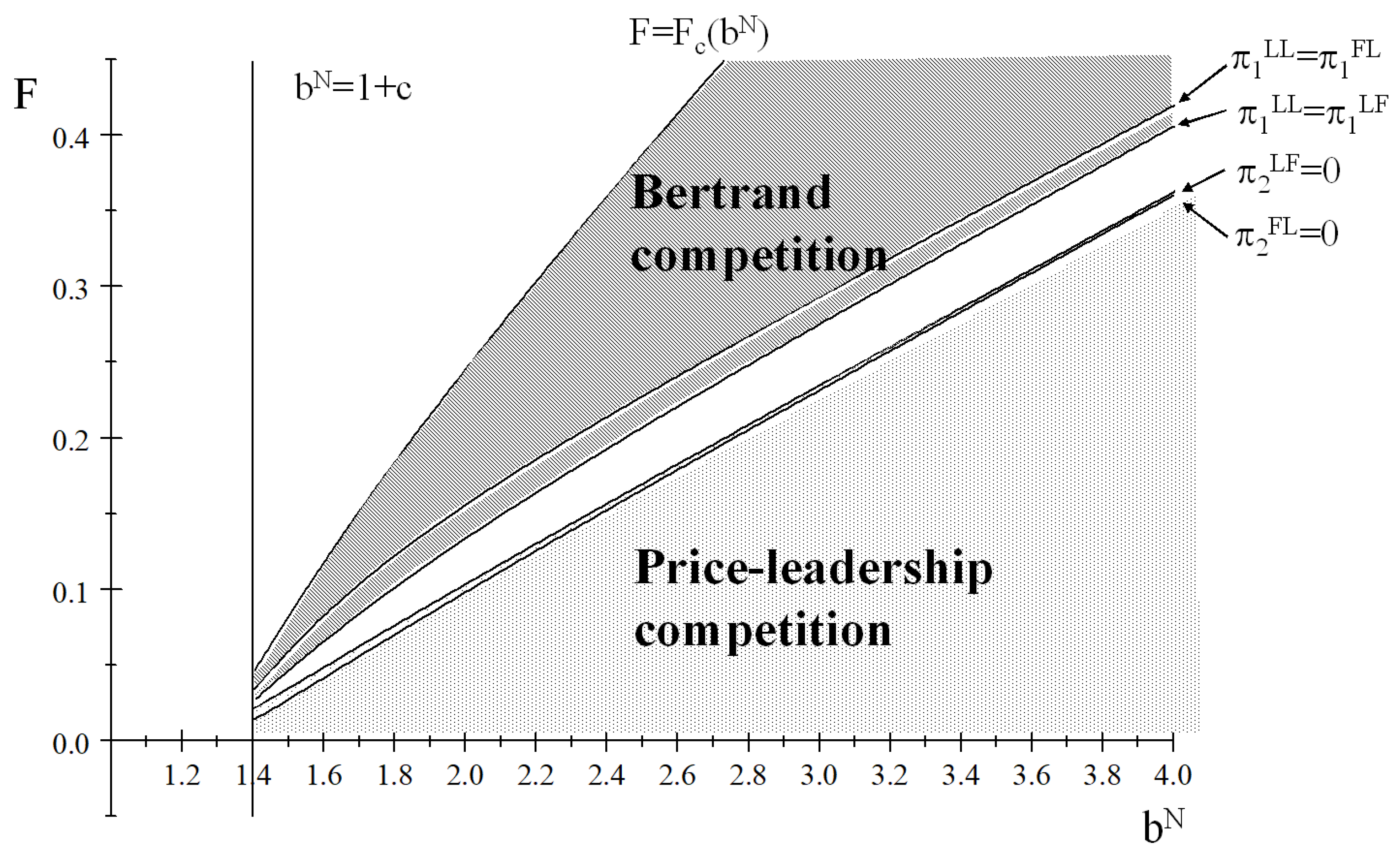
Theorem 2 states that the Bertrand price competition can emerge if the setup cost for producing new products is high enough. Both Theorems 2 and 3 can be understood intuitively by Figure 1, in which new and old products are sufficiently differentiated with respect to consumers’ willingness to pay. The figure depicts the relationship between $(b^N,F)$ and the type of competition in the range of $b^N\ge 1+c$ when $c=0.4.$

In the figure, ($b^N,F$) in the area between the lines $F=F_c(b^N)$ and ${\pi }_1^{LL}={\pi }_1^{LF}$ satisfies the Bertrand equilibrium, and ($b^N,F$) in the area between then lines ${\pi }_2^{LF}=0$ and $F=0$ ($b^N$-axis) satisfies the price-leadership equilibrium. From the figure, we can confirm that the theorems are true; that is, given $b^N$ and c, a higher F may induce the Bertrand equilibrium, while a lower F may induce the price-leadership equilibrium. In this study, we suppose that firms treat consumers’ willingness to pay for new products as given. Therefore, given a willingness to pay for new products, $b^N,$ the figure depicts the corresponding ranges of F where the Bertrand equilibrium emerges and where the price-leadership equilibrium does.

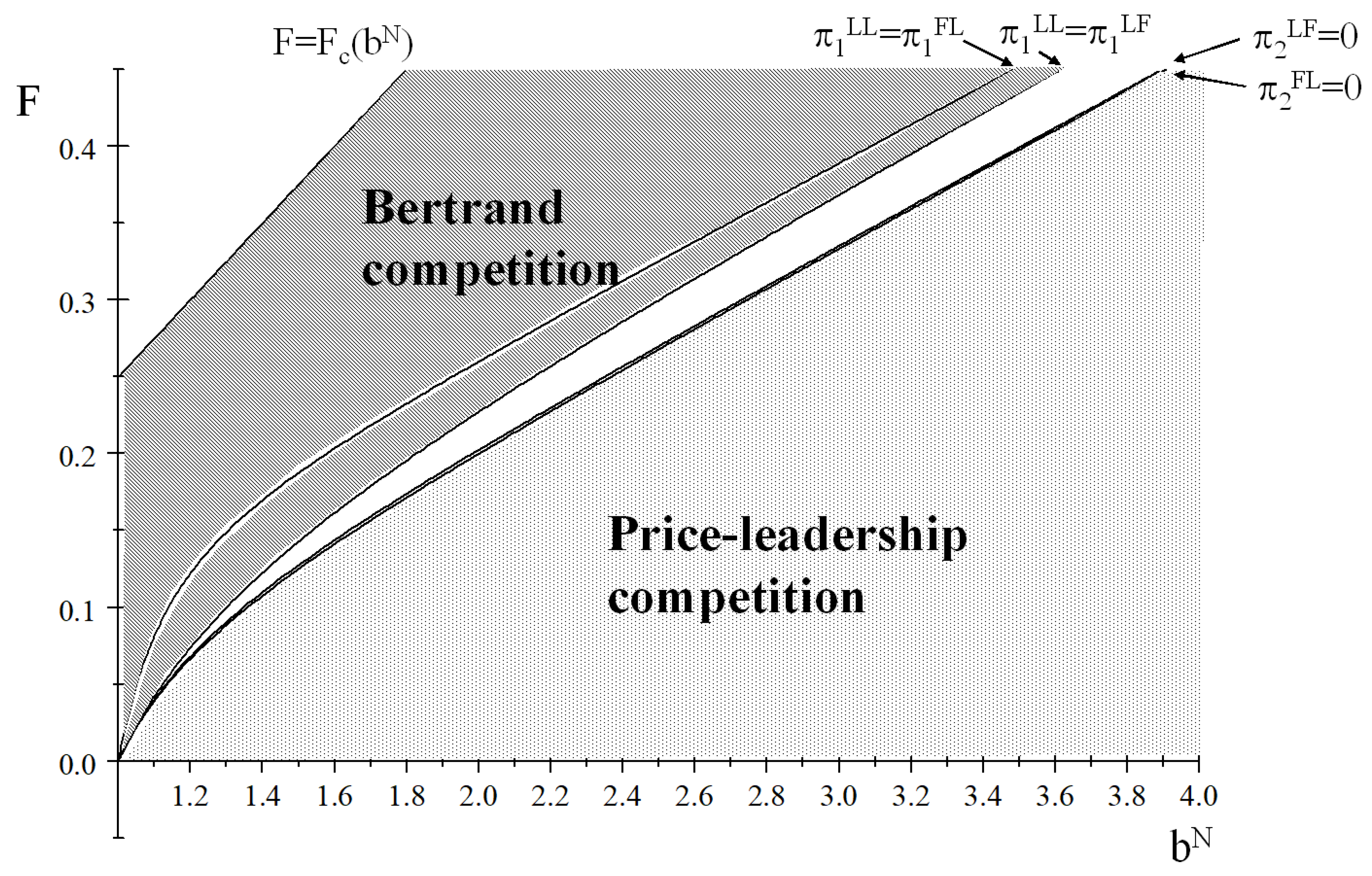
Figure 2 presents the relationship between the parameters ($b^N,F$) and the type of competition in the range of $b^N>1$ when $c=0.$ The relationship between the area ($b^N,F$) and the type of competition is the same as shown in Figure 1.

Both theorems indicate that the setup cost of producing the new product, $F,$ is a crucial factor in determining the type of competition in the product market. This finding is summarized as follows.

Proposition 1.

Consider the pricing strategy of duopolistic firms in the markets in which new and old products, substitutable and differentiated with respect to the willingness to pay, are supplied. If the setup cost of producing a new product is sufficiently high, Bertrand price competition emerges in the market for new products; otherwise, price-leadership competition can emerge in the market.

4. Discussion and Concluding Remarks

In a market where new products would replace existing ones, we often observe that firms engage in price competition. Despite this, little is known about the rationale behind the emergence of price competition in a new product market. Using an endogenous timing model with duopoly firms, this paper demonstrates that a setup cost for producing a new product plays an important role in determining the timing of pricing among the firms. In particular, we show that Bertrand price competition endogenously emerges when the setup cost is sufficiently high because under this condition, a firm can obtain a higher positive profit if it captures all the market demand by undercutting the price, which induces Bertrand price competition.

Our results have a policy implication such that government policies affecting the setup cost for a new product can change the type of competition in the new product market. In order to promote or protect new products in their domestic market, governments introduce economic policies in the form of subsidies, licensing for business operation, tariffs, and so on. This paper demonstrates that these policies change not only price or quantities but also type of competition under duopoly.

This implication is related with creation of high quality markets. For the healthy growth of a modern economy, high quality markets are indispensable (Yano [23]). It is because a market plays the role of a pipe that connects new technologies to people’s live (See Dastidar [24]). Recent literature on market quality theory includes Furukawa and Yano [25], Wang and Ota [26], Yano [27], and Dastidar and Yano [28]. This implies that the high quality market will give many consumers easy access to new products, which are often embodied by state-of-the-art technologies, and as result improve both consumer surplus and producer surplus. If so, competitive price is essential, that is, type of competition matters for market quality. Our finding suggests that the market quality may be enhanced by government policies changing the setup cost for the new product, by which the type of competition can change.

This paper investigates endogenous emergence of competition type under duopoly. However, there will be potential firms consider entering or exiting the new product market depending on the type of competition. For example, under Stackelberg competition, Etro [29] allows free entry and exit and studies endogenous market structure. Policy implications from the model cover the wide range of aspects including industrial organization, international trade, and economic growth, although that study does not analyze endogenous emergence of competition type (See Etro [30] for policy implications). A promising future work is an integration of our model and the model of endogenous market structure. This will bring deeper understanding on the formation of competition type.