Comparing Bayesian Spatial Conditional Overdispersion and the Besag–York–Mollié Models: Application to Infant Mortality Rates

Abstract

In this paper, we review overdispersed Bayesian generalized spatial conditional count data models. Their usefulness is illustrated with their application to infant mortality rates from Colombian regions and by comparing them with the widely used Besag–York–Mollié (BYM) models. These overdispersed models assume that excess of dispersion in the data may be partially caused from the possible spatial dependence existing among the different spatial units. Thus, specific regression structures are then proposed both for the conditional mean and for the dispersion parameter in the models, including covariates, as well as an assumed spatial neighborhood structure. We focus on the case of response variables following a Poisson distribution, specifically concentrating on the spatial generalized conditional normal overdispersion Poisson model. Models were fitted by making use of the Markov Chain Monte Carlo (MCMC) and Integrated Nested Laplace Approximation (INLA) algorithms in the specific context of Bayesian estimation methods.

1. Introduction

Generalized linear models (GLM) are commonly used to model the response variable when working with count data (see [1]). However, count data regression models commonly exhibit overdispersion, a phenomenon generated when the data show a larger variance than the one that would be expected from the specification of the model itself (see [2]). This situation is also known as extra-Poisson or extra-binomial variation when the response variable is assumed to follow either a Poisson or a binomial distribution, respectively. Fitting a model without taking into account the presence of overdispersion may result in standard errors underestimation, among other problems, which can lead to an inferential process that may be incorrect (see [2]). One of the possible causes for overdispersion is the presence of correlation among the values of the variable under study for the different units considered in the specific data set being analyzed (see [3]). This is specially common with spatial data, where observations in locations that are closer in space tend to show similar values, a phenomenon known as spatial autocorrelation (see [4]). Consequently, these issues must be taken into account in order to obtain reliable inference processes for the estimated parameters in the proposed model.

Overdispersion has been extensively studied in the literature, particularly for the case of response variables which follow a Poisson or a binomial distribution. A common way to deal with overdispersion in these cases is to modify the mean variance relation for the model by scaling it with a dispersion parameter larger than one, and then use a quasi-likelihood approach for the estimation (see [1]). For overdispersed count data following a Poisson distribution, perhaps the most popular model is the negative binomial model, initially proposed by Margolin, Kaplan and Zeiger [5], who applied their proposed model to data from a mutagenicity assay for the Salmonella bacteria. They were able to model the variability and, hence, the precision, when replicating plate environments by means of the extra-Poisson variation parameter. The normal or log-normal Poisson models, proposed by Hinde [3], included a random effect following a normal distribution in the linear predictor, with a variance given by the extra parameter, so that it allowed for the possible existing overdispersion in the model specification itself. This model has been used for the analysis of cancer death rates by Breslow [6], where he proposed two estimation methods by weighted least squares in three steps. Results indicated that there was a clear evidence of variability in the data that the Poisson model failed to capture, an issue that was resolved with the fitting of the normal Poisson model with the extra overdispersion parameter included in it.

Williams [7] proposed the beta-binomial model for the case of binomial responses. This model assumed that the probability of success from the binomial distribution is a random variable following a beta distribution, which includes an additional parameter to model the extra-binomial variation. Williams [8] also modified the logistic linear model by incorporating an extra-binomial variation component and proposed a methodology for computing the maximum likelihood estimates of the regression parameters based on iterated re-weighted least squares. He applied his proposal to a data set where it was required to model the proportion of germinating seeds of two different types and root extracts, finding similar results when comparing his model’s estimates to those from other models previously proposed in the literature. The normal binomial model can be obtained as an extension of this model by considering that the extra-binomial variation component follows a normal distribution (see [9]).

Most overdispersion models assume the existence of constant dispersion in the data but, in a considerable number of cases, dispersion could behave differently. Therefore, models have been developed to allow for the dispersion to vary as a function of some explanatory variables. Hinde and Demétrio [2] and McCullagh and Nelder [1] mentioned the idea of joint modeling of the mean and dispersion parameters. Double exponential families were introduced and applied to specific settings for the binomial and Poisson cases by Efron [10]. These distributions allow to model the mean of exponential family distributions, as well as to be able to capture the possible existing overdispersion in count data by specifying a regression model for the dispersion parameter. Quintero-Sarmiento, Cepeda-Cuervo and Núñez-Antón [9] proposed Bayesian extensions of overdispersion models, such as the negative binomial and the normal Poisson models for count data, where they assumed regression structures both for the mean and for the dispersion parameters, and, therefore, they were able to specify the so-called generalized overdispersion models.

Two of the most common model specifications to account for spatial dependence in the data are the Conditional Autoregressive (CAR) model [11] and the Simultaneous Autoregressive (SAR) model [12]. These models incorporate the spatial correlation by assuming a conditional covariance structure specified by means of a spatial neighborhood matrix. Wall [13] examined the correlation structures that these models imply in detail by fitting them to SAT scores from students in the USA, which led to finding conterintuitive results given that the assumed CAR and SAR structures for this data implied spatial correlations among some states that did not correspond to reality or to the specific data set characteristics.

Besag [11] introduced autoregressive models for count data, such as the auto-binomial and auto-Poisson models, among others, by following the SAR model’s structure. These models, however, present the disadvantage that they can only account for negative spatial autocorrelation in the data (see [14]). The spatial autoregressive Poisson model was proposed by Lambert, Brown and Florax [15], who assumed a SAR model’s structure for the mean of the response variable, for which a two step limited information maximum likelihood estimation method was also proposed. They analyzed a data set concerning firm births in the different states in the USA for the period 2000–2004, and concluded that this proposed model and estimation method allowed them to better understand how geographical determinants can affect the firm births under study.

In the context of Bayesian regression models for count data, spatial dependence is commonly addressed by specifying a hierarchical model, including a set of random effects in the linear predictor of a GLM, for which spatially correlated prior distributions are usually assumed. In this way, the CAR model’s structure has been extended by the well known Besag–York–Mollié (BYM) model (see [16]), where the spatial dependence in the data is incorporated by means of a spatially correlated prior with intrinsic CAR distribution, and an extra-variability is also included with a set of uncorrelated random effects. This model, in particular, is widely used for estimating relative risks in small areas in disease mapping (see [17]). Comparison between this model and alternative models applied in this area can be found in Best, Richardson and Thomson [18]. Alternative variants of prior distributions that have been proposed can be also consulted in Lee [19].

More recently, a new parameterization of the BYM model has been developed with the proposal of the so-called BYM2 model, which allows for a more comprehensible interpretation of the parameters and offers some other improvements over the BYM model (see [20]). Morris, Wheeler-Martin, Simpson, Mooney, Gelman and DiMaggio [21] applied the BYM2 model to a data set of motor vehicle crashes from 2005 to 2014, where school-age pedestrians resulted injured in the city of New York, and explored sociodemographic factors related to their occurrence. They concluded that the BYM2 model offered a good fit to this data and are able to identify areas with increased risk of pedestrian injuries in crashes, and to establish positive relationships between this risk and the number of people who commute to work via walking, bicycle and public transport.

In order to be able to address the issue of spatial autocorrelation in the data, Cepeda-Cuervo, Córdoba and Núñez-Antón [22] proposed the spatial conditional models for overdispersed spatial count data, where they assumed that part of the overdispersion can be explained by the spatial neighborhood structure in the proposed models. This model accounts for the spatial dependence in the data by incorporating a spatial term in the linear predictor with a parameter that estimates the intensity of the spatial association. By adopting a Bayesian framework, the authors applied these models to infant mortality data from Colombia and to postnatal screening tests, obtaining good fit and being able to model the positive spatial dependence, as well as accounting for data overdispersion. Additionally, to allow for nonconstant overdispersion, extensions of the generalized overdispersion models of Quintero-Sarmiento, Cepeda-Cuervo and Núñez-Antón [9] were also proposed by incorporating spatial neighborhood structures in the regressions for the mean and the variance and, thus, proposing the so-called generalized spatial conditional overdispersion models.

When fitting Bayesian models, it is not always possible to obtain analytically closed form expressions for the posterior distribution (see [23]). Therefore, it is necessary to approximate this distribution by computational methods. One of the most extended examples of these approximation methods is the Markov Chain Monte Carlo (MCMC) approach, an algorithm that generates simulated samples from the posterior distributions of the regression parameters by the Gibbs sampling method, a special case of the Metropolis–Hastings algorithm (see [23,24,25]). An alternative to computational algorithms, such as the MCMC methods in the Bayesian estimation mentioned above, is the Integrated Nested Laplace Approximation (INLA) algorithm (see [26]), which is based on the deterministic numerical computation of posterior distributions approximations.

There are several software packages available for the estimation of Bayesian models, such as, for example, OpenBUGS [27] and the CARBayes R package [19], both using the MCMC approach and, the R-INLA R package [28], which uses the INLA approach. Carroll, Lawson, Faes, Kirby, Aregay and Watjou [29] studied models to account for spatial dependence for Poisson distributed count data in disease mapping, and their performance is compared for the two software packages OpenBUGS and R-INLA. More specifically, the authors fitted some models such as the Poisson, normal Poisson and BYM models, among others, to simulated count data for which spatial correlation structures were implemented in different ways. Reported results concluded that there were substantial differences in the two implementations, especially for the estimation of the random effects, but they managed to find a good fit in both cases by varying some of the prior settings. Moreover, they highlighted the much shorter computation time that R-INLA required for the fitting of a model when compared to OpenBUGS. In Vranckx, Neyens and Faes [30], an extensive comparison of the fitting of the BYM model with OpenBUGS, CARBayes, R-INLA and other available software packages was also reported by fitting data from young people receiving diabetes medication in Belgian municipalities for the year 2014. Although no covariates were used in their analysis, the authors were able to identify locations with increased relative risk by fitting the BYM model to the data set under study.

The main objective of this paper was to review regression models for spatial count data with overdispersion, such as the spatial conditional overdispersion models and the BYM models, and to be able to provide a comparison between the performance of both models, particularly focusing on the case where the response variable follows a Poisson distribution. In Section 2, we describe the models to be fitted and explain the methods that will be used for their estimation within a Bayesian context. In Section 3, we provide an application of these models to infant mortality rates from Colombia and present the most relevant results. Section 4 concludes with a brief discussion on the findings.

2. Methods and Models

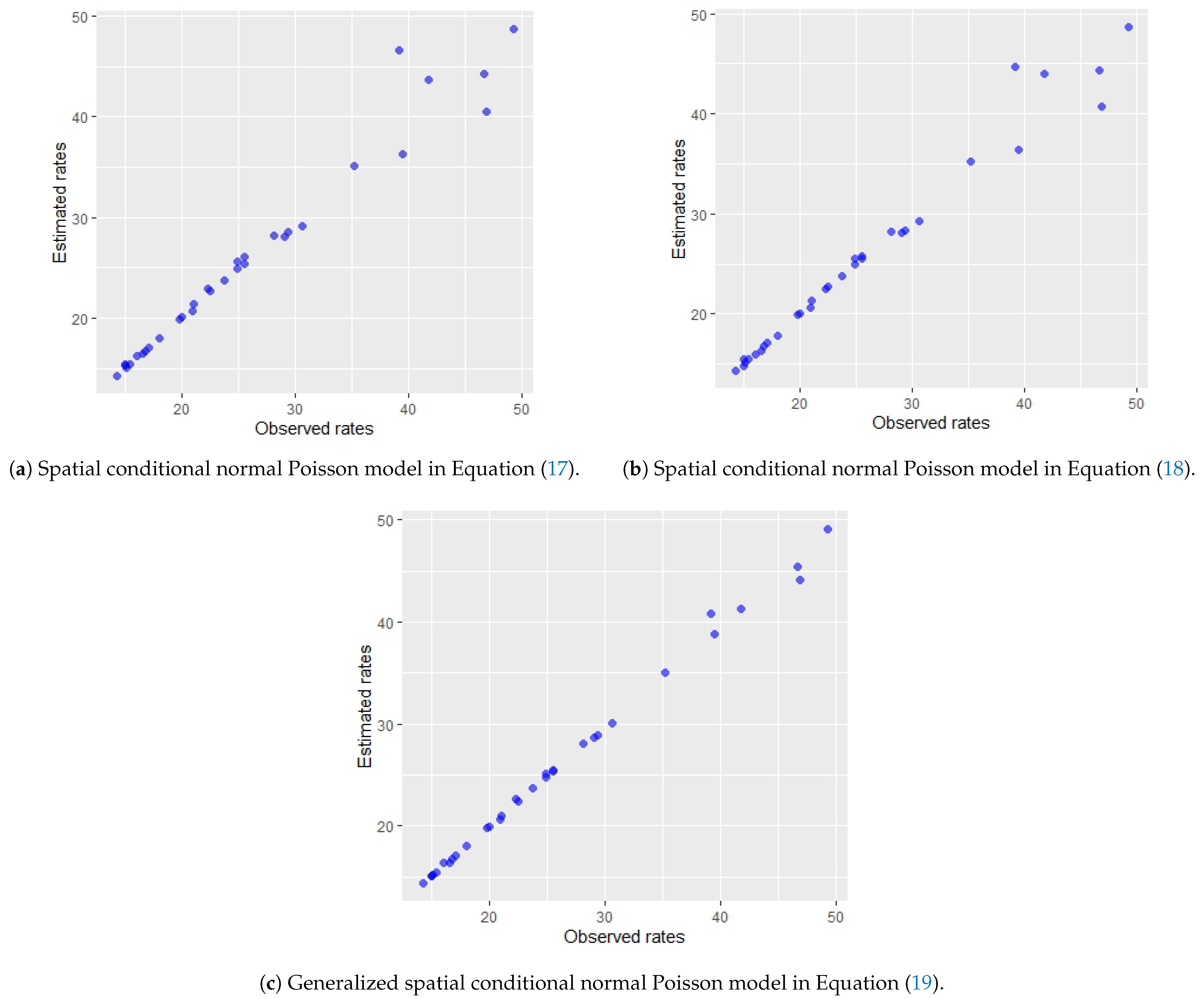
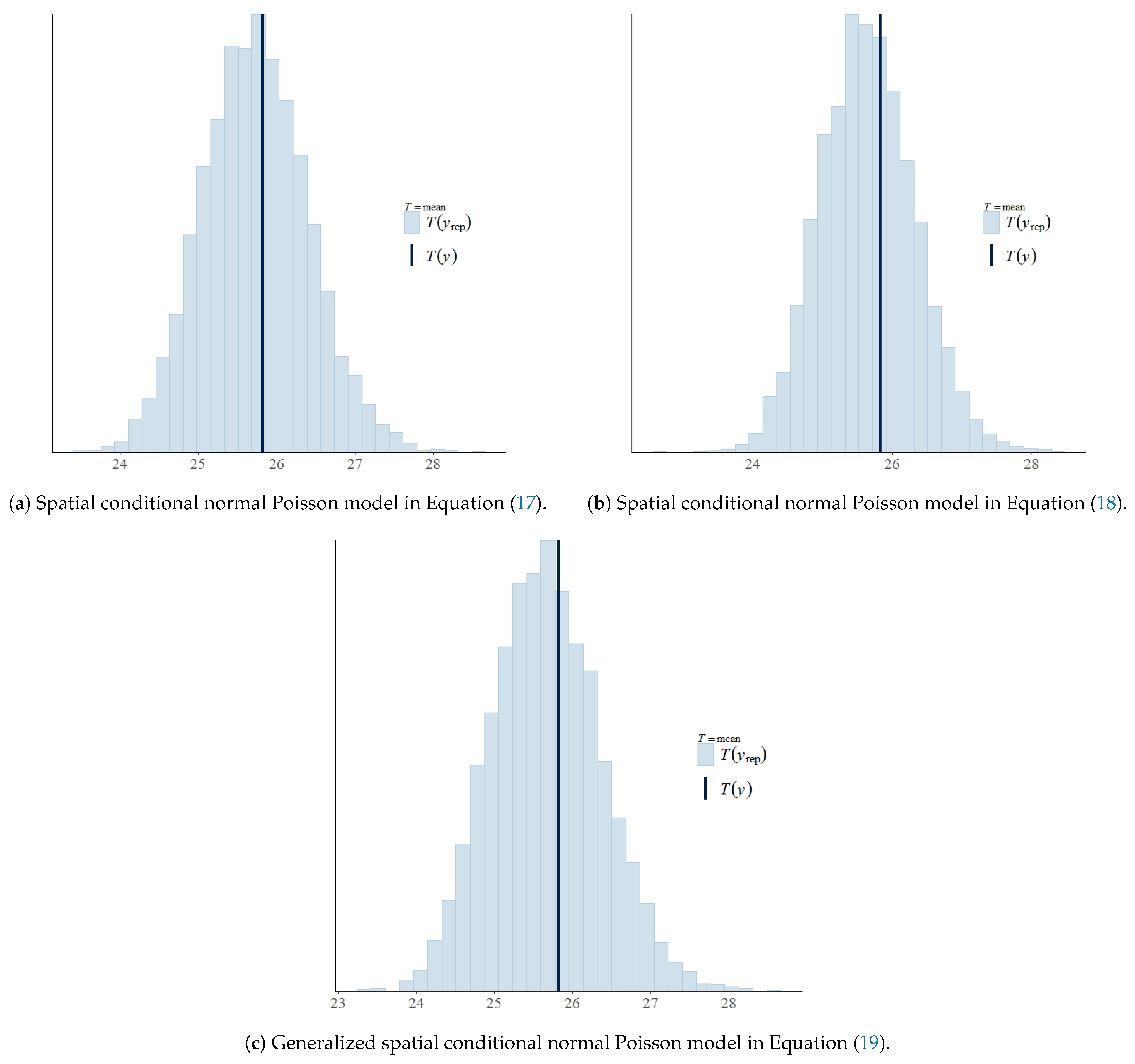
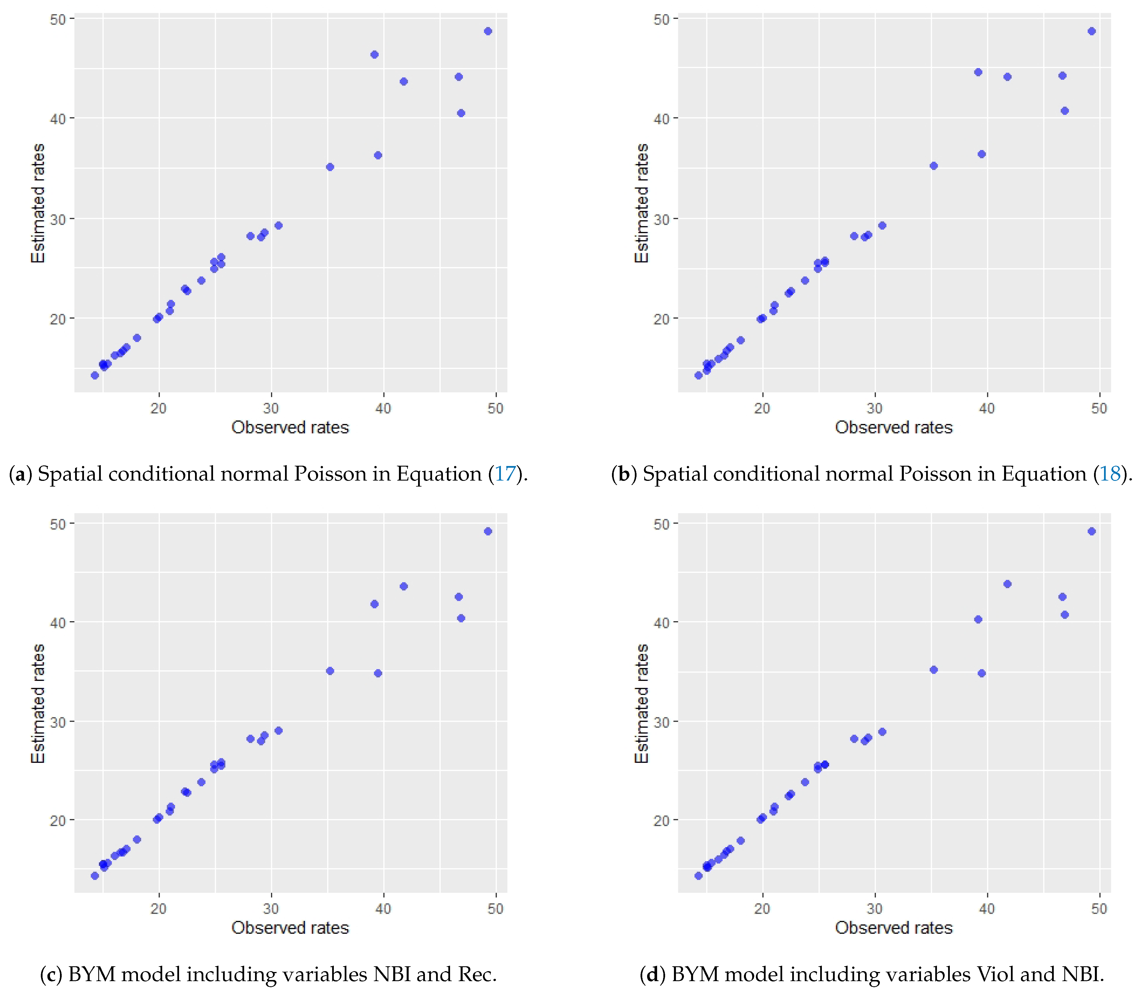
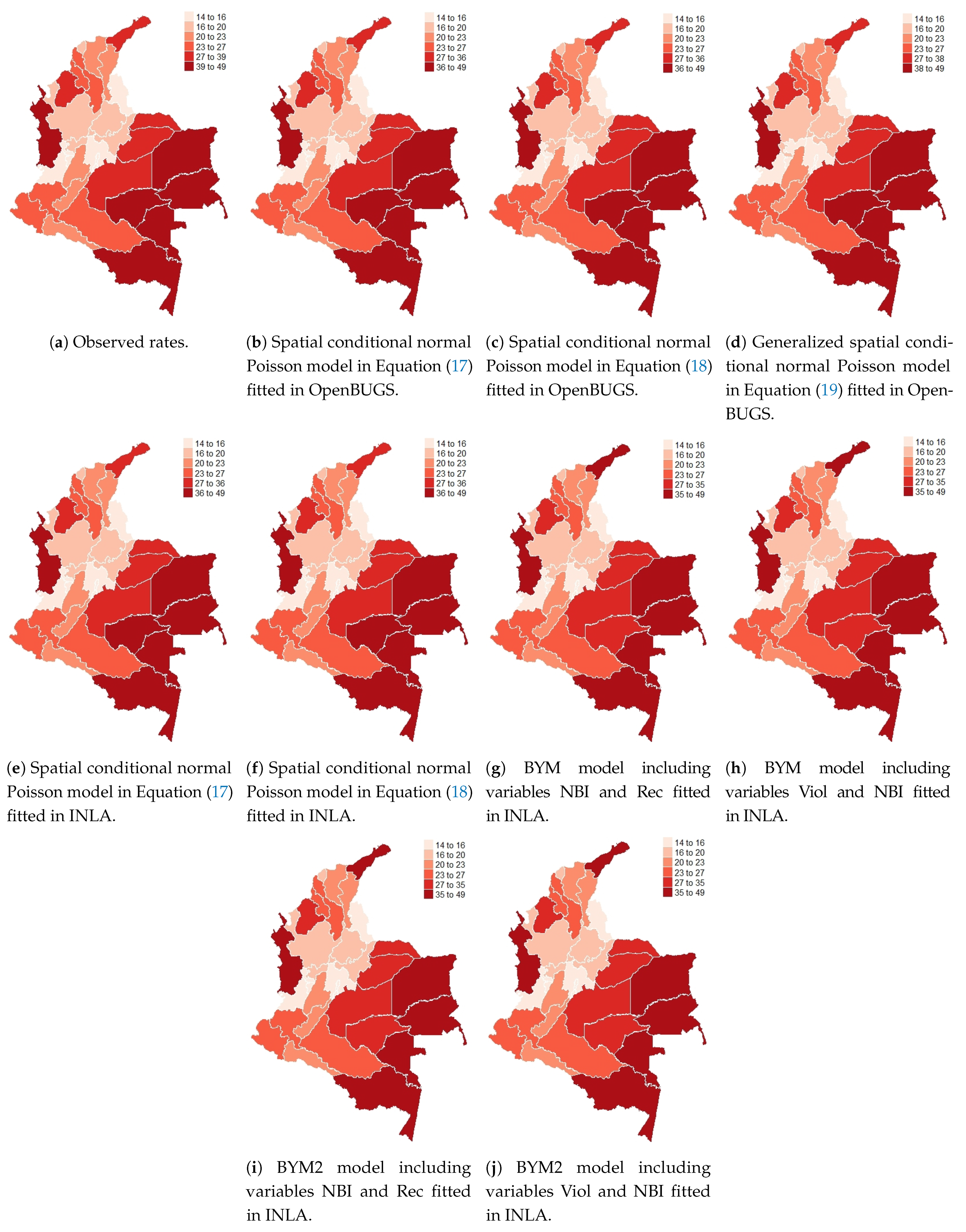
2.1. Spatial Conditional Overdispersion Models

Let us suppose that the random variables $Y_i$, for $i=1,\cdots ,n$, represent counts with corresponding means $\mathrm{E}\left(Y_i\right)={\mu }_i$. The Poisson model generally assumes that $Y_i\sim \mathrm{Poi}\left({\mu }_i\right)$, with variance $\mathrm{Var}\left(Y_i\right)={\mu }_i$, so that the variance is equal to the mean, a property that is known as equidispersion. In a generalized linear model, the mean of the distribution depends on the explanatory variables through the following regression model, known as linear predictor:

$$g\left(\mu \right)={\mathbf{x}}_i^T\mathit{\beta },$$

(1)

where $g(.)$ is a monotonic and differentiable link function, ${\mathbf{x}}_i$ is the $k\times 1$ vector of explanatory variables for the i-th observation and $\mathit{\beta }$ is the $k\times 1$ vector of unknown regression parameters that need to be estimated. For the Poisson regression model, the natural logarithm is often chosen as the link function; that is, $g\left(\mu \right)=log\left(\mu \right)$. Under these assumptions, overdispersion would occur when there is extra-Poisson variability in the data, so that $\mathrm{Var}\left(Y_i\right)>{\mu }_i$.

Two of the most common models used to accommodate overdispersion in count data for the case of response variables following a Poisson distribution are the normal Poisson and the negative binomial models. In the normal Poisson model, the overdispersion is corrected by the inclusion of a random effect, assumed to be normally distributed, in the linear predictor. In this way, the normal Poisson can be written as:

$$log\left({\mu }_i\right)={\mathbf{x}}_i^T\mathit{\beta }+{\nu }_i,$$

(2)

where ${\mathbf{x}}_i$ and $\mathit{\beta }$ are as before, and ${\nu }_i\sim N(0,\tau )$, for $i=1,\cdots ,n$. In this model, $\left(Y_i\right|{\nu }_i)$, for $i=1,\cdots ,n$, follows a Poisson distribution with conditional mean $\mathrm{E}\left(Y_i\right|{\nu }_i)={\mu }_i$. Although the distribution of $Y_i$ does not have a closed form expression (see [3]), when the variance $\tau$ of the random effects is small enough, the random variables $Y_i,i=1,\cdots ,n$, can be considered as mixed Poisson variables, with mean and variance that can be approximated by $\mathrm{E}\left(Y_i\right)\approx {\mu }_i$ and $\mathrm{V}ar\left(Y_i\right)\approx {\mu }_i+\tau {\mu }_i^2$ (see [31]). The dispersion parameter $\tau$ allows for modeling the possible existing overdispersion and, in addition, it also captures the variability unexplained by the covariates. That is, since $\tau >0$, the variance is larger than that specified by the Poisson model, so that ${\mu }_i+\tau {\mu }_i^2>{\mu }_i$. We believe it is important to mention that the condition that the variance $\tau$ of the random effects should be small enough (see [3] or [31]) is satisfied in the relevant cases in the application of this model in Section 3, so that the approximations mentioned above hold.

Another frequently used model to fit overdispersed count data is the standard negative binomial or NB2 model (see [32]). One possible way to be able to generate this model is by considering a Poisson-gamma mixture. That is, if we assume that the random variables $m_i,i=1,\cdots ,n$, follow a Gamma distribution, such that $m_i\sim G(\tau ,\tau )$, with $\tau >0$ a parameter that needs to be estimated, and that the random count variables $Y_i,i=1,\cdots ,n$, conditioned on ${\mu }_i$ and the random variables $m_i$ follow a Poisson distribution with mean $\mathrm{E}\left(Y_i\right)={\mu }_i{m}_i$, such that $Y_i\sim \mathrm{Poi}\left({\mu }_i{m}_i\right)$, then the unconditional distribution of $Y_i$ can be derived in the following way [32]:

$$f(y_i)={\int }_0^{\infty }f(y_i|m_i)f\left(m_i\right)d{m}_i=\left(\genfrac{}{}{0pt}{}{y_i+\tau -1}{y_i}\right){\left({\displaystyle \frac{\tau }{\tau +{\mu }_i}}\right)}^{\tau }{\left({\displaystyle \frac{{\mu }_i}{\tau +{\mu }_i}}\right)}^{y_i},$$

(3)

which corresponds to the probability density for a negative binomial distributed count variable, so that $Y_i\sim \mathrm{NB}(\tau /(\tau +{\mu }_i),\tau ),i=1,\cdots ,n$, with mean $\mathrm{E}\left(Y_i\right)={\mu }_i$ and variance $\mathrm{Var}\left(Y_i\right)={\mu }_i+{\tau }^{-1}{\mu }_i^2$. The dispersion parameter $\tau$ allows for the modeling of the extra-Poisson variability because, since we have that $\tau >0$, then ${\mu }_i+{\tau }^{-1}{\mu }_i^2>{\mu }_i$. Therefore, and from the above, for the negative binomial regression model, the linear predictor is specified for the mean ${\mu }_i$, so that:

$$log\left({\mu }_i\right)={\mathbf{x}}_i^T\mathit{\beta },$$

(4)

where ${\mathbf{x}}_i$ and $\mathit{\beta }$ are as above.

One of the reasons for the existence of overdispersion in spatial data may be the possibly existing spatial correlation between the responses corresponding to the different adjacent locations. Hence, it can be assumed that a portion of the overdispersion can be explained by taking into account this spatial correlation. Thus, the spatial conditional overdispersion regression models proposed by Cepeda-Cuervo, Córdoba and Núñez-Antón [22] assumed a specific spatial structure for the variable under study. That is, they assumed that $Y_i$, for $i=1,\cdots ,n$, conditioned on the values in all of the neighbors of the ith region, except for the i-th region itself (i.e., $Y_{\sim i}$), follows a conditional overdispersed distribution denoted by $f\left(y_i\right|y_{\sim i})$, for $i=1,\cdots ,n$. In this distribution, the conditional mean follows a given regression structure that includes some covariates affecting the response variable, as well as its spatial lags, together with a spatial parameter that allows to account for the intensity of the spatial dependence that is present in the data. In the case where the conditional distribution follows one of the aforementioned models, this model leads to the spatial conditional Poisson, negative binomial and normal Poisson regression models, respectively.

The spatial distribution is commonly specified by means of a neighborhood structure, defined, for a sample of n regions, by an $n\times n$ spatial weights matrix, denoted by $\mathbf{W}=\left[w_{ij}\right]$, where its elements, $w_{ij}$, are the weights to be specifically used to model the strength of the dependence between the i-th and the j-th regions. These elements are given by the contiguity criteria chosen by the researcher, which can be based on the boundaries of the regions or on the distance from one spatial location to the others, or by any other alternative criteria previously proposed in the literature. It is commonly assumed that, $w_{ij}=1$, if region i is adjacent or a neighbor to region j, and $w_{ij}=0$, otherwise. First order contiguity can be specified, for example, when we use the criteria that regions i and j are neighbors if they share at least one point in their boundaries. Second order could also be considered if we extend the criteria by considering that i and j are neighbors if they share a common neighbor. This weights matrix is usually standardized by rows, so that, if region i is adjacent to region j, then $w_{ij}=1/n_i$, where $n_i$ is the number of neighbors region i has. Along these lines, if $\mathbf{y}$ is the $n\times 1$ vector of observations for a response variable Y, then the spatial lag of Y is defined as the product of the $1\times n$ vector corresponding to the ith row of the weights matrix $\mathbf{W}$, ${\mathbf{W}}_i$, and the vector $\mathbf{y}$; that is, ${\mathbf{W}}_i\mathbf{y}$, a product representing the averaged values of the considered variable in the neighboring locations for the ith region. In this work, we only assume first order adjacency among regions and, in addition, that the spatial weights matrix is standardized by rows.

The spatial conditional Poisson model is specified by assuming that the conditional distribution of the variable under study follows a Poisson distribution, that is $\left(Y_i\right|Y_{\sim i})\sim \mathrm{Poi}\left({\mu }_i\right)$, with conditional mean $\mathrm{E}\left(Y_i\right|Y_{\sim i})={\mu }_i$, so that its corresponding regression model, where the previously described spatial association dependence is incorporated, can be specified as:

$$log\left({\mu }_i\right)={\mathbf{x}}_i^T\mathit{\beta }+\rho {\mathbf{W}}_i\mathbf{y},$$

(5)

where ${\mathbf{x}}_i$ and $\mathit{\beta }$ are as above, $\rho$ is the parameter incorporating the first order spatial association, ${\mathbf{W}}_i$ is the ith row of the $n\times n$ weight matrix $\mathbf{W}$ that represents the spatial neighborhood structure assumed in the model, and $\mathbf{y}$ is the vector of dimension $n\times 1$ for the observed values for the response variable under study.

The spatial conditional normal Poisson model assumes that the distribution of the variable under study, conditioned on its neighbors excluding the i-region itself, $Y_{\sim i}$, and the normally distributed random effect ${\nu }_i\sim N(0,\tau )$, follows a Poisson distribution. That is, $\left(Y_i\right|Y_{\sim i},{\nu }_i)\sim \mathrm{Poi}\left({\mu }_i\right)$, with conditional mean $\mathrm{E}\left(Y_i\right|Y_{\sim i},{\nu }_i)={\mu }_i$, so that its corresponding regression model, where the previously described spatial association dependence is incorporated, can be specified as:

$$log\left({\mu }_i\right)={\mathbf{x}}_i^T\mathit{\beta }+\rho {\mathbf{W}}_i\mathbf{y}+{\nu }_i,$$

(6)

where ${\mathbf{x}}_i$, $\mathit{\beta }$, $\rho$, ${\mathbf{W}}_i$ and $\mathbf{y}$ are as above.

In the same way, the spatial conditional negative binomial model can be also specified if we assume that the response variable under study, conditioned on $Y_{\sim i}$, follows a negative binomial distribution. That is, $\left(Y_i\right|Y_{\sim i})\sim \mathrm{NB}(\tau /(\tau +{\mu }_i),\tau )$, with conditional mean $\mathrm{E}\left(Y_i\right|Y_{\sim i})={\mu }_i$, and with a regression structure given by Equation (5).

We believe it is important to mention that, in the spatial conditional normal Poisson and the spatial conditional negative binomial models, a portion of the overdispersion that may have been generated by the possible existing spatial correlation in the data is considered to be incorporated into the model by using the specified neighborhood spatial structure, given by the product between the spatial weights matrix and the vector of responses (i.e., by incorporating spatial lags of the variable under study), ${\mathbf{W}}_i\mathbf{y}$. The remaining unexplained overdispersion in the data will be modeled by means of the dispersion parameter $\tau$. However, we should note that these models assume a constant overdispersion, and there are cases where the dispersion in the data can vary among groups or observations. The generalized overdispersion models proposed by Quintero-Sarmiento, Cepeda-Cuervo and Núñez-Antón [9] introduced Bayesian extensions of the standard overdispersion models, where regression structures are assumed both for the mean and for the dispersion parameter. Their model allowed for the dispersion to vary as a function of some explanatory variables, so that dispersion can vary for the different regions or observations in the study.

In this sense, generalized overdispersion models offer a reasonable and well justified proposal for fitting count data with overdispersion. However, for the case of spatial count data, they do not provide information or incorporate into the model the possible existing spatial dependence in the data set under study, which clearly motivates the inclusion of the spatial dependence structure in these models. Along these lines, the generalized spatial conditional overdispersion regression models [22] assumed that the spatial count variable in their model, $Y_i,i=1,\cdots ,n$, conditioned on the values in all of the neighbors of it, except for the ith region itself (i.e., $Y_{\sim i}$), follows an overdispersed conditional distribution $f\left(y_i\right|y_{\sim i}),i=1,\cdots ,n$, with conditional mean and dispersion parameter following specific regression structures that include some covariates affecting the response variable and the spatial lags of the variable of interest.

If we now consider the case where $Y_i$ follows a Poisson distribution with mean ${\mu }_i$, and assume the normal Poisson model with mean structure given by Equation (6), for the generalized spatial conditional normal Poisson model, we will have that the conditional mean and variance components in the random effect distribution will be specified by regression structures given by:

$$log\left({\mu }_i\right)={\mathbf{X}}_i^T\mathit{\beta }+{\rho }_1{\mathbf{W}}_i\mathbf{y}+{\nu }_i\mathrm{and}log\left({\tau }_i\right)={\mathbf{Z}}_i^T\mathbf{\gamma }+{\rho }_2{\mathbf{W}}_i\mathbf{y},$$

(7)

where ${\mathbf{x}}_i$, $\mathit{\beta }$, ${\mathbf{W}}_i$ and $\mathbf{y}$ are as above, and ${\rho }_1$ and ${\rho }_2$ are the parameters that explain the spatial association in the mean and dispersion structures, respectively. In addition, ${\mathbf{Z}}_i$ is the $q\times 1$ vector of explanatory variables for the ith observation and $\mathbf{\gamma }$ is a vector of dimension $q\times 1$ containing the unknown regression parameters that need to be estimated. The generalized spatial conditional negative binomial model can be specified in the same way, by assuming that $Y_i,i=1,\cdots ,n$, conditioned on $Y_{\sim i}$, follows a negative binomial distribution, and assuming the following regression structures for both the conditional mean and dispersion parameter:

$$log\left({\mu }_i\right)={\mathbf{X}}_i^T\mathit{\beta }+{\rho }_1{\mathbf{W}}_i\mathbf{y}\mathrm{and}log\left({\tau }_i\right)={\mathbf{Z}}_i^T\mathbf{\gamma }+{\rho }_2{\mathbf{W}}_i\mathbf{y},$$

(8)

where ${\mathbf{x}}_i$, $\mathit{\beta }$, ${\mathbf{W}}_i$, $\mathbf{y}$, ${\rho }_1$, ${\rho }_2$, ${\mathbf{Z}}_i$ and $\mathbf{\gamma }$ are as above.

2.2. Besag–York–Mollié (BYM) Model

The Besag–York–Mollié (BYM) model [16] is a Bayesian Poisson hierarchical model widely used in the literature for fitting spatial count data, particularly in the field of disease mapping (see [17]). It is an extension of the generalized linear Poisson model that includes both a spatial structured and an unstructured random effect in the regression model structure. If we let $Y_i,i=1,\cdots ,n$ represent counts for the n different regions, the BYM model is specified by assuming that the variable under study follows a Poisson distribution with mean $\mathrm{E}\left(Y_i\right)={\mu }_i$, having a mean regression structure given by:

$$log\left({\mu }_i\right)={\mathbf{x}}_i^T\mathit{\beta }+{\nu }_i+{\eta }_i,$$

(9)

where ${\mathbf{x}}_i$ and $\mathit{\beta }$ are as above, ${\nu }_i$ is a normally distributed random effect, so that ${\nu }_i\sim N(0,\tau )$, with $\tau >0$ being an unknown variance parameter that needs to be estimated, and ${\eta }_i$ is an intrinsic conditional autoregressive (CAR) [16] distributed random effect, so that:

$$\left({\eta }_i\right|{\eta }_{\sim i},\mathbf{W},{\tau }_{\eta })\sim N\left(\frac{{\sum }_{j=1}^N{w}_{ij}{\eta }_j}{{\sum }_{j=1}^N{w}_{ij}},\frac{{\tau }_{\eta }}{{\sum }_{j=1}^N{w}_{ij}}\right),$$

(10)

where ${\eta }_{\sim i}$ represents the set of values of all neighbors of the ith region, except for the ith region itself, $\mathbf{W}$ is the spatial weights matrix and ${\tau }_{\eta }$ is an unknown variance parameter that needs to be estimated. Given that this model is able to account for spatial dependence and also for the extra-variability in the data set not explained by the covariates, it has a considerable potential to motivate and justify its use for the analysis of spatial count data. However, since it is only possible to obtain information from the data from the sum of the two random effects, but not from each of the individual components separately, its use in this specific context has been questioned because of the possible identifiability problems that it may present (see [33]).

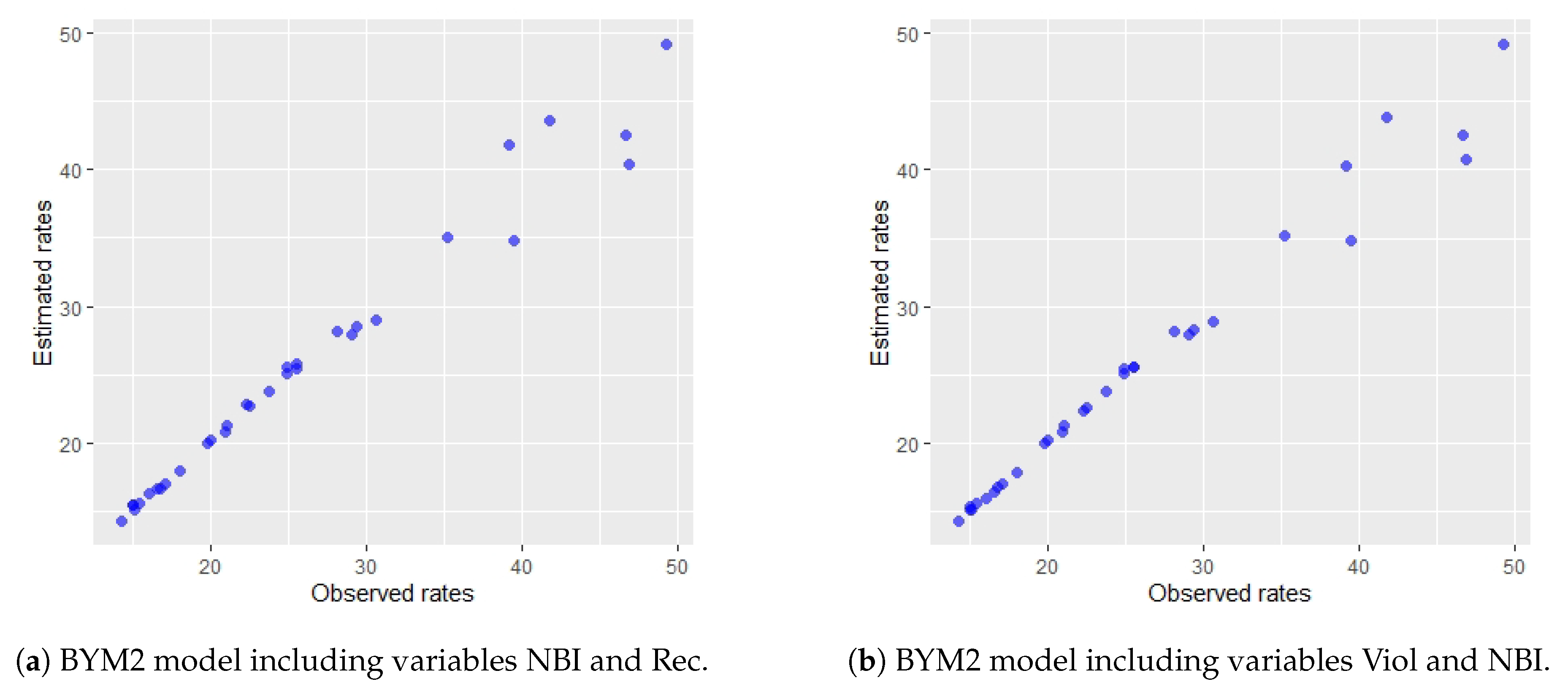
Some authors (e.g., Riebler, Sørbye, Simpson and Rue [20]) have addressed the issue of identifiability. They proposed the BYM2 model, an extension of the BYM model that scales the spatial component and the unstructured component, so that the mean regression structure can be written as:

$$log\left({\mu }_i\right)={\mathbf{x}}_i^T\mathit{\beta }+\frac{1}{\sqrt{{\tau }_s}}\left(\sqrt{1-{\varphi }_s}{\nu }_i+\sqrt{{\varphi }_s}{\eta }_i\right),$$

(11)

where the random effects ${\nu }_i$ and ${\eta }_i$ are as in the BYM model, but with a scaled variance approximately equal to one, ${\tau }_s$ is an unknown precision parameter that captures the variance contribution from the sum of the two random effects, and ${\varphi }_s$ is a mixing parameter that controls for the variance contribution of the spatially structured component $\eta ={({\eta }_1,\cdots ,{\eta }_n)}^{\prime }$, whereas the variance contribution of the unstructured random component $\mathbf{\nu }={({\nu }_1,\cdots ,{\nu }_n)}^{\prime }$ is explained by $1-{\varphi }_s$. The main advantage of the BYM2 model is precisely the possibility that it offers to be able to separately capture the impact of the spatial dependence and the effect of the variability or the overdispersion present in the data. The priors for these hyperparameters are defined by means of the penalized complexity priors developed by Simpson, Rue, Riebler, Martins and Sørbye [34]. The complexity prior for the parameter ${\tau }_s$ can be specified by assuming the probability statement that $\mathrm{Prob}(1/\sqrt{{\tau }_s}>U)=\alpha$, and, for the parameter ${\varphi }_s$, that $\mathrm{Prob}({\varphi }_s<U)=\alpha$, with U and $\alpha$ being fixed values that depend on the specific application under consideration. The use of these priors has been proved to be a suitable choice in Bayesian spatial models and, especially, for the BYM2 model, mainly due to the fact that they favor less complex models and allow for a clearer interpretation of the parameters (see [35]).

2.3. Bayesian Estimation

As we have already mentioned above, models studied here will be estimated by using a Bayesian approach. That is, we assume that we have a sample of n independent observations, $y_i$, for $i=1,\cdots ,n$ from the variable $\mathbf{Y}$, and we wish to estimate a parameter $\theta$, we will consider it as a random variable and express our beliefs about this parameter via a prior distribution $p\left(\theta \right)$. The information available in the data about $\theta$ will be included in the likelihood function $L\left(\mathbf{y}\right|\theta )$, which is the joint distribution of the sample, so that, if $y_i,i=1,\cdots ,n$, given the parameter $\theta$, are independent and have a probability density function given by $f\left(y_i\right|\theta )$, then $L\left(\mathbf{y}\right|\theta )={\prod }_{i=1}^{n}f\left(y_i\right|\theta )$. In Bayesian inference, we use this information to update our knowledge using the Bayes theorem, thus, being able to obtain a posterior distribution for the parameter given the data, $p\left(\theta \right|\mathbf{y})\propto L(\mathbf{y}\left|\theta \right)p\left(\theta \right)$. In the case of spatial conditional regression models, Cepeda-Cuervo, Córdoba and Núñez-Antón [22] considered the variables $\left(Y_i\right|Y_{\sim i})$, conditioned on the assumed spatial neighborhood structure, following an overdispersion distribution such as the ones mentioned in Section 2.1, and the parameter $\theta$, to be estimated, to be independent. Therefore, under these independence assumptions, the likelihood function can be obtained in the usual way and, therefore, the Bayesian inference process is valid.

In Bayesian analysis, vague or noninformative prior distributions for the parameters are usually specified in order to minimize the possible impact of prior information, compared to the likelihood of the data, on the posterior inference. For the regression coefficients of explanatory variables, typically normal prior distributions with zero mean and large variances are considered. In this case, we assume that ${\beta }_j\sim N(0,1\times {10}^5),j=1,\cdots ,k$. In most software packages available for Bayesian inference approaches, the prior distribution for the variance component in the normal distribution is implemented on its inverse instead, which is usually labeled as the precision parameter (i.e., $\psi$), so that $\psi =1/\tau$, if $\tau$ is the variance component parameter. For this precision parameter several prior distributions have been proposed in the literature for Bayesian hierarchical models (see [36]), the Gamma distribution being the most commonly used. In this way, it is assumed that $\psi \sim G({\alpha }_1,{\alpha }_2)$, with ${\alpha }_1$ and ${\alpha }_2$ being fixed and user-specified parameters. The choice of these values, ${\alpha }_1$ and ${\alpha }_2$, is a crucial issue that needs to be addressed in a careful manner, mainly because inference can be sensitive to their selection, especially when the data set does not have a large number of observations available (see [36]). Specific values of ${\alpha }_1={\alpha }_2=0.001$ for this prior distribution are often employed in many applications (see [17]), so that $\psi \sim G(0.001,0.001)$, which, given that its mean is equal to 1 and its variance equal to 1000, a large value, it can be considered as a vague prior. Alternative frequently used values that can be found in the literature are, ${\alpha }_1=1$ and ${\alpha }_2=0.01$, in Vranckx, Neyens and Faes [30], ${\alpha }_1=0.05$, ${\alpha }_2=5\times {10}^{-4}$ in Best, Richardson and Thomson [18], ${\alpha }_1=1$ and ${\alpha }_2=0.5$ in Carroll, Lawson, Faes, Kirby, Aregay and Watjou [29], ${\alpha }_1={\alpha }_2=1\times {10}^{-4}$ in Cepeda-Cuervo, Córdoba and Núñez-Antón [22], among others. Nevertheless, the choice of these parameters must be based on their adequacy to the specific application considered and its adverse effects on the posterior inference should be appropriately assessed and studied.

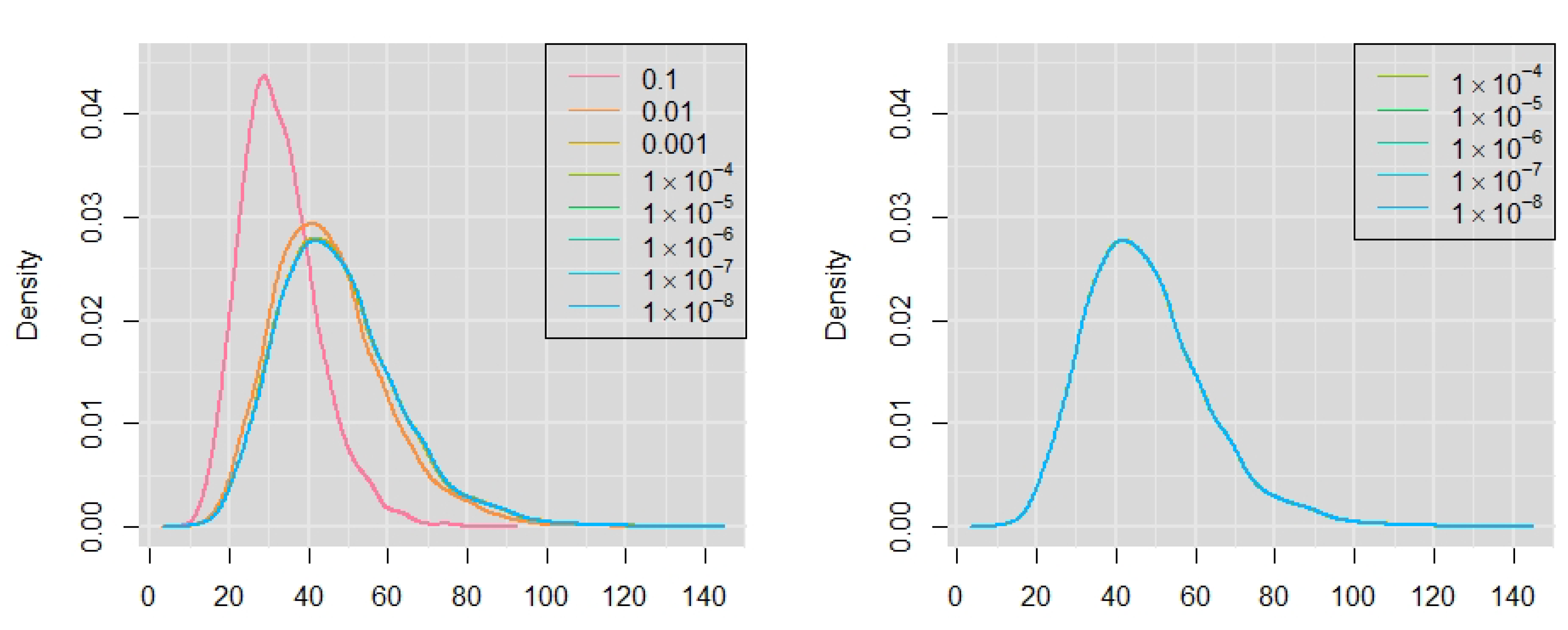
Following these guidelines, for our Bayesian analysis, we will assume noninformative prior distributions with zero mean and large variance for the regression parameters, as well as for the spatial lag parameters included in the proposed models. For the inverse of the dispersion parameters, $\psi =1/\tau$, we will specify Gamma distributions with large variances, so that $\psi \sim G(\alpha ,\alpha )$, with $\alpha$ being a very small value. Estimation will be carried out in OpenBUGS, and also in R-INLA for some specific cases.

Model selection will be performed by using the Deviance Information Criterion (DIC) [37] and the Watanabe-Akaike Information Criterion (WAIC) [38], also known as the widely applicable information criterion, where the models with the lowest values for these criteria would be considered as the best fitting ones. On the one hand, the DIC is based on the posterior distribution of the deviance statistic, a measure of the model’s fit, and it is penalized by the effective number of parameters, which is a measure representing the complexity of the model. On the other hand, the WAIC is based on the logarithm of the pointwise posterior predictive density and receives a penalty specified by a different definition of the effective number of parameters. This criterion has become very popular in the last few years, since it is considered as a fully Bayesian approach (see [23,39]). Given that each of these two measures has its own advantages and drawbacks (see [39]), we will include both of them in our analysis, since we believe the information provided by one can be complemented by the other. Moreover, besides these information criteria values, we will also take into account the predictive accuracy of the fitted models to select the best fitting ones by performing posterior predictive checks on each of the fitted models.

3. Application to the Study of Infant Mortality in Colombia

The data analyzed here have been obtained from the National Statistics Department of Colombia and this specific data set corresponds to 32 departments or geographical units (areas or regions) in this country. For each geographical unit, the available variables are: the number of children under one year of age who died in 2005 (i.e., variable ND), the total number of births in 2005 (i.e., variable NB), an index representing the percentage of the population not having their basic services satisfactorily attended for the same year (i.e., variable NBI), the amount of resources (in thousands of dollars) for academic achievement or education and integral attention for young children provided by the government per household in the year 2005 (i.e., variable Rec), the percentage of women over the age of 18 who had suffered physical violence from their current partners (i.e., variable Viol), the percentage of young people (i.e., between 18 and 24 years) who were able to opt for a higher educational level (i.e., variable HE), and the percentage of children under one year of age who received the third dose of the polio vaccine in the year 2004 (i.e., variable Vac).

A similar version of this data has been previously analyzed by Quintero-Sarmiento, Cepeda-Cuervo and Núñez-Antón [9] and Cepeda-Cuervo, Córdoba and Núñez-Antón [22], where the authors fitted their proposed generalized spatial conditional models to analyze mortality rates for children under five years of age, considering the response variable to be the number of children under five years of age who died in each department in Colombia from 2000 up to 2005. They found evidence of overdispersion and positive spatial autocorrelation in the data set they analyzed, and they were able to capture these specific features in the data set under study with the fitting of the proposed models, where positive significant relations between the variables NBI and the number of deaths for children under five years of age, as well as negative significant relations between the variables Rec and mortality rates. We would like to indicate that the data set here was directly obtained from the National Statistics Department of Colombia because we were unable to have access to the one previously analyzed by other authors and, thus, our analysis is not applied to the same data set.

In this section, we study the mortality rates for children under one year of age in the year 2005, and fit the models previously discussed in Section 2. The explanatory variables that we will include in the study constitute relevant socio-economic indicators that can considerably affect infant mortality (see [22]). In order to specify noninformative prior distributions for the parameters in our Bayesian analysis, we assume independent normal distributions, $N(0,1\times {10}^5)$, for all the regression parameters; that is, ${\beta }_j\sim N(0,1\times {10}^5)$, $j=1,\cdots ,k$, as well as for the spatial association parameter $\rho$. As for the inverse of the dispersion parameters $\tau$, $\psi =1/\tau$, based on the sensitivity analysis performed in Section 3.2 for this specific prior distribution, gamma $G(1\times {10}^{-4},1\times {10}^{-4})$ distributions were assumed. When running the implemented software programs in OpenBUGS, and after 10,000 iterations, a burn in period of 5000 samples and considering a thinning parameter of 10, the MCMC chains showed strong signs of convergence for all of the parameters included in the proposed models.

With the available information in the data set under study, we can approximate infant mortality rates as the number of children under one year of age who died in the year 2005 per 1000 born alive in each of the departments in Colombia. In this way, we can obtain a new variable (i.e., the variable Rates) as:

$${\mathrm{Rates}}_i={\displaystyle \frac{{\mathrm{ND}}_i}{{\mathrm{NB}}_i}}\times 1000,i=1,\cdots ,n$$

(12)

In order to better understand the data under study,

Table 1. Descriptive statistics for the variables available in the study of infant mortality in Colombia.

	Rates	ND	NB	Viol	NBI	Rec	HE	Vac
Mean	25.82	542.88	26,731.59	34.73	37.99	84.29	15.69	69.32
Standard deviation	10.37	444.27	27,567.57	5.64	17.15	64.56	10.52	10.96
Minimum	14.25	16.00	408.00	22.58	9.20	8.02	1.30	42.70
Maximum	49.33	1802.00	115,890.00	44.69	79.20	274.10	52.20	94.70

includes a summary of some descriptive statistics for the available variables in the Colombian mortality rates data set.

Figure 1 shows the spatial distribution of the variable Rates, representing an approximation of infant mortality rates in each department of Colombia for the year 2005. In the map, there are clear indicators of spatial association in the data, as regions with similar values of the variable appear to be grouped together in space. Departments located in the east of the country, belonging to the natural region called the Amazonia, which is located in the Amazonian rain forest, show large values of mortality rates. In addition, for departments located in the central part of the country, surrounding the capital, Bogotá, smaller rates can be observed.

It is important to mention that it has seemed reasonable for authors that have previously analyzed similar data sets to assume that, with regard to infant mortality rates, regions closer in space share somehow similar socio-demographic and economic characteristics, i.e., they can present similar values of infant mortality rates. As observed in the regional map shown in Figure 1, we have reasons to believe that this data set may also exhibit spatial dependence, which must be properly assessed and, if required, it should also be appropriately included in the proposed models to be fitted to this specific data set. An additional issue worth mentioning is the possibility that the aforementioned association may also be related to migration, either to other regions or to the capital. This is a topic that needs to be further explored and the appropriate data sets, if available, where infant mortality rates and migration are related, should be used. However, to our knowledge, such data sets are not available at the moment and, therefore, this issue remains to be further investigated. Moreover, we believe it is out of the scope of the research proposals presented here. Therefore, we will specify a spatial neighborhood structure, represented by the $n\times n$ first order spatial weights matrix $\mathbf{W}=\left[w_{ij}\right]$, standardized by rows, with $w_{ij}=1/n_i$, if i is adjacent, and hence, a neighbor to region j; that is, if they share at least one point in their boundaries, and $w_{ij}=0$, otherwise. Here, $n_i$ is the number of neighbors for the i-th region. The spatial lag of the variable Rates is obtained by multiplying the i-th row of the spatial weights matrix $\mathbf{W}=\left[w_{ij}\right]$, ${\mathbf{W}}_i$, and the $n\times 1$ vector of observations for the variable Rates, that is ${\mathbf{W}}_i\mathbf{Rates}$.

In order to be able to assess the possible existence of spatial dependence in the data, we apply the global Moran’s I contrast [40] to the variable Rates, obtaining a test statistic value of I = 0.3490, providing a p-value = 0.0017. Hence, for the specific data set under study, there is evidence against the null hypothesis that the values of the variable Rates are randomly distributed across the different regions in Colombia. This result can be better seen in a graphical display in Moran’s scatterplot, shown in Figure 2, where the variable Rates is plotted against the spatial lag ${\mathbf{W}}_i\mathbf{Rates}$, and where a red line represents the estimated linear regression line fitted for these two variables. The slope of this regression is precisely Moran’s I statistic and, as can be seen in Figure 2, the values of the variable for each department appear to have a positive significant correlation with the averaged values of the variable in the adjacent regions. Hence, there is substantial evidence for the possible existence of positive spatial autocorrelation in the data that need to be accounted for in the models to be fitted in the following sections for its analysis.

To further confirm the previous conclusions, we have also applied Geary’s C test [41] to the variable Rates, obtaining a value for the C statistic of C = 0.5490, with a p-value = 0.0017. Taking into account that significant values for the C statistic of 1 indicate no spatial autocorrelation for this test, and that values between 0 and 1 indicate positive spatial autocorrelation in the variable under study, the results obtained for our case (i.e., C = 0.5490) suggest further evidence that the variable is not randomly distributed across the regions, but positively correlated.

3.1. Fitting of the Spatial Conditional Overdispersion Models

We assume that the number of children under one year of age who died in 2005 in the ith region; that is, the variable ${\mathrm{ND}}_i$ follows a Poisson distribution with mean ${\mu }_i$. As we are interested in modeling the mortality rates, we will consider that $\mathrm{E}({\mathrm{ND}}_i)={\mu }_i$, with ${\mu }_i={\mathrm{NB}}_i{\lambda }_i$, where ${\mathrm{NB}}_i$ is the total number of births in 2005 (i.e., the variable NB), and ${\lambda }_i$ represents the corresponding mortality rate. Therefore, we include the logarithm of the total number of births $log({\mathrm{NB}}_i)$ in the linear predictor as an offset variable, so that we can write this model as:

$$log\left({\mu }_i\right)=log\left({\mathrm{NB}}_i\right)+{\beta }_0+{\beta }_1{\mathrm{Viol}}_i+{\beta }_2{\mathrm{NBI}}_i+{\beta }_3{\mathrm{Rec}}_i+{\beta }_4{\mathrm{HE}}_i+{\beta }_5{\mathrm{Vac}}_i$$

(13)

Table 2. Parameter estimates, standard deviations and 95% credible intervals in parenthesis for the parameters in the models, and DIC and WAIC values for the different models fitted to the Colombian infant mortality rates data set.

		Poisson	Spatial Conditional Poisson	Negative Binomial	Spatial Conditional Negative Binomial	Normal Poisson	Spatial Conditional Normal Poisson
Intercept	Mean	−4.2960	−4.6131	−4.4647	−5.0672	−4.4330	−4.8410
	SD	(0.0902)	(0.1188)	(0.2109)	(0.2273)	(0.3171)	(0.2900)
	CI	(−4.4710, −4.1210)	(−4.8500, −4.3680)	(−4.9050, −4.1010)	(−5.5530, −4.4670)	(−5.0610, −3.8189)	(−5.4120, −4.3220)
Viol	Mean	0.0066	0.0065	0.0118	0.0112	0.0109	0.0092
	SD	(0.0015)	(0.0015)	(0.0056)	(0.0058)	(0.0060)	(0.0060)
	CI	(0.0036, 0.0096)	(0.0035, 0.0093)	(8.860 × 10${}^{-4}$, 0.0229)	(1.650 × 10${}^{-4}$, 0.0229)	(−9.898 × 10${}^{-4}$, 0.0230)	(−0.0019, 0.0217)
NBI	Mean	0.0155	0.0165	0.0153	0.0167	0.0155	0.0159
	SD	(6.076 × 10${}^{-4}$)	(6.419 × 10${}^{-4}$)	(0.0024)	(0.0023)	(0.0025)	(0.0023)
	CI	(0.0143, 0.0167)	(0.0153, 0.0178)	(0.0104, 0.0200)	(0.0121, 0.0211)	(0.0104, 0.0204)	(0.0113, 0.0203)
Rec	Mean	−4.953 × 10${}^{-4}$	−5.363 × 10${}^{-4}$	−9.818 × 10${}^{-4}$	−7.407 × 10${}^{-4}$	−0.0011	−8.113 × 10${}^{-4}$
	SD	(1.279 × 10${}^{-4}$)	(1.278 × 10${}^{-4}$)	(5.822 × 10${}^{-4}$)	(5.615 × 10${}^{-4}$)	(5.989 × 10${}^{-4}$)	(5.656 × 10${}^{-4}$)
	CI	(−7.454 × 10${}^{-4}$, −2.460 × 10${}^{-4}$)	(−7.881 × 10${}^{-4}$, −2.819 × 10${}^{-4}$)	(−0.0021, 1.756 × 10${}^{-4}$)	(−0.0018, 3.747 × 10${}^{-4}$)	(−0.0023, 1.118 × 10${}^{-4}$)	(−0.0020, 2.760 × 10${}^{-4}$)
HE	Mean	−0.0013	3.117 × 10${}^{-4}$	−0.0058	3.353 × 10${}^{-4}$	−0.0054	−7.355 × 10${}^{-4}$
	SD	(9.218 × 10${}^{-4}$)	(0.0010)	(0.0042)	(0.0045)	(0.0044)	(0.0047)
	CI	(−0.0031, 4.562 × 10${}^{-4}$)	(−0.0017, 0.0023)	(−0.0143, 0.0025)	(−0.0085, 0.0091)	(−0.0140, 0.0033)	(−0.0099, 0.0091)
Vac	Mean	−0.0036	−0.0029	−0.0011	−5.550 × 10${}^{-4}$	−0.0014	−0.0016
	SD	(9.417 × 10${}^{-4}$)	(9.291 × 10${}^{-4}$)	(0.0028)	(0.0028)	(0.0032)	(0.0031)
	CI	(−0.0054, −0.0017)	(−0.0047, −0.0011)	(−0.0065, 0.0045)	(−0.0061, 0.0051)	(−0.0076, 0.0050)	(−0.0083, 0.0043)
$\mathit{\rho }$	Mean	-	0.0095	-	0.0169	-	0.0149
	SD	-	(0.0025)	-	(0.0065)	-	(0.0068)
	CI	-	(0.0045, 0.0144)	-	(0.0041, 0.0295)	-	(6.637 × 10${}^{-4}$, 0.0290)
$\mathit{\tau }$	Mean	-	-	41.5803	46.2603	0.0277	0.0243
	SD	-	-	(13.9969)	(15.4866)	(0.0102)	(0.0088)
	CI	-	-	(20.0300, 73.6512)	(21.9997, 82.7505)	(0.0138, 0.0531)	(0.0121, 0.0460)
		DIC = 491.7	DIC = 480.4	DIC = 362.2	DIC = 360.1	DIC = 308.0	DIC = 307.3
		WAIC = 524.0	WAIC = 519.6	WAIC = 361.8	WAIC = 360.3	WAIC = 302.3	WAIC = 301.3

includes the corresponding parameter estimates for the fitting of the Poisson model with regression structure given in Equation (13), together with its standard deviations and 95% credible intervals in parenthesis, when fitted to the Colombia infant mortality rates data set. For this model, the resulting information criteria values where DIC = 491.7 and WAIC = 524.0. Based on the estimations for the regression coefficients for this model, we can observe that all the explanatory variables, except HE, are statistically significant, as none of their 95% credible intervals includes the value zero. However, these reported results should not be taken as an indication of a good model’s fit, mainly because it could be a consequence of fitting the model without taking into account the existence of overdispersion. In fact, if we plot the estimated mean and variance obtained by the fitting of this model (see Figure 3), where the blue line represents that its mean equals its variance, we notice that most of the estimated variance values from the Poisson model are larger than the mean, which may be a clear indication that the assumption of equidispersion of the Poisson distribution does not seem to hold for this data set.

Therefore and based on the possible existence of overdispersion, we have fitted the overdispersion models mentioned in the previous section, starting with the normal Poisson model with regression structure given by Equation (14), and the negative binomial model with regression structure as in the Poisson model in Equation (13). These models show considerable improvements in their DIC and WAIC values when compared to those for the Poisson model. That is, resulting values were DIC = 308.0 and WAIC = 302.3 for the normal Poisson model, and DIC = 362.2 and WAIC = 361.8 for the negative binomial model. Moreover, if we carefully observe the results for the 95% credible intervals for the estimated coefficients after fitting the normal Poisson model, we notice that, except for NBI, all the other variables are statistically nonsignificant. In the case of the fitting of the negative binomial model, only the variables NBI and Viol are statistically significant. These results are justified because these models have taken into account the overdispersion in the data set under study and, therefore, these credible intervals become wider than those obtained when fitting the Poisson model.

$$log({\mu }_i)=log\left({\mathrm{NB}}_i\right)+{\beta }_0+{\beta }_1{\mathrm{Viol}}_i+{\beta }_2{\mathrm{NBI}}_i+{\beta }_3{\mathrm{Rec}}_i+{\beta }_4{\mathrm{HE}}_i+{\beta }_5{\mathrm{Vac}}_i+{\nu }_i,{\nu }_i\sim N(0,\tau )$$

(14)

In addition, to be able to account for the possible spatial dependence present in the data set under study, we have also fitted the spatial conditional Poisson and negative binomial models, with regression structures given by Equation (15), where the spatial lag of the variable Rates is also included in these models. That is, we have that:

$$log({\mu }_i)=log\left({\mathrm{NB}}_i\right)+{\beta }_0+{\beta }_1{\mathrm{Viol}}_i+{\beta }_2{\mathrm{NBI}}_i+{\beta }_3{\mathrm{Rec}}_i+{\beta }_4{\mathrm{HE}}_i+{\beta }_5{\mathrm{Vac}}_i+\rho {\mathbf{W}}_i\mathbf{Rates}$$

(15)

Finally, we have also fitted the spatial conditional normal Poisson model with regression structure given in Equation (16), with reported information criteria values of DIC = 307.3 and WAIC = 301.3, these being the lowest information criteria values obtained so far when compared to the rest of the models. In addition, the estimated value for the spatial lag parameter, $\rho$, was $\widehat{\rho }=0.0149\left(0.0068\right)$, with the value zero not included in its 95% credible interval, a clear evidence for the existence of positive spatial autocorrelation in the data. Moreover, the estimated dispersion parameter was $\widehat{\tau }=0.0243\left(0.0088\right)$, also indicating that, besides explaining the spatial dependence, this model also captures the overdispersion, allowing for an extra variation given that a specific random effect has been included for this purpose in this model.

$$\begin{array}{cc}\hfill log({\mu }_i)=& log\left({\mathrm{NB}}_i\right)+{\beta }_0+{\beta }_1{\mathrm{Viol}}_i+{\beta }_2{\mathrm{NBI}}_i+{\beta }_3{\mathrm{Rec}}_i+{\beta }_4{\mathrm{HE}}_i+{\beta }_5{\mathrm{Vac}}_i+\rho {\mathbf{W}}_i\mathbf{Rates}+{\nu }_i,\hfill \\ \hfill & {\nu }_i\sim N(0,\tau )\hfill \end{array}$$

(16)

From the results reported in Table 2, the lowest DIC and WAIC values were obtained for the spatial conditional normal Poisson model, which was considered therefore the best fitting model. A variable selection process was performed afterwards for this model by fitting reduced versions and comparing the information criteria values obtained for the different models. The results for some of the fitted models shown in

Table 3. Parameter estimates, standard deviations and 95% credible intervals in parenthesis for the parameters in the models, and Deviance Information Criterion (DIC) and Watanabe-Akaike Information Criterion (WAIC) values for some of the reduced versions of the spatial conditional normal Poisson model fitted to the Colombian infant mortality rates data set.

		Intercept	Viol	NBI	Rec	Vac	$\mathit{\rho }$	$\mathit{\tau }$
DIC = 307.3	Mean	−4.8298	0.0087	0.0165	−9.389 × 10${}^{-4}$	−0.0017	0.0145	0.0230
WAIC = 301.7	SD	(0.3218)	(0.0055)	(0.0018)	(5.362 × 10${}^{-4}$)	(0.0029)	(0.0061)	(0.0084)
	CI	(−5.4881, −4.2110)	(−0.0019, 0.0197)	(0.0127, 0.0201)	(−0.0020, 1.010 × 10${}^{-4}$)	(−0.0072, 0.0042)	(0.0022, 0.0264)	(0.0111, 0.0442)
DIC = 307.8	Mean	−4.5858	-	0.0165	−0.0011	−8.340 × 10${}^{-4}$	0.0153	0.0247
WAIC = 302.4	SD	(0.2861)	-	(0.0019)	(5.353 × 10${}^{-4}$)	(0.0030)	(0.0063)	(0.0086)
	CI	(−5.1450, −4.0230)	-	(0.0127, 0.0204)	(−0.0022, −9.296 × 10${}^{-5}$)	(−0.0069, 0.0051)	(0.0028, 0.0277)	(0.0125, 0.0450)
DIC = 307.5	Mean	−5.1301	0.0116	0.0158	-	−9.405 × 10${}^{-4}$	0.0183	0.0250
WAIC = 301.8	SD	(0.2881)	(0.0054)	(0.0019)	-	(0.0030)	(0.0059)	(0.0085)
	CI	(−5.6960, −4.5760)	(0.0011, 0.0223)	(0.0121, 0.0196)	-	(−0.0068, 0.0050)	(0.0068, 0.0301)	(0.0125, 0.0457)
DIC = 306.8	Mean	−4.9505	0.0083	0.0165	−8.274 × 10${}^{-4}$	-	0.0150	0.0225
WAIC = 301.2	SD	(0.2588)	(0.0055)	(0.0018)	(5.446 × 10${}^{-4}$)	-	(0.0060)	(0.0080)
	CI	(−5.4700, −4.4500)	(−0.0026, 0.0194)	(0.0128, 0.0200)	(−0.0019, 2.409 × 10${}^{-4}$)	-	(0.0030, 0.0270)	(0.0113, 0.0421)
DIC = 307.8	Mean	−4.8702	-	0.0157	-	3.069 × 10${}^{-4}$	0.0207	0.0285
WAIC = 302.0	SD	(0.2594)	-	(0.0020)	-	(0.0031)	(0.0061)	(0.0095)
	CI	(−5.3800, −4.3700)	-	(0.0118, 0.0197)	-	(−0.0057, 0.0064)	(0.0090, 0.0324)	(0.0147, 0.0505)
DIC = 307.4	Mean	−4.6479	-	0.0167	−0.0011	-	0.0151	0.0233
WAIC = 302.3	SD	(0.1660)	-	(0.0018)	(4.982 × 10${}^{-4}$)	-	(0.0061)	(0.0080)
	CI	(−4.9660, −4.3240)	-	(0.0132, 0.0202)	(−0.0021, −1.824 × 10${}^{-4}$)	-	(0.0033, 0.0272)	(0.0119, 0.0430)
DIC = 306.9	Mean	−5.1912	0.0114	0.0159	-	-	0.0184	0.0241
WAIC = 301.4	SD	(0.2136)	(0.0053)	(0.0018)	-	-	(0.0059)	(0.0082)
	CI	(−5.6120, −4.7650)	(0.0010, 0.0221)	(0.0124, 0.0193)	-	-	(0.0067, 0.0298)	(0.0123, 0.0437)
DIC = 308.2	Mean	−4.8478	-	0.0156	-	-	0.0208	0.0272
WAIC = 303.4	SD	(0.1439)	-	(0.0019)	-	-	(0.0059)	(0.0091)
	CI	(−5.1390, −4.5740)	-	(0.0119, 0.0194)	-	-	(0.0094, 0.0323)	(0.0143, 0.0490)

indicate that the model with the lowest information criteria values, i.e., DIC = 306.8 and WAIC = 301.2, is the one which includes the variables Viol, NBI and Rec, but in this model, the variables Viol and Rec are not statistically significant, since zero is contained in the 95% credible interval for the estimated coefficients for each of these variables.

The model including the variables NBI and Rec with regression structure given by Equation (17), which provided information criteria values of DIC = 307.4 and WAIC = 302.3, could be a good candidate for fitting the data under study. In this model, according to its 95% credible intervals, all of the estimated coefficients are statistically significant. The estimated coefficient for the variable NBI was $\widehat{{\beta }_1}=0.0167\left(0.0018\right)$, which indicates that, according to the model fitted to this data, infant mortality rates have a statistically significant positive association with the percentage of people with unsatisfied basic needs. With regard to the estimated coefficient for the variable Rec, it was $\widehat{{\beta }_2}=-0.0011$(4.982 × 10${}^{-4}$), a fact that could be an indication of a statistically significant negative association between infant mortality rates and the amount of resources provided for academic achievement. In addition, the estimated coefficient for the spatial term has a positive value of $\hat{\rho }=0.0151\left(0.0061\right)$, again a clear evidence of the presence of positive spatial autocorrelation in the data.

$$log({\mu }_i)=log\left({\mathrm{NB}}_i\right)+{\beta }_0+{\beta }_1{\mathrm{NBI}}_i+{\beta }_2{\mathrm{Rec}}_i+\rho {\mathbf{W}}_i\mathbf{Rates}+{\nu }_i,{\nu }_i\sim N(0,\tau )$$

(17)

It is worth mentioning that the model providing information criteria values of DIC = 306.9 and WAIC = 301.4, which correspond to the model containing the variables NBI and Viol, with a regression structure given by Equation (18), should also be considered as a good candidate for fitting the data set under study, where, based on their 95% credible intervals, all of the estimated coefficients are statistically significant. The estimated coefficient for the variable NBI has a value of $\widehat{{\beta }_2}=0.0159\left(0.0018\right)$, a very similar value to that obtained in the previous model for this specific coefficient. In addition, the estimated coefficient for the variable Viol was $\widehat{{\beta }_1}=0.0114\left(0.0053\right)$, implying that infant mortality rates may have a statistically significant positive relation with the percent of women who suffered any type of physical abuse from their current partner. The spatial coefficient estimated value was $\hat{\rho }=0.0184\left(0.0059\right)$, which represents further evidence of the presence of positive spatial autocorrelation in the data.

$$log({\mu }_i)=log\left({\mathrm{NB}}_i\right)+{\beta }_0+{\beta }_1{\mathrm{Viol}}_i+{\beta }_2{\mathrm{NBI}}_i+\rho {\mathbf{W}}_i\mathbf{Rates}+{\nu }_i,{\nu }_i\sim N(0,\tau )$$

(18)

In order to provide some information that could be useful for the readers about the size of the effects of the explanatory variables in the models, we have computed estimations of the marginal effects at the means for these variables in the spatial conditional normal Poisson models in Equations (17) and (18), which are reported in

Table 4. Marginal effects at the means for the spatial conditional normal Poisson models in Equations (17) and (18) fitted to the Colombian infant mortality rates data set.

		Mean	SD	95% CI
Model in Equation (17)	NBI	3.9981 × 10${}^{-4}$	(4.3043 × 10${}^{-5}$)	(3.1469 × 10${}^{-4}$, 4.8580 × 10${}^{-4}$)
	Rec	−2.6978 × 10${}^{-5}$	(1.2012 × 10${}^{-5}$)	(−5.0980 × 10${}^{-5}$, −4.2588 × 10${}^{-6}$)
Model in Equation (18)	Viol	2.7189 × 10${}^{-4}$	(1.2728 × 10${}^{-4}$)	(2.4744 × 10${}^{-5}$, 5.2951 × 10${}^{-4}$)
	NBI	3.7891 × 10${}^{-4}$	(4.2576 × 10${}^{-5}$)	(2.9550 × 10${}^{-4}$, 4.6250 × 10${}^{-4}$)

. For the variable NBI in the model in Equation (17), this estimated marginal effect was 3.9981 × 10${}^{-4}$, which means that with an increment of 1 percentage point in the variable NBI, the mortality rate would be increased by a 0.039981%, when the other variables are set at their mean value. Although this represents a very small effect on the infant mortality rate, according to the credible interval (3.1469 × 10${}^{-4}$, 4.8580 × 10${}^{-4}$), it is indeed significant. Moreover, small effects, but significant according to their credible intervals, were also obtained for the variable Rec in this model and for the variables Viol and NBI for the model in Equation (18).

In order to assess the convergence of the MCMC chains for the fitted models, we have computed the effective sample size for estimating the means, (i.e., ${\mathrm{N}}_{\mathrm{eff}}$), and the potential scale reduction factor (i.e., $\hat{\mathrm{R}}$) for each parameter’s MCMC chain. For brevity of exposition, the obtained results are reported in

Table 5. Convergence diagnostics for the spatial conditional normal Poisson models in Equations (17) and (18) fitted to the Colombian infant mortality rates data set.

		Intercept	Viol	NBI	Rec	$\mathit{\rho }$	$\mathit{\tau }$
Model in Equation (17)	${\mathrm{N}}_{\mathrm{eff}}$	13,000	-	15,000	11,000	7300	1500
	$\widehat{\mathrm{R}}$	1.0011	-	1.0010	1.0011	1.0012	1.0023
Model in Equation (18)	${\mathrm{N}}_{\mathrm{eff}}$	2700	9600	3400	-	7800	13,000
	$\widehat{\mathrm{R}}$	1.0016	1.0011	1.0015	-	1.0012	1.0011

only for the models in Equations (17) and (18).

The values ${\mathrm{N}}_{\mathrm{eff}}$ represent the equivalent number of independent samples in each parameter’s MCMC chain. It is often considered that a minimum of 100 independent simulations is a sufficient number for performing reasonable posterior inference (see [23]). Therefore, a desirable value for ${\mathrm{N}}_{\mathrm{eff}}$ would be any number of at least 100. We have simulated 3 Markov chains, with 10,000 iterations and discarded the first 5000 samples from each one, which leaves us with a total of 15,000 samples. Taking this into account and considering that the values of ${\mathrm{N}}_{\mathrm{eff}}$ for the chains of all the estimated parameters obtained from the fitting of models in Equations (17) and (18), reported in Table 5, are larger than 1000, we can conclude that we have enough simulations to correctly approximate the target distribution and that the correlation in the chains should not affect posterior inference on the parameters. Moreover, the values $\hat{\mathrm{R}}$ are an estimation of the potential scale reduction factor (see [42]). Values closer to 1 indicate convergence of the chain, whereas when values larger than 1.1 are obtained, it is considered that further simulations need to be computed in order to improve posterior inference. In this specific application, all of the $\hat{\mathrm{R}}$ values are approximately one, which suggests that the chains for all of the parameters have successfully converged to the target distribution.

As a summary of this section, we believe it may be convenient to mention that the results obtained from the fitting of these models in Equations (17) and (18) are consistent with the previous results obtained in Cepeda-Cuervo, Córdoba and Núñez-Antón [22] for a similar data set. This fact is an illustration of the usefulness of the spatial conditional overdispersion models for being able to explain spatial dependence and overdispersion in applications for real data sets.

3.2. Sensitivity Analysis for the Variance of the Prior Distributions

The prior distribution $G(\alpha ,\alpha )$, assumed for the inverse of the variance parameter $\tau$ for the random effects, that is, for the precision parameter $\psi =1/\tau$, can have a significant effect on the inferential process, so inference may be quite sensitive to the choice of the fixed parameters $\alpha$ in this gamma distribution (see [36]). Therefore, in order to better assess this effect and select prior distributions where it is limited or at least controlled for, we have performed a sensitivity analysis for the best fitting model in the previous section, the spatial conditional normal Poisson model with regression structure given by Equation (17), considering different possible values for $\alpha$ in the gamma prior distribution $\psi \sim G(\alpha ,\alpha )$ for the precision parameter in the random effects, from $\alpha =0.1$ to $\alpha =1\times {10}^{-8}$. Results are included in

Table 6. Posterior means for parameter estimates together with standard deviations, DIC and WAIC values, for the spatial conditional normal Poisson model in the analysis of the Colombian infant mortality rates data set with different prior distributions for the precision parameter of the random effects.

	Intercept	NBI	Rec	$\mathit{\rho }$	$\mathit{\tau }$	DIC	WAIC
$\alpha =0.1$	−4.6488	0.0167	−0.0012	0.0153	0.0332	306.5	298.2
	(0.1956)	(0.0022)	(6.020 × 10${}^{-4}$)	(0.0073)	(0.0104)
$\alpha =0.01$	−4.6455	0.0167	−0.0011	0.0151	0.0245	307.2	301.6
	(0.1727)	(0.0018)	(5.154 × 10${}^{-4}$)	(0.0064)	(0.0083)
$\alpha =0.001$	−4.6469	0.0167	−0.0011	0.0151	0.0234	307.4	302.3
	(0.1680)	(0.0018)	(5.017 × 10${}^{-4}$)	(0.0062)	(0.0080)
$\alpha =1\times {10}^{-4}$	−4.6479	0.0167	−0.0011	0.0151	0.0233	307.4	302.3
	(0.1660)	(0.0018)	(4.982 × 10${}^{-4}$)	(0.0061)	(0.0080)
$\alpha =1\times {10}^{-5}$	−4.6480	0.0167	−0.0011	0.0151	0.0233	307.4	302.3
	(0.1661)	(0.0018)	(4.981 × 10${}^{-4}$)	(0.0061)	(0.0080)
$\alpha =1\times {10}^{-6}$	−4.6480	0.0167	−0.0011	0.0151	0.0233	307.4	302.3
	(0.1660)	(0.0018)	(4.981 × 10${}^{-4}$)	(0.0061)	(0.0080)
$\alpha =1\times {10}^{-7}$	−4.6480	0.0167	−0.0011	0.0151	0.0233	307.4	302.3
	(0.1660)	(0.0018)	(4.981 × 10${}^{-4}$)	(0.0061)	(0.0080)
$\alpha =1\times {10}^{-8}$	−4.6480	0.0167	−0.0011	0.0151	0.0233	307.4	302.3
	(0.1660)	(0.0018)	(4.981 × 10${}^{-4}$)	(0.0061)	(0.0080)

, where we can observe that for values of $\alpha =1\times {10}^{-4}$, as well as for smaller values, there were only small differences in the estimates in the third decimal place for a few cases. If we also look at the posterior marginal densities for the estimated precision parameter $\psi$ (see right panel in Figure 4), no changes are observed when setting the values for $\alpha$ in the prior distributions for the last five values considered here (i.e., from $\alpha =1\times {10}^{-4}$ up to $\alpha =1\times {10}^{-8}$). Therefore, we believe the choice of the value $\alpha =1\times {10}^{-4}$ is well justified and, in addition, it does not appear to represent any undesirable influence on the inferential process considered here.

3.3. Fitting of the Generalized Spatial Conditional Normal Poisson Model

For all of the aforementioned fitted models, it is assumed that the dispersion parameter (i.e., $\tau$) is constant, a fact that could not always be a reasonable assumption. Hence, we will allow the dispersion parameter to vary with some explanatory variables by considering the so-called generalized spatial conditional models (see [22]). After fitting the generalized spatial conditional normal Poisson model for the infant mortality data in Colombia and, performing a variable selection process, we have concluded that the best fitting model was the one where the mean model contains the spatial lag and the dispersion model includes the variable NBI, so that:

$$\begin{array}{ccc}\hfill log({\mu }_i)& =& log\left({\mathrm{NB}}_i\right)+\beta +\rho {\mathbf{W}}_i\mathbf{Rates}+{\nu }_i,{\nu }_i\sim N(0,{\tau }_i)\hfill \\ \hfill log\left({\tau }_i\right)& =& {\gamma }_0+{\gamma }_1{\mathrm{NBI}}_i\hfill \end{array}$$

(19)

Table 7. Parameter estimates, standard deviations and 95% credible intervals for the estimated means in parenthesis, DIC and WAIC values, for the generalized spatial conditional normal Poisson model fitted to the Colombian infant mortality rates data set.

		$\mathit{\mu }$ Intercept: $\mathit{\beta }$	$\mathit{\rho }$	$\mathit{\tau }$ Intercept: ${\mathit{\gamma }}_0$	NBI
DIC = 308.0	Mean	−4.9262	0.0431	−4.2186	0.0430
WAIC = 299.1	SD	(0.2275)	(0.0093)	(0.6165)	(0.0145)
	CI	(−5.3620, −4.4780)	(0.0249, 0.0608)	(−5.4200, −2.9998)	(0.0161, 0.0727)

reports the results from the fitting of the model in Equation (19). The DIC = 308.0 and WAIC = 299.1 values from the fitting of this model are quite similar to those obtained when fitting the spatial conditional normal Poisson model and, therefore, this does not result in a significant improvement in the model’s fitting. However, we believe that there are some very interesting features that can be noticed from these two fittings. On the one hand, the mean of the estimated coefficient for the variable NBI in the dispersion model was $\widehat{{\gamma }_1}=0.0430\left(0.0145\right)$ and, according to its 95% credible interval, this variable is statistically significant, which could indicate that the dispersion varies according to the variable NBI in such a way that in regions where the percentage of the population not having basic services satisfactorily attended is larger, the dispersion increases. On the other hand, the spatial parameter estimate in the mean model has a mean with a positive value of $\hat{\rho }=0.0431\left(0.0093\right)$ and, in addition, according to its 95% credible interval, it is also statistically significant. The significance of $\rho$ constitutes a clear evidence for the presence of positive spatial autocorrelation, which is appropriately captured by the fitting of this model. Taking these facts into consideration, the fitting of these generalized spatial conditional models would be well justified. In addition to being able to model the spatial dependence in the data, it also explains their nonconstant dispersion.

As part of the posterior predictive checks required to better assess the fit of a model, Figure 5 includes the scatterplots for the observed mortality rates versus the predicted mortality rates for some of the fitted models. From the plots in Figure 5a,b, we can mention that the spatial conditional normal Poisson models in Equations (17) and (18) show high accuracy in the prediction of mortality rates for observed rates under 40 whereas, for some of the values larger than 40, predictions slightly deviate from the observed values. The scatterplot included in Figure 5c for the generalized spatial conditional normal Poisson model in Equation (19) shows a considerable improvement, mainly because values of the mortality rates larger than 40 are now more accurately predicted.

Figure 6 includes histograms of the posterior predictive distributions for the means over replicated simulations of the mortality rates, estimated from the fitting of the spatial conditional normal Poisson model in Equation (17) (see Figure 6a) and Equation (18) (see Figure 6b), and by the generalized spatial conditional normal Poisson model in Equation (19) (see Figure 6c). As we can see from these figures, they show how the means of the replicated data vary with respect to the actual mean of the observed values, a fact suggesting that the considered models offer an adequate fit to the data set under study.

3.4. Comparisons to the BYM Model

In order to be able to compare the performance between the previous models and the BYM model, we have decided to select the best fitting model we have so far, which is the spatial conditional normal Poisson model, and compare its fitting to that of the BYM model. In order to do so, we have fitted the BYM model with regression structure given by:

$$log({\mu }_i)=log\left({\mathrm{NB}}_i\right)+{\beta }_0+{\beta }_1{\mathrm{Viol}}_i+{\beta }_2{\mathrm{NBI}}_i+{\beta }_3{\mathrm{Rec}}_i+{\beta }_4{\mathrm{Vac}}_i+{\nu }_i+{\eta }_i,$$

(20)

where ${\nu }_i,i=1,\cdots ,n$ is a set of normally distributed random effects with $\mathrm{Var}\left({\nu }_i\right)=\tau$, with $\tau >0$, and ${\eta }_i,i=1,\cdots ,n$ is a set of spatially structured random effects following an intrinsic CAR prior distribution, with variance parameter ${\tau }_{\eta }$. As in the previous models, we assume noninformative normal priors for the regression parameters; that is, $N(0,1\times {10}^{-5})$ and, for the precision parameters $\psi =1/\tau$ and ${\psi }_{\eta }=1/{\tau }_{\eta }$, we also assume noninformative prior gamma $G(1\times {10}^{-4},1\times {10}^{-4})$ distributions. Finally, for the BYM model, we assume the same first order neighborhood structure as before.

The fitting of this model in OpenBUGS is very unstable, since it showed drastic changes if we slightly changed the assumed values for the prior distributions, especially in the estimated values for the variance parameter ${\tau }_{\eta }$ of the spatially structured random effects. In addition, in most cases, the effective number of parameters resulted in negative values, which could be a clear sign of conflict between the prior distribution and the data (see [37]). For the reasons we have just described here, and in order to be able to compare the performance of both models when fitting them to the data set under study, we have fitted both the spatial conditional normal Poisson model in Equation (21) and the BYM model in Equation (20) in R-INLA, by setting the same values for the prior distributions, so that more stable results were provided. Moreover, we have also fitted reduced versions of these models.

$$log({\mu }_i)=log\left({\mathrm{NB}}_i\right)+{\beta }_0+{\beta }_1{\mathrm{Viol}}_i+{\beta }_2{\mathrm{NBI}}_i+{\beta }_3{\mathrm{Rec}}_i+{\beta }_4{\mathrm{Vac}}_i+\rho {\mathbf{W}}_i\mathbf{Rates}+{\nu }_i,$$

(21)

where ${\nu }_i,i=1,\cdots ,n$ is a set of normally distributed random effects with $\mathrm{Var}\left({\nu }_i\right)=\tau$. Results for the estimation of the spatial conditional normal Poisson model in Equation (21) are reported in

Table 8. Parameter estimates, standard deviations and 95% credible intervals for the estimated means in parenthesis, DIC and WAIC values for the reduced versions of the spatial conditional normal Poisson model fitted in INLA to the Colombian infant mortality rates data set.

		Intercept	Viol	NBI	Rec	Vac	$\mathit{\rho }$	$\mathit{\tau }$
DIC = 307.3	Mean	−4.8473	0.0087	0.0164	−8.938 × 10${}^{-4}$	−0.0015	0.0148	0.0231
WAIC = 301.9	SD	(0.3241)	(0.0057)	(0.0018)	(5.425 × 10${}^{-4}$)	(0.0029)	(0.0061)	(0.0082)
	CI	(−5.4930, −4.2117)	(−0.0024, 0.0200)	(0.0127, 0.0200)	(−0.0020, 1.775 × 10${}^{-4}$)	(−0.0073, 0.0043)	(0.0028, 0.0269)	(0.0114, 0.0433)
DIC = 307.7	Mean	−4.5846	-	0.0165	−0.0011	−8.525 × 10${}^{-4}$	0.0153	0.0243
WAIC = 302.3	SD	(0.2806)	-	(0.0019)	(5.295 × 10${}^{-4}$)	(0.0030)	(0.0062)	(0.0084)
	CI	(−5.1419, −4.0332)	-	(0.0128, 0.0202)	(−0.0022, −1.062 × 10${}^{-4}$)	(−0.0067, 0.0051)	(0.0031, 0.0276)	(0.0123, 0.0450)
DIC = 307.4	Mean	−5.1410	0.0116	0.0158	-	−8.776 × 10${}^{-4}$	0.0185	0.0250
WAIC = 301.9	SD	(0.2810)	(0.0056)	(0.0019)	-	(0.0030)	(0.0058)	(0.0086)
	CI	(−5.7002, −4.5905)	(6.159 × 10${}^{-4}$, 0.0227)	(0.0121, 0.0195)	-	(−0.0068, 0.0051)	(0.0070, 0.0301)	(0.0127, 0.0461)
DIC = 306.9	Mean	−4.9464	0.0083	0.0166	−8.587 × 10${}^{-4}$	-	0.0149	0.0224
WAIC = 301.5	SD	(0.2573)	(0.0055)	(0.0018)	(5.312 × 10${}^{-4}$)	-	(0.0060)	(0.0078)
	CI	(−5.4577, −4.4400)	(−0.0026, 0.0193)	(0.0130, 0.0201)	(−0.0019, 1.898 × 10${}^{-4}$)	-	(0.0030, 0.0267)	(0.0113, 0.0416)
DIC = 307.9	Mean	−4.8797	-	0.0158	-	3.763 × 10${}^{-4}$	0.0208	0.0285
WAIC = 302.3	SD	(0.2624)	-	(0.0020)	-	(0.0031)	(0.0060)	(0.0095)
	CI	(−5.4002, −4.3646)	-	(0.0118, 0.0197)	-	(−0.0058, 0.0066)	(0.0089, 0.0328)	(0.0148, 0.0516)
DIC = 307.3	Mean	−4.6489	-	0.0166	−0.0011	-	0.0153	0.0234
WAIC = 302.0	SD	(0.1671)	-	(0.0018)	(5.120 × 10${}^{-4}$)	-	(0.0061)	(0.0080)
	CI	(−4.9791, −4.3188)	-	(0.0130, 0.0202)	(−0.0021, −1.139 × 10${}^{-4}$)	-	(0.0033, 0.0274)	(0.0120, 0.0429)
DIC = 307.1	Mean	−5.1920	0.0113	0.0160	-	-	0.0184	0.0241
WAIC = 301.6	SD	(0.2149)	(0.0054)	(0.0018)	-	-	(0.0058)	(0.0081)
	CI	(−5.6190, −4.7698)	(6.868 × 10${}^{-4}$, 0.0220)	(0.0124, 0.0195)	-	-	(0.0071, 0.0298)	(0.0124, 0.0439)
DIC = 307.6	Mean	−4.8535	-	0.0157	-	-	0.0209	0.0272
WAIC = 302.3	SD	(0.1475)	-	(0.0019)	-	-	(0.0059)	(0.0089)
	CI	(−5.1451, −4.5630)	-	(0.0120, 0.0195)	-	-	(0.0093, 0.0326)	(0.0143, 0.0490)

, and those for the BYM model in Equation (20) are included in

Table 9. Parameter estimates, standard deviations and 95% credible intervals for the estimated means in parenthesis, DIC and WAIC values for the reduced versions of the BYM model fitted in INLA to the Colombian infant mortality rates data set.

		Intercept	Viol	NBI	Rec	Vac	$\mathit{\tau }$	${\mathit{\tau }}_{\mathit{\eta }}$
DIC = 307.9	Mean	−4.4748	0.0067	0.0173	−0.0010	−9.456 × 10${}^{-4}$	0.0224	0.0260
WAIC = 302.7	SD	(0.3265)	(0.0073)	(0.0021)	(6.144 × 10${}^{-4}$)	(0.0031)	(0.0141)	(0.0251)
	CI	(−5.1240, −3.8324)	(−0.0082, 0.0207)	(0.0132, 0.0213)	(−0.0022, 1.819 × 10${}^{-4}$)	(−0.0070, 0.0051)	(0.0073, 0.0601)	(0.0014, 0.0910)
DIC = 308.0	Mean	−4.2825	-	0.0174	−0.0010	−4.280 × 10${}^{-4}$	0.0185	0.0356
WAIC = 303.2	SD	(0.2439)	-	(0.0020)	(6.309 × 10${}^{-4}$)	(0.0030)	(0.0123)	(0.0305)
	CI	(−4.7664, −3.8020)	-	(0.0133, 0.0214)	(−0.0023, 2.147 × 10${}^{-4}$)	(−0.0062, 0.0055)	(0.0052, 0.0514)	(0.0044, 0.1147)
DIC = 307.9	Mean	−4.5923	0.0058	0.0169	-	1.905 × 10${}^{-4}$	0.0128	0.0668
WAIC = 302.8	SD	(0.3326)	(0.0082)	(0.0022)	-	(0.0030)	(0.0095)	(0.0477)
	CI	(−5.2487, −3.9345)	(−0.0106, 0.0216)	(0.0125, 0.0211)	-	(−0.0056, 0.0060)	(0.0024, 0.0377)	(0.0166, 0.1946)
DIC = 307.5	Mean	−4.5267	0.0061	0.0174	−9.647 × 10${}^{-4}$	-	0.0199	0.0302
WAIC = 302.3	SD	(0.2620)	(0.0071)	(0.0020)	(5.953 × 10${}^{-4}$)	-	(0.0129)	(0.0267)
	CI	(−5.0379, −4.0010)	(−0.0084, 0.0199)	(0.0133, 0.0213)	(−0.0021, 1.967 × 10${}^{-4}$)	-	(0.0061, 0.0544)	(0.0028, 0.0991)
DIC = 307.9	Mean	−4.4211	-	0.0171	-	5.190 × 10${}^{-4}$	0.0097	0.0742
WAIC = 303.1	SD	(0.2248)	-	(0.0021)	-	(0.0028)	(0.0076)	(0.0503)
	CI	(−4.8694, −3.9808)	-	(0.0129, 0.0212)	-	(−0.0050, 0.0062)	(0.0014, 0.0295)	(0.0214, 0.2088)
DIC = 307.6	Mean	−4.3162	-	0.0174	−9.695 × 10${}^{-4}$	-	0.0170	0.0367
WAIC = 302.9	SD	(0.0889)	-	(0.0020)	(6.078 × 10${}^{-4}$)	-	(0.0113)	(0.0301)
	CI	(−4.4904, −4.1392)	-	(0.0135, 0.0213)	(−0.0022, 2.002 × 10${}^{-4}$)	-	(0.0047, 0.0470)	(0.0055, 0.1151)
DIC = 307.6	Mean	−4.5740	0.0057	0.0168	-	-	0.0114	0.0668
WAIC = 302.7	SD	(0.2781)	(0.0079)	(0.0021)	-	-	(0.0085)	(0.0467)
	CI	(−5.1153, −4.0184)	(−0.0102, 0.0211)	(0.0126, 0.0209)	-	-	(0.0020, 0.0337)	(0.0175, 0.1914)
DIC = 307.6	Mean	−4.3831	-	0.0170	-	-	0.0091	0.0718
WAIC = 303.8	SD	(0.0794)	-	(0.0020)	-	-	(0.0071)	(0.0475)
	CI	(−4.5384, −4.2244)	-	(0.0129, 0.0210)	-	-	(0.0013, 0.0275)	(0.0212, 0.1992)

, as well as estimations of reduced versions of these models.

If we compare the results from the fitting of the spatial conditional normal Poisson model in OpenBUGS in Table 3 with the one in INLA in Table 8, we can see that reported results are quite similar. In some cases, the means of the estimated parameters only differ in the third decimal place and, only for very few cases, in the second decimal place. This also occurs for the estimations of the variance parameter for the random effects, where we can only observe differences in the third decimal place for some cases. Even though the estimations are very similar, it must be emphasized that the computation time that R-INLA used for the fitting of each one of the models reported in Table 8 was much smaller than the one used by OpenBUGS for the same model. With regard to the information criteria values for the fitted models (i.e., the DIC and WAIC values) reported in Table 9 for the BYM model, as well as those reported in Table 8 for the spatial conditional normal Poisson model, we can see that the WAIC values indicate a moderately better fit for the spatial conditional normal Poisson model whereas differences in the DIC values are minimal and do not favor any of these models in particular. Comparison between the performance of the spatial conditional normal Poisson and the BYM fitted models can be better explored in Figure 7, where scatterplots of the observed versus the estimated values obtained from the fitting of some of the reduced versions of these models are shown. In addition, there are certain points about the fitting of the BYM model that are worth being mentioned.

For the BYM models reported in Table 9, the estimated variance parameters for both the spatially correlated and the uncorrelated random effects show overall quite large standard deviations. For instance, in the case of the model with regression structure given by Equation (20), the estimated variance parameters for the random effects were $\widehat{{\tau }_{\eta }}=0.0260\left(0.0251\right)$ and $\hat{\tau }=0.0224\left(0.0141\right)$, making it difficult to interpret them, especially to explain the spatial dependence or the extra-variability present in the data. This also occurs for the model containing only the explanatory variables NBI and Rec, where the means of the estimated variance parameters were $\widehat{{\tau }_{\eta }}=0.0367\left(0.0301\right)$ and $\hat{\tau }=0.0170\left(0.0113\right)$, respectively.

In any case, all of the BYM fitted models resulted in larger means for the variance parameter estimates ${\tau }_{\eta }$ for the spatially structured random effects than those obtained for the means for the estimates of the variance parameter $\tau$ for the uncorrelated effects. These results may be a sign indicating that fits of the BYM model for this data are probably giving more importance to the spatial structure assumed by the intrinsic CAR prior for the spatial effects than to the extra-variability represented by the unstructured effects, a fact that will be closer examined when fitting the BYM2 model in the next section. Nevertheless, we have not been able to obtain information about the strength, or even the type of the spatial association from the estimations in this model.

Another issue that we believe is important to mention relates to the interpretation of significance for the estimated coefficients of the regression parameters obtained when fitting the BYM models. According to the 95% credible intervals, the coefficient for the variable NBI is the only one that is statistically significant for each one of the reported models, whereas in the spatial conditional normal Poisson, the variables Rec and Viol were statistically significant for some cases. Hence, regarding the explanatory variables, a direct interpretation of their statistical significance according to their credible intervals on infant mortality rates can only be made for the variable NBI.

We have also computed the marginal effects at the means for the explanatory variables in some of the fitted BYM models, which are reported in

Table 10. Marginal effects at the means for some of the models fitted in Integrated Nested Laplace Approximation (INLA) to the Colombian infant mortality rates data set.

		Mean	SD	95% CI
Spatial conditional normal Poisson	NBI	3.9685 × 10${}^{-4}$	(4.3591 × 10${}^{-5}$)	(3.2026 × 10${}^{-4}$, 4.7638 × 10${}^{-4}$)
model in Equation (17)	Rec	−2.7963 × 10${}^{-5}$	(1.0940 × 10${}^{-5}$)	(−5.1158 × 10${}^{-5}$, −9.1056 × 10${}^{-6}$)
Spatial conditional normal Poisson	Viol	2.6068 × 10${}^{-4}$	(1.3455 × 10${}^{-4}$)	(−9.9128 × 10${}^{-6}$, 4.9089 × 10${}^{-4}$)
model in Equation (18)	NBI	3.7788 × 10${}^{-4}$	(4.1759 × 10${}^{-5}$)	(2.9543 × 10${}^{-4}$, 4.5364 × 10${}^{-4}$)
BYM model including variables	NBI	4.1873 × 10${}^{-4}$	(8.2243 × 10${}^{-5}$)	(2.8326 × 10${}^{-4}$, 6.0400 × 10${}^{-4}$ )
NBI and Rec	Rec	−2.2106 × 10${}^{-5}$	(1.5282 × 10${}^{-5}$)	(−5.3930 × 10${}^{-5}$, 6.3359 × 10${}^{-6}$)
BYM model including variables	Viol	1.3015 × 10${}^{-4}$	(1.7143 × 10${}^{-4}$)	(−2.0407 × 10${}^{-4}$, 4.5079 × 10${}^{-4}$)
Viol and NBI	NBI	4.1280 × 10${}^{-4}$	(9.3347 × 10${}^{-5}$)	(2.6677 × 10${}^{-4}$, 6.2640 × 10${}^{-4}$)

. All of the values reported there appear to be quite small, consistently with the values for the marginal effects at the means obtained from the fitting of the spatial conditional normal Poisson models in OpenBUGS, reported in Table 4 in Section 3.1. A difference to be noticed in this case is that, according to their 95% credible intervals, the effects for the variables Rec and Viol are not statistically significant for some of the models. For instance, the effect of the variable Viol is not significant in any of the models, and the effect of variable Rec is not significant for the BYM model.

As a simple visual way of comparing the performance of the spatial conditional normal Poisson and the BYM models fitted in INLA, Figure 7 includes the scatterplots of the observed versus the predicted values obtained from the fitting of some of the reduced versions of these models. These plots suggest that there are no major differences in the fitting of these two models to this data in terms of predictive accuracy.

From the issues mentioned above, we believe that, for the application considered here, the spatial conditional normal Poisson model may be a better option to model spatial count data following a Poisson distribution when compared to the BYM model. However, leaving aside the fact that there were some serious issues that emerged when fitting the BYM model with the MCMC approach, when fitting them in INLA the DIC and WAIC values were quite similar for both models. Moreover, the spatial conditional normal Poisson model provided information about the type and strength of the spatial autocorrelation that is present in the data, information that could not be obtained from the fitting of the BYM model. Nevertheless, it is essential that we remember that the true model is not known, nor are the true values of the strength of the spatial association or the real overdispersion parameter.

3.5. Comparisons to the BYM2 Model

Finally, we would like to explore the possibilities that the recently developed BYM2 model offers, given that it allows us to overcome the issue of nonidentifiability in the BYM model. In order to do so, we have fitted the BYM2 model with regression structure given by:

$$log({\mu }_i)=log\left({\mathrm{NB}}_i\right)+{\beta }_0+{\beta }_1{\mathrm{Viol}}_i+{\beta }_2{\mathrm{NBI}}_i+{\beta }_3{\mathrm{Rec}}_i+{\beta }_4{\mathrm{Vac}}_i+\frac{1}{\sqrt{{\tau }_s}}\left(\sqrt{1-{\varphi }_s}{\nu }_i+\sqrt{{\varphi }_s}{\eta }_i\right),$$

(22)

where ${\nu }_i,i=1,\cdots ,n$ is assumed to be a set of normally distributed random effects with a scaled variance approximately equal to one, and ${\eta }_i,i=1,\cdots ,n$ is a set of spatially structured random effects following an intrinsic CAR prior distribution, each one also with scaled variance approximately equal to one. The unknown precision parameter ${\tau }_s$ captures the variance contribution from the sum of the two random effects, and the mixing parameter ${\varphi }_s$ controls for the variance contribution of the spatially structured effect $\eta ={({\eta }_1,\cdots ,{\eta }_n)}^{\prime }$, whereas the variance contribution of the unstructured random effect $\nu ={({\nu }_1,\cdots ,{\nu }_m)}^{\prime }$ is explained by $1-{\varphi }_s$.

As in the previous models, we assume noninformative normal priors for the regression parameters; that is, $N(0,1\times {10}^{-5})$. For the precision and mixing parameters, complexity priors are specified when following the approach by Simpson, Rue, Riebler, Martins and Sørbye [34]. That is, we assume the probability statement that $\mathrm{Prob}(1/\sqrt{{\tau }_s}>U)=\alpha$ for the parameter ${\tau }_s$. By considering an upper bound for the marginal standard deviation of 0.2, and using the rule of thumb from the aforementioned proposed approach, we can set $U=0.2/31$ and $\alpha =0.01$. As for the mixing parameter ${\varphi }_s$, we can specify that $\mathrm{Prob}({\varphi }_s<0.5)=2/3$, which would represent the initial assumption that the proportion of the variability captured by the unstructured random effect $\nu$ is larger than the one explained by the spatially structured effect $\eta$.

Table 11. Parameter estimates, standard deviations and 95% credible intervals for the estimated means in parenthesis, DIC and WAIC values for the reduced versions of the BYM2 model fitted in INLA to the Colombian infant mortality rates data set.

		Intercept	Viol	NBI	Rec	Vac	${\mathit{\tau }}_{\mathit{s}}$	${\mathit{\varphi }}_{\mathit{s}}$
DIC = 307.9	Mean	−4.4738	0.0065	0.0174	−0.0010	−9.460 × 10${}^{-4}$	41.1961	0.3091
WAIC = 302.8	SD	(0.3207)	(0.0071)	(0.0020)	(5.859 × 10${}^{-4}$)	(0.0030)	(13.8614)	(0.2219)
	CI	(−5.1130, −3.8447)	(−0.0076, 0.0203)	(0.0134, 0.0213)	(−0.0022, 1.373 × 10${}^{-4}$)	(−0.0069, 0.0051)	(20.1835, 74.0994)	(0.0221, 0.8088)
DIC = 308.0	Mean	−4.2823	-	0.0176	−0.0011	−4.666 × 10${}^{-4}$	41.5126	0.3569
WAIC = 303.2	SD	(0.2433)	-	(0.0020)	(5.976 × 10${}^{-4}$)	(0.0030)	(13.7300)	(0.2215)
	CI	(−4.7656, −3.8043)	-	(0.0137, 0.0215)	(−0.0023, 1.069 × 10${}^{-4}$)	(−0.0063, 0.0054)	(20.5930, 74.0187)	(0.0398, 0.8267)
DIC = 308.0	Mean	−4.6458	0.0071	0.0171	-	1.062 × 10${}^{-4}$	36.8669	0.4602
WAIC = 302.9	SD	(0.3236)	(0.0078)	(0.0021)	-	(0.0030)	(11.9851)	(0.2285)
	CI	(−5.2871, −4.0082)	(−0.0085, 0.0223)	(0.0129, 0.0213)	-	(−0.0058, 0.0061)	(18.4969, 65.1399)	(0.0785, 0.8865)
DIC = 307.5	Mean	−4.5308	0.0061	0.0175	−9.745 × 10${}^{-4}$	-	42.3246	0.3228
WAIC = 302.4	SD	(0.2543)	(0.0069)	(0.0019)	(5.695 × 10${}^{-4}$)	-	(13.9432)	(0.2248)
	CI	(−5.0311, −4.0251)	(−0.0077, 0.0196)	(0.0136, 0.0213)	(−0.0021, 1.411 × 10${}^{-4}$)	-	(21.0400, 75.2899)	(0.0248, 0.8194)
DIC = 307.9	Mean	−4.4388	-	0.0174	-	5.961 × 10${}^{-4}$	36.9526	0.5309
WAIC = 303.1	SD	(0.2290)	-	(0.0021)	-	(0.0029)	(11.7748)	(0.2105)
	CI	(−4.8969, −3.9920)	-	(0.0133, 0.0215)	-	(−0.0051, 0.0064)	(18.7905, 64.6248)	(0.1449, 0.9035)
DIC = 307.7	Mean	−4.3186	-	0.0176	−0.0010	-	42.9158	0.3669
WAIC = 302.9	SD	(0.0875)	-	(0.0019)	(5.775 × 10${}^{-4}$)	-	(13.9586)	(0.2228)
	CI	(−4.4904, −4.1447)	-	(0.0138, 0.0214)	(−0.0022, 9.322 × 10${}^{-5}$)	-	(21.5381, 75.8693)	(0.0429, 0.8340)
DIC = 307.7	Mean	−4.6340	0.0070	0.0171	-	-	38.2786	0.4719
WAIC = 302.7	SD	(0.2675)	(0.0075)	(0.0020)	-	-	(12.3129)	(0.2283)
	CI	(−5.1549, −4.0989)	(−0.0081, 0.0217)	(0.0131, 0.0211)	-	-	(19.3509, 67.2822)	(0.0845, 0.8923)
DIC = 307.7	Mean	−4.3948	-	0.0173	-	-	38.4058	0.5440
WAIC = 303.1	SD	(0.0788)	-	(0.0020)	-	-	(12.1547)	(0.2094)
	CI	(−4.5496, −4.2380)	-	(0.0133, 0.0212)	-	-	(19.6255, 66.9478)	(0.1539, 0.9095)

reports the results for the estimation of the BYM2 model in Equation (22), as well as some of its reduced versions. As can be seen, most of the estimations obtained for the regression parameters by fitting the BYM2 model are quite similar to those obtained by fitting the BYM model reported in Table 9 and, in addition, there are no improvements in the information criteria values for any of the fitted models. The parameter ${\varphi }_s$, associated to the amount of variability captured by the spatial structure considered in the model, explains more than 30% of the variability in all the fitted models. For instance, for the model in Equation (22), this parameter’s estimate was $\widehat{{\varphi }_s}=0.3091\left(0.2219\right)$. In some cases, such as for the model including the variables NBI and Vac, and the model only including the variable NBI, the variance explained by the spatial effect was more than 50% of the total variability. Therefore, and, from our point of view, the main advantage that the BYM2 model offers over the BYM model is the possibility of identifying the spatially structured and the overdispersion effects separately. Moreover, the results obtained show the importance of taking into account the spatial dependence in the data in the sense that it may be explaining a large portion of the overdispersion in the data.

In addition,

Table 12. Marginal effects at the means for some of the BYM2 models fitted in INLA to the Colombia infant mortality rates data set.

		Mean	SD	95% CI
BYM2 model including variables	NBI	4.1877 × 10${}^{-4}$	(4.2850 × 10${}^{-5}$)	(3.4240 × 10${}^{-4}$, 4.9881 × 10${}^{-4}$)
NBI and Rec	Rec	−2.4443 × 10${}^{-5}$	(1.4208 × 10${}^{-5}$)	(−4.9394 × 10${}^{-5}$, 7.8678 × 10${}^{-7}$)
BYM2 model including variables	Viol	1.6102 × 10${}^{-4}$	(1.6771 × 10${}^{-4}$)	(−2.1457 × 10${}^{-4}$, 4.3999 × 10${}^{-4}$)
Viol and NBI	NBI	4.1087 × 10${}^{-4}$	(5.0080 × 10${}^{-5}$)	(3.1157 × 10${}^{-4}$, 5.0627 × 10${}^{-4}$)

includes the estimated marginal effects at the means for some of the fitted BYM2 models. The values obtained for these effects are quite small and greatly resemble those obtained from the BYM models previously fitted and reported in Table 10.

Figure 8 shows the scatterplots of the observed versus the predicted values of infant mortality rates obtained from the fitting of some of the reduced versions of the BYM2 model in Equation (22). If we compare these plots to the ones from Figure 7, no significant differences can be seen. Hence, there are no improvements in terms prediction accuracy in the fitting of the BYM2 over the previously fitted BYM models that can be reported.

Finally, in order to illustrate the performance of the fitted models, Figure 9 includes maps of the observed infant mortality rates (i.e., variable Rates, see Figure 9a) and of the estimated mortality rates obtained by fitting some of the models considered here. As can be seen, the maps of the estimated mortality rates obtained by fitting the spatial conditional normal Poisson model in Equations (17) (see Figure 9b) and (18) (see Figure 9c) in OpenBUGS, and for the generalized spatial conditional normal Poisson model in Equation (19) (see Figure 9d) suggest that these three models, presented in Section 3.1 and Section 3.3, provided similar estimations of the mortality rates and, in addition, that their fitted values maps are almost identical to the map for the observed values in Figure 9a. This fact is consistent with their observed versus predicted mortality rates scatterplots (see Figure 5 in Section 3.3). Moreover, the maps for the spatial conditional normal Poisson models considered above, fitted in INLA (see Figure 9e,f, respectively) also appear to be very similar to the map for the observed rates in Figure 9a.

The scatterplots of the observed versus the predicted values of infant mortality rates obtained from the fitting of the BYM (see Figure 7c,d) and BYM2 models (see Figure 8a,b) showed no distinguishable differences in the prediction accuracy of infant mortality rates, if we compare them with those obtained from the fitting of the spatial conditional normal Poisson (see Figure 7a,b). However, the maps for the BYM model including the variables NBI and Rec (see Figure 9g), and for the BYM model including the variables Viol and NBI (see Figure 9h) differ from the map of the observed rates in some of the regions. These discrepancies are also displayed between the observed values (see Figure 9a) and the predicted values for infant mortality rates obtained from the fitting of the BYM2 models considered here (see Figure 9i,j) These facts seem to suggest that we have not been able to correctly predict the mortality rates in some cases with the fitted BYM and BYM2 models analyzed here.

4. Discussion

In this paper we have performed a revision of Bayesian spatial conditional overdispersion models [22] for area count data and also provide a comparison with the well known Besag–York–Mollié (BYM) model [16], widely used in the literature for spatial count data modeling. In this context, we would like to emphasize the importance of taking into account the overdispersion, as well as the dependence that can arise from the correlation among the values of the response variable in neighboring locations. We believe that the spatial conditional models offer a good, flexible, reasonable and worth considering alternatives to the BYM model. Moreover, we have shown their usefulness and appropriateness by fitting them to infant mortality data from Colombia.

The spatial conditional normal Poisson and negative binomial models were fitted for the case of Poisson distributed response variables, proving to be good candidates for fitting the data set under study. Moreover, they are also able to account for overdispersion, as well as to explain the intensity of the spatial autocorrelation that was present in the specific data set under study. More specifically, according to the DIC and WAIC information criteria values, the spatial conditional normal Poisson model was selected as the best fitting model. We were able to fit this model and its reduced versions in OpenBUGS and R-INLA and, by setting the same prior distributions, we obtained very close results in both implementations. Given that these two software packages are based on different methodologies, we believe it was convenient and necessary to confirm the consistency of the estimations in both software packages.

Results obtained from the fitting of the aforementioned models were consistent with the results obtained in previous analyses of a similar data set, reported in Cepeda-Cuervo, Córdoba and Núñez-Antón [22], where the authors modeled mortality rates for children younger than five years old of age in Colombia. Their analysis found positive significant relations with the variable explaining the index of unsatisfied basic needs (i.e., NBI) and negative significant relations with the variable representing the resources provided by the government for academic achievement of the population (i.e., Rec) when assessing their effect on the infant mortality rates under study. In our case, for infant mortality rates for children under one year of age, this significant relationship also holds and, in addition, a positive significant relationship was also identified with the percentage of women who had suffered physical violence from their current partners (i.e., Viol). As in Cepeda-Cuervo, Córdoba and Núñez-Antón [22], in this application we have also found evidence of positive spatial autocorrelation in the data under study. In addition, we have also fitted the generalized spatial conditional normal Poisson model, which provided more flexibility by allowing the dispersion to vary as a function of some explanatory variables.

In order to be able to compare the performance of the spatial conditional models, we have also fitted the BYM model to the data under study. There were some difficulties when fitting these models in OpenBUGS, which could be due to a number of problems, such as, for example, a possible existing conflict between the data and the assumed prior distributions (see [37]). In any case, these difficulties did not represent a problem for fitting these model in R-INLA, an issue that was confirmed with the models fitted in previous sections for this particular data set considered. The estimated parameters obtained by fitting the BYM model showed quite large standard deviations, especially for the variance parameters for both the spatially correlated and the uncorrelated random effects. However, the model seemed to favor the spatial structure over the extra-variability, although, because of the way these effects are specified in the BYM model, no more information about the specific spatial dependence could be obtained from it.

In order to be able to provide more information than that obtained from the fitting of the standard BYM model, we have also fitted the BYM2 model, which allows us to identify the spatially structured and the unstructured effects separately. As can be seen in the reported results, this model provided useful findings about the amount of variability in the data that could be explained by the spatial structure assumed in the fitted models. In addition, we were also able to conclude that no significant improvements were suggested by the information criteria values, or in terms of posterior predictive accuracy when the BYM2 model was compared to the previously fitted spatial conditional and to the BYM models.

We have also performed posterior predictive checks on the fitted models, finding that they can provide a reasonable accuracy in the predictions of the mortality rates for most cases, especially for the spatial conditional normal Poisson and the generalized spatial conditional normal Poisson models. In our view, and based on the previously reported results, the performance of the spatial conditional normal Poisson model was considerably better, keeping in mind that the information criteria slightly favored it over the BYM model, and also taking into account the aforementioned issues when fitting the latter. The spatial conditional normal Poisson model allowed for the overdispersion to be taken into account and, unlike the BYM model, it provided information on the type, and also the strength, of the spatial association which was present in the data. In addition, with the results obtained from the fitting of this model, appropriate and well justified inferences could be made about the regression parameters in the model.

Finally, with regard to model implementation, we can mention that the models’ fitting in the software package OpenBUGS was quite flexible, mainly because it allows the researcher to specify any kind of Bayesian models in a very simple and intuitive way. The same holds and it is also straightforward in R-INLA, since most models are already specified in this package. However, it becomes more complex when the researcher wishes to employ a particular model, different from the ones already available therein, an issue that also occurs when a different prior specification is required. More specifically, the implementation of new prior distributions for Bayesian analysis in R-INLA is one of the current main challenges for the developers of the package (see [43]). However, a point in favor of R-INLA is the much shorter computation time that it requires for the fitting of a model, when compared to OpenBUGS.

References

1. McCullagh, P.; Nelder, J.A. Generalized Linear Models, 2nd ed.; Chapman and Hall: London, UK, 1989. [Google Scholar]
2. Hinde, J.; Demétrio, C.G. Overdispersion: Models and estimation. Comput. Stat. Data Anal. 1998, 27, 151–170. [Google Scholar] [CrossRef]
3. Hinde, J. Compound Poisson regression models. In GLIM 82, Proceedings of the International Conference on Generalised Linear Models, London, UK, 13–15 September 1982; Gilchrist, R., Ed.; Springer: New York, NY, USA, 1982; pp. 109–121. [Google Scholar]
4. Getis, A. A history of the concept of spatial autocorrelation: A geographer’s perspective. Geogr. Anal. 2008, 40, 297–309. [Google Scholar] [CrossRef]
5. Margolin, B.H.; Kaplan, N.; Zeiger, E. Statistical analysis of the Ames Salmonella/microsome test. Proc. Natl. Acad. Sci. USA 1981, 78, 3779–3783. [Google Scholar] [CrossRef] [PubMed] [Green Version]
6. Breslow, N.E. Extra-Poisson variation in log-linear models. J. R. Stat. Soc. Ser. C 1984, 33, 38–44. [Google Scholar] [CrossRef]
7. Williams, D.A. The analysis of binary responses from toxicological experiments involving reproduction and teratogenicity. Biometrics 1975, 31, 949–952. [Google Scholar] [CrossRef]
8. Williams, D.A. Extra-binomial variation in logistic linear models. J. R. Stat. Soc. Ser. C 1982, 31, 144–148. [Google Scholar] [CrossRef]
9. Quintero-Sarmiento, A.; Cepeda-Cuervo, E.; Núñez-Antón, V. Estimating infant mortality in Colombia: Some overdispersion modelling approaches. J. Appl. Stat. 2012, 39, 1011–1036. [Google Scholar] [CrossRef]
10. Efron, B. Double exponential families and their use in generalized linear regression. J. Am. Stat. Assoc. 1986, 81, 709–721. [Google Scholar] [CrossRef]
11. Besag, J. Spatial interaction and the statistical analysis of lattice systems. J. R. Stat. Soc. Ser. B 1974, 36, 192–236. [Google Scholar] [CrossRef]
12. Whittle, P. On stationary processes in the plane. Biometrika 1954, 41, 434–449. [Google Scholar] [CrossRef]
13. Wall, M.M. A close look at the spatial structure implied by the CAR and SAR models. J. Stat. Plan. Inference 2004, 121, 311–324. [Google Scholar] [CrossRef]
14. Kaiser, M.S.; Cressie, N. Modeling Poisson variables with positive spatial dependence. Stat. Probab. Lett. 1997, 35, 423–432. [Google Scholar] [CrossRef]
15. Lambert, D.M.; Brown, J.P.; Florax, R.J.G.M. A two-step estimator for a spatial lag model of counts: Theory, small sample performance and an application. Reg. Sci. Urban Econ. 2010, 40, 241–252. [Google Scholar] [CrossRef] [Green Version]
16. Besag, J.; York, J.; Mollié, A. Bayesian image restoration with two applications in spatial statistics. Ann. Inst. Stat. Math. 1991, 43, 1–20. [Google Scholar] [CrossRef]
17. Lawson, A.B. Bayesian Disease Mapping: Hierarchical Modeling in Spatial Epidemiology; Chapman & Hall/CRC: Boca Raton, FL, USA, 2008. [Google Scholar]
18. Best, N.; Richardson, S.; Thomson, A. A comparison of Bayesian spatial models for disease mapping. Stat. Methods Med. Res. 2005, 14, 35–59. [Google Scholar] [CrossRef]
19. Lee, D. CARBayes: An R package for Bayesian spatial modeling with conditional autoregressive priors. J. Stat. Softw. 2013, 55, 1–24. [Google Scholar] [CrossRef] [Green Version]
20. Riebler, A.; Sørbye, S.H.; Simpson, D.P.; Rue, H. An intuitive Bayesian spatial model for disease mapping that accounts for scaling. Stat. Methods Med. Res. 2016, 25, 1145–1165. [Google Scholar] [CrossRef] [Green Version]
21. Morris, M.; Wheeler-Martin, K.; Simpson, D.; Mooney, S.J.; Gelman, A.; DiMaggio, C. Bayesian hierarchical spatial models: Implementing the Besag York Mollié model in stan. Spat. Spatio-Temporal Epidemiol. 2019, 31, 100301. [Google Scholar] [CrossRef]
22. Cepeda-Cuervo, E.; Córdoba, M.; Núñez-Antón, V. Conditional overdispersed models: Application to count area data. Stat. Methods Med. Res. 2018, 27, 2964–2988. [Google Scholar] [CrossRef]
23. Gelman, A.; Carlin, J.B.; Stern, H.S.; Dunson, D.B.; Vehtari, A.; Rubin, D.B. Bayesian Data Analysis, 3rd ed.; Chapman & Hall/CRC: Boca Raton, FL, USA, 2013. [Google Scholar]
24. Gamerman, D.; Lopes, H.F. Markov Chain Monte Carlo: Stochastic Simulation for Bayesian Inference, 2nd ed.; Chapman & Hall/CRC: Boca Raton, FL, USA, 2006. [Google Scholar]
25. Geman, S.; Geman, D. Stochastic relaxation, Gibbs distributions, and the Bayesian restoration of images. IEEE Trans. Pattern Anal. Mach. Intell. 1984, 6, 721–741. [Google Scholar] [CrossRef]
26. Rue, H.; Martino, S.; Chopin, N. Approximate Bayesian inference for latent Gaussian models by using integrated nested Laplace approximations (with discussion). J. R. Stat. Soc. Ser. B 2009, 71, 319–392. [Google Scholar] [CrossRef]
27. Lunn, D.; Spiegelhalter, D.; Thomas, A.; Best, N. The BUGS project: Evolution, critique and future directions. Stat. Med. 2009, 28, 3049–3067. [Google Scholar] [CrossRef] [PubMed]
28. Lindgren, F.; Rue, H. Bayesian spatial modelling with R-INLA. J. Stat. Softw. 2015, 63, 1–25. [Google Scholar] [CrossRef] [Green Version]
29. Carroll, R.; Lawson, A.B.; Faes, C.; Kirby, R.S.; Aregay, M.; Watjou, K. Comparing INLA and OpenBUGS for hierarchical Poisson modeling in disease mapping. Spat. Spatio-Temporal Epidemiol. 2015, 14–15, 45–54. [Google Scholar] [CrossRef] [Green Version]
30. Vranckx, M.; Neyens, T.; Faes, C. Comparison of different software implementations for spatial disease mapping. Spat. Spatio-Temporal Epidemiol. 2019, 31, 100302. [Google Scholar] [CrossRef]
31. Dean, C.B. Testing for overdispersion in Poisson and binomial regression models. J. Am. Stat. Assoc. 1992, 87, 451–457. [Google Scholar] [CrossRef]
32. Hilbe, J.M. Negative Binomial Regression, 2nd ed.; Cambridge University Press: New York, NY, USA, 2011. [Google Scholar]
33. Eberly, L.E.; Carlin, B.P. Identifiability and convergence issues for Markov chain Monte Carlo fitting of spatial models. Stat. Med. 2000, 19, 2279–2294. [Google Scholar] [CrossRef]
34. Simpson, D.; Rue, H.; Riebler, A.; Martins, T.G.; Sørbye, S.H. Penalising model component complexity: A principled, practical approach to constructing priors. Stat. Sci. 2017, 32, 1–28. [Google Scholar] [CrossRef]
35. Bakka, H.; Rue, H.; Fuglstad, G.; Riebler, A.; Bolin, D.; Krainski, E.; Simpson, D.; Lindgren, F. Spatial modelling with R-INLA: A review. Wiley Interdiscip. Rev. Comput. Stat. 2018, 10, e1443. [Google Scholar] [CrossRef] [Green Version]
36. Gelman, A. Prior distributions for variance parameters in hierarchical models. Bayesian Anal. 2006, 1, 515–534. [Google Scholar] [CrossRef]
37. Spiegelhalter, D.; Best, N.; Carlin, B.P.; van der Linde, A. Bayesian measures of model complexity and fit. J. R. Stat. Soc. Ser. B 2002, 64, 583–639. [Google Scholar] [CrossRef] [Green Version]
38. Watanabe, S. Asymptotic equivalence of Bayes cross validation and widely applicable information criterion in singular learning theory. J. Mach. Learn. Res. 2010, 11, 3571–3594. [Google Scholar]
39. Gelman, A.; Hwang, J.; Vehtari, A. Understanding predictive information criteria for Bayesian models. Stat. Comput. 2014, 24, 997–1016. [Google Scholar] [CrossRef]
40. Moran, P.A.P. The interpretation of statistical maps. J. R. Stat. Soc. Ser. B 1948, 10, 243–251. [Google Scholar] [CrossRef]
41. Geary, R.C. The contiguity ratio and statistical mapping. Inc. Stat. 1954, 5, 115–146. [Google Scholar] [CrossRef]
42. Gelman, A.; Rubin, D.B. Inference from iterative simulation using multiple sequences. Stat. Sci. 1992, 7, 457–472. [Google Scholar] [CrossRef]
43. Rue, H.; Riebler, A.; Sørbye, S.H.; Illian, J.B.; Simpson, D.P.; Lindgren, F.K. Bayesian computing with INLA: A review. Annu. Rev. Stat. Appl. 2017, 4, 395–421. [Google Scholar] [CrossRef] [Green Version]
Figure 1. Spatial distribution of infant mortality rates in Colombia for the year 2005, by department, obtained as the number of children under one year of age who died in the year 2005 per 1000 born alive.
Mathematics 09 00282 g001
Figure 2. Moran’s scatterplot for the variable Rates.
Mathematics 09 00282 g002
Figure 3. Estimated mean and variance scatterplot for the Poisson results after fitting model (13) to infant mortality rates in Colombia.
Mathematics 09 00282 g003
Figure 4. Posterior marginal distributions for the precision parameter ψ = 1 / τ , the inverse of the variance parameter τ for the random effects, for different values of α , where ψ G ( α , α ) .
Mathematics 09 00282 g004
Figure 5. Scatterplots for the observed versus the predicted rates obtained from some of the fitted models to the Colombia infant mortality rates data set.
Mathematics 09 00282 g005
Figure 6. Posterior predictive checks for some of the fitted models to the Colombia infant mortality rates data set.
Mathematics 09 00282 g006
Figure 7. Scatterplots for the observed versus the predicted rates obtained by fitting the spatial conditional normal Poisson and Besag–York–Mollié (BYM) models in INLA for some of their reduced versions.
Mathematics 09 00282 g007
Figure 8. Scatterplots for the observed versus the predicted rates obtained by fitting the BYM2 in INLA for some of its reduced versions.
Mathematics 09 00282 g008
Figure 9. Maps of the observed and estimated mortality rates obtained from some of the fitted models to the Colombian infant mortality rates data set.
Mathematics 09 00282 g009