The Numerical Validation of the Adomian Decomposition Method for Solving Volterra Integral Equation with Discontinuous Kernels Using the CESTAC Method

Abstract

The aim of this paper is to present a new method and the tool to validate the numerical results of the Volterra integral equation with discontinuous kernels in linear and non-linear forms obtained from the Adomian decomposition method. Because of disadvantages of the traditional absolute error to show the accuracy of the mathematical methods which is based on the floating point arithmetic, we apply the stochastic arithmetic and new condition to study the efficiency of the method which is based on two successive approximations. Thus the CESTAC method (Controle et Estimation Stochastique des Arrondis de Calculs) and the CADNA (Control of Accuracy and Debugging for Numerical Applications) library are employed. Finding the optimal iteration of the method, optimal approximation and the optimal error are some of advantages of the stochastic arithmetic, the CESTAC method and the CADNA library in comparison with the floating point arithmetic and usual packages. The theorems are proved to show the convergence analysis of the Adomian decomposition method for solving the mentioned problem. Also, the main theorem of the CESTAC method is presented which shows the equality between the number of common significant digits between exact and approximate solutions and two successive approximations.This makes in possible to apply the new termination criterion instead of absolute error. Several examples in both linear and nonlinear cases are solved and the numerical results for the stochastic arithmetic and the floating-point arithmetic are compared to demonstrate the accuracy of the novel method.

1. Introduction

There are many phenomena in the world that can be modelized in the form of mathematical problems such as HIV infection [1,2], smoking habit [3], computer viruses [4], energy supply-demand model [5] and others [6,7]. They can help us to analyse and predict the phenomena using the mathematical methods, deep learning and big data. Such Volterra models that contain past information are called hereditary systems. There are various applications in economics (Solow models of capital growth of global economy, optimal renovation), many examples from biology (Lotka–Volterra predator-prey, spread of epidemics, e.g., COVID epidemic), and from engineering (mechanical and electrical engineering, material sciences, and other application). Recently, many authors modelized the load leveling problem arising in the energy storages of the powering systems in the form of the linear and non-linear Volterra integral equation (VIE) with discontinuous kernel. They have been focused on solving this problem by numerical and semi-analytical methods. For introduction to the theory of the VIE of the first kind with discontinuous kernals readers may refer to the monograph [8]. Such models belongs to the class of ill-posed problems. The discontinuous kernels introduce fundamental difficulties in the theory of nonlinear Volterra equations of the first kind: there is a loss of uniqueness of solutions, solutions may blow-up or branching phenomena may occur (see ch. 5 in [9,10]). The existence of a continuous solution depending on free parameters and sufficient conditions for the existence of a unique continuous solution of the systems VIE of the first kind with discontinuous kernels were derived in [11]. In [12] the energy storages with renewable and diesel generation was analysed based on the VIEs. The system of VIEs with piecewise smooth kernels in linear and nonlinear cases was studied in [13,14] and the first kind VIE with discontinuous kernel was illustrated in [15]. Also, in [16], the VIE was applied to modelize the load forecast in EPS with renewable generation. The Taylor-collocation method and the homotopy perturbation method were applied for solving this problem in [17,18] and the validated numerical results were used to forecast the load leveling problem in [19].The theory of Volterra operator equations of the first kind with piecewise continuous kernels is introduced in [20]. The solvability of this problem was discussed in [21] and the existence of a unique continuous solution of the system of VIEs with discontinuous kernels was illustrated in [11]. In [22], the application of the VIE with Abel’s kernel was discussed on the infrared tomography and in [23] the convex majorants method was applied for solving nonlinear VIEs. Also, in [24,25] the weakly singular nonlinear VIE of the second kind was discussed numerically.The Volterra convolution integral equations of the first kind with general discontinuous kernels readers were attacked in [26] using cubic “convolution spline” method. For the theory of linear and nonlinear ill-posed problems and their regularization readers may refer to the seminal monographs by A.N. Tikhonov et al. [27,28].

The Adomian decomposition method (ADM) is one of iterative and applicable methods for solving various problems such as the Klein-Gordon equation [29], Triki-Biswas equation [30], the problem of boundary layer convective heat transfer [31], integral equations (IEs) of the first and second kinds with hypersingular kernels [32,33], the Volterra integral form of the Lane-Emden equations with initial values and boundary conditions [34], Cauchy IEs of the first kind [35], linear and nonlinear IEs [36] and partial differential equations [37].

We know that these methods and many other methods for solving the VIEs are based on the floating-point arithmetic (FPA). Thus in order to show the accuracy of the numerical results the authors apply the absolute error as follows

$$\begin{array}{c}\hfill |y\left(t\right)-y_n\left(t\right)|<\epsilon ,\end{array}$$

(1)

where $y\left(t\right)$ and $y_n\left(t\right)$ are the exact and approximate solutions. But we have some disadvantages. Condition (1) depends on the value $\epsilon$ and also the exact solution. But we do not know the optimal value of $\epsilon$ and in many cases we do not have the exact solution to compare the results. If we choose the small values of $\epsilon$ we will have extra iterations and if we have the large values then the numerical process will be stopped very soon and we will not be able to produce the accurate results.

Thus, in order to show the efficiency od the numerical procedures instead of condition (1) we apply the following termination criterion

$$\begin{array}{c}\hfill |y_n\left(t\right)-y_{n+1}\left(t\right)|=@.0,\end{array}$$

(2)

which depends on two successive approximations $y_n\left(t\right)$ and $y_{n+1}\left(t\right)$ and in the right hand side we have the informatical zero $@.0$. It shows that the NCSDs between two successive approximations is zero.

Because of these problems, we introduce the stochastic arithmetic (SA) instead of the FPA. In the SA, we apply the CESTAC method and instead of the absolute error we use the termination criterion based on two successive approximations. So we do not need to have the exact solution. Also, in the right hand side we have the informatical zero $@.0$ instead of $\epsilon$. The numerical algorithm will be stopped when the number of common significant digits(NCSDs) of two successive approximations equals zero. Also, the CESTAC method can be implemented on the CADNA library using LINUX operating system that its codes must be written by ADA, FORTRAN or C/C++ codes [38]. Using the CESTAC method and the CADNA library we can find the optimal approximation, error and iteration of the numerical procedure [39,40]. The CESTAC method was studied by Laporet and Vignes for the first time and after that some researchers from LIP6, the computer science laboratory in Sorbonne University in Paris, France (https://www-pequan.lip6.fr/) extended this method by producing the CADNA library [41,42,43,44]. Also, recently this method has been applied to validate the results of the Newton–Cotes integration rule [45], Gaussian integration rule [46], collocation method for solving Fredholm IEs [47], finding the optimal convergence control parameter of the homotopy analysis method [48], solving fuzzy IEs by Sinc-collocation method [49], solving fuzzy numerical integrals [50], finding the optimal regularization parameter for solving first kind IEs [51], solving osmosis model [52,53], solving load leveling problem and solving the VIEs with discontinuous kernel using the homotopy perturbation method and the Taylor-collocation method [17,18,19].

This study applies the ADM for solving the linear and non-linear VIE with discontinuous kernel and validates the numerical results using the CESTAC method and the CADNA library. So we will be able to find the optimal approximation, the optimal error and the optimal iteration of the ADM for solving Equation (4). The uniqueness theorem, the error theorem and the convergence theorem of the ADM are proved. Also, the main theorem of the CESTAC method is discussed. Based on this theorem, we can apply the new termination criterion instead of the absolute error. Several examples are solved and the CESTAC method is applied to validate the results and finding the optimal results of the ADM for solving the mentioned problem.

2. Stochastic Arithmetic and the CESTAC Method

The CESTAC method is based on a probabilistic approach of the round-off error propagation which can help us to replace the FPA by a random arithmetic. The parallel implementation is one of the good aspect of this method. Applying this method, k runs of the computer program can be done in parallel. Thus, a new arithmetic that we call the SA is defined. For definitions and properties of the SA please see [54]. In order to apply the CESTAC method, we should substitute the SA instead of the FPA. Thus we will be able to run each arithmetical operation k times synchronously before running the next operation. All of this process should be done using the CADNA library. During the run, the CADNA library can be found the NCSDs of each results and if the result is zero then the CADNA library will be stopped by showing the informatical zero $@.0$. Thus each result can be appeared as a random variable.

If we produce the representable values by computer and collect them in B, then $S^{*}\in B$ can be written for $s^{*}\in \mathbb{R}$ with $\alpha$ mantissa bits of the binary FPA as

$$S^{*}=s^{*}-\rho 2^{E-\alpha }\varphi ,$$

(3)

where $\rho ,2^{-\alpha }\varphi$ and E are sign, missing segment of the mantissa and the binary exponent of the result, respectively. Also, we know that for $\alpha =24,53$, the numerical results can be produced in single and double precisions [39,40]. By assuming $\varphi$ as a casual variable that uniformly distributed on $[-1,1]$, we will be able to make perturbation on last mantissa bit of $s^{*}$. Then the mean $\left(\mu \right)$ and the standard deviation $\left(\sigma \right)$ values can be produced for results of $S^{*}$ which have important role to identify the precision of $S^{*}$. If we repeat the process for k times, we will have the quasi Gaussian distribution on $S_i^{*},i=1,\cdots ,k$ and we will have equality between $\mu$ and the exact $s^{*}$.

Algorithm 1, shows the process step by step, where ${\tau }_{\delta }$ is the value of T distribution as the confidence interval is $1-\delta$, with $k-1$ freedom degree [40,42,43,44].

Algorithm 1: Algorithm of the CESTAC method.

Step 1- Produce k samples of $S^{*}$ in the form of $\Phi =\left\{S_1^{*},S_2^{*},...,S_k^{*}\right\}$ by making perturbation on the last bit of mantissa.

Step 2- Calculate ${\displaystyle {\tilde{S}}^{*}=\frac{{\sum }_{i=1}^k{S}_i^{*}}{k}}$.

Step 3- Find ${\displaystyle {\sigma }^2=\frac{{\sum }_{i=1}^k{(S_i^{*}-{\tilde{S}}^{*})}^2}{k-1}}$.

Step 4- Apply ${\displaystyle C_{{\tilde{S}}^{*},S^{*}}={log}_{10}\frac{\sqrt{k}\left|{\tilde{S}}^{*}\right|}{{\tau }_{\delta }\sigma }}$ to find the NCSDs between $S^{*}$ and ${\tilde{S}}^{*}$.

Step 5- Show $S^{*}=@.0$ if ${\tilde{S}}^{*}=0,$ or $C_{{\tilde{S}}^{*},S^{*}}\le 0$.

In order to apply the CESTAC method we do not need to apply the mentioned algorithm directly by the usual softwares such as MATLAB, Mathematica, Maple and others. This method can be implemented using the CADNA library that we need to write the CADNA codes using C, C++, FORTRAN or ADA codes [38], then the CESTAC method can be done automatically on the numerical procedures.

Applying the CESTAC method and the CADNA library we have the following advantages than the mathematical methods based on the FPA:

• Generally, the FPA depends the absolute error that we need to have the exact solution but in the CESTAC method we do not need to the exact solution.
• In some cases, the absolute error depends on the positive small value $\epsilon$ that we do not know its optimal value. In the CESTAC method we do not need to have this value.
• In the CESTAC method the algorithm will be stopped in the optimal iteration but in the FPA, the extra iterations can be produced without improving the accuracy of results.
• In the FPA, the numerical algorithm can be stopped very soon before producing the accurate results.
• In the CESTAC method, we will be able to identify the optimal values such as optimal iteration, approximation and error but in the FPA we can not do it.

The following codes are the sample codes of the CADNA library:  

#include <cadna.h>

cadna${}_{-}$init(-1);

main()

{

double${}_{-}$st Parameter;

do

{

Write the main program here;

printf(“ %s ”,strp(Parameter));

}

while(u[n]-u[n-1]!=0);

cadna${}_{-}$end();

}

3. Main Idea

Consider the following second kind nonlinear VIE with discontinuous kernel

$$y\left(t\right)=x\left(t\right)+\sum _{j=1}^{m^{\prime }}{\int }_{{\beta }_{j-1}\left(t\right)}^{{\beta }_j\left(t\right)}{k}_j(t,\tau )F\left(y\left(\tau \right)\right)d\tau ,$$

(4)

where

$$\begin{array}{c}\hfill 0=:{\beta }_0\left(t\right)<{\beta }_1\left(t\right)<...<{\beta }_{m^{\prime }-1}\left(t\right)<{\beta }_{m^{\prime }}\left(t\right):=t,\hspace{1em}for t\in (0,T),\end{array}$$

and ${\beta }_j\left(0\right)=0$ [15,20]. Also, $\forall t\in J=[0,T]$ we assume that $x\left(t\right)$ is bounded and $k_j(t,\tau )$ is discontinuous along continuous curves ${\beta }_j\left(t\right), j=0,1,\cdots ,m^{\prime }$ such that $|k_j(t,\tau )|<M_j,\forall 0\le \tau \le t\le T$ and the nonlinear term $F\left(y\right)$ satisfies in the Lipschitz continuous such that $\left|F\right(y)-F(z\left)\right|\le L|y-z|$.

The ADM assumes that the unknown function $y\left(t\right)$ can be constructed by an infinite series of the form

$$\begin{array}{c}\hfill y\left(t\right)={\displaystyle \sum _{i=0}^{\infty }}{y}_i\left(t\right),\end{array}$$

(5)

and the Adomian polynomials [55] can be obtained in the following form:

$$A_n=F\left(P_n\right)-\sum _{j=0}^{n-1}{A}_j,$$

(6)

where $P_n={\sum }_{i=0}^n{y}_i\left(t\right)$ shows the partial sum. Then we have

$$\begin{array}{c}\begin{array}{c}\hfill {\displaystyle y_0\left(t\right)=x\left(t\right),}\end{array}\hfill \\ \\ \begin{array}{c}\hfill {\displaystyle y_i\left(t\right)=\sum _{j=1}^{m^{\prime }}{\int }_{{\beta }_{j-1}\left(t\right)}^{{\beta }_j\left(t\right)}{k}_j(t,\tau )A_{i-1}d\tau , i\ge 1.}\end{array}\hfill \end{array}$$

(7)

Also, the nonlinear term $F\left(y\right)$ can be decomposed by an infinite series of polynomials given by

$$\begin{array}{c}\hfill F\left(y\right)={\displaystyle \sum _{n=0}^{\infty }}{A}_n,\end{array}$$

(8)

where

$$\begin{array}{c}\hfill A_n=\left(\frac{1}{n!}\right)\left(\frac{d^n}{d{\lambda }^n}\right){\left[F\left({\displaystyle \sum _{i=0}^{\infty }}{\lambda }^i{y}_i\right)\right]}_{\lambda =0},\end{array}$$

(9)

which is called the Adomian polynomials.

The following theorems show the uniqueness, convergence and error of the method. The well known contraction mapping principle is applied to prove them.

Lemma 1.

If we apply the ADM for solving Equation (4), the obtained solution will be unique whenever $0<\eta <1$, where $\eta =L{\sum }_{j=1}^{m^{\prime }}{M}_j({\beta }_j-{\beta }_{j-1})$.

Proof. 

See [55]. □

Theorem 1.

The series solution (5) for solving Equation (4) using the ADM converges if $0<\eta <1$ and $|y_1|<\infty$.

Proof. 

Let $\left(C\right[J],\parallel .\parallel )$ be the Banach space of all continuous functions on J such that $\parallel f\left(t\right)\parallel ={max}_{\forall t\in J}\left|f\left(t\right)\right|$. Let $\left\{P_n\right\}$ be the sequence of partial sums where $P_n$ and $P_m$ are arbitrary partial sums with $n\ge m$. We should prove that $\left\{P_n\right\}$ is a Cauchy sequence in the Banach space:

$$\begin{array}{cc}{\displaystyle \parallel P_n-P_m\parallel }\hfill & {\displaystyle =\underset{\forall \in J}{max}|P_n-P_m|=\underset{\forall \in J}{max}\left|\sum _{i=m+1}^n{y}_i\left(t\right)\right|}\hfill \\ \\ & {\displaystyle =\underset{\forall \in J}{max}\left|\sum _{i=m+1}^n\sum _{j=1}^{m^{\prime }}{\int }_{{\beta }_{j-1}\left(t\right)}^{{\beta }_j\left(t\right)}{k}_j(t,\tau )A_{i-1}d\tau \right|}\hfill \\ \\ & {\displaystyle =\underset{\forall \in J}{max}\left|\sum _{j=1}^{m^{\prime }}{\int }_{{\beta }_{j-1}\left(t\right)}^{{\beta }_j\left(t\right)}{k}_j(t,\tau )\sum _{i=m}^{n-1}{A}_{i}d\tau \right|.}\hfill \end{array}$$

Using Equation (6), we can write ${\sum }_{i=m}^{n-1}{A}_i=F\left(P_{n-1}\right)-F\left(P_{m-1}\right)$ and then

$$\begin{array}{cc}{\displaystyle \parallel P_n-P_m\parallel }\hfill & {\displaystyle =\underset{\forall \in J}{max}\left|\sum _{j=1}^{m^{\prime }}{\int }_{{\beta }_{j-1}\left(t\right)}^{{\beta }_j\left(t\right)}{k}_j(t,\tau )[F\left(P_{n-1}\right)-F\left(P_{m-1}\right)]d\tau \right|}\hfill \\ \\ & {\displaystyle \begin{array}{c}\hfill \le \end{array}\underset{\forall \in J}{max}\sum _{j=1}^{m^{\prime }}{\int }_{{\beta }_{j-1}\left(t\right)}^{{\beta }_j\left(t\right)}|k_j(t,\tau )\left|\right|F\left(P_{n-1}\right)-F\left(P_{m-1}\right)|d\tau }\hfill \\ \\ & {\displaystyle =\eta \parallel P_{n-1}-P_{m-1}\parallel ,}\hfill \end{array}$$

and for $n=m+1$ we have

$$\parallel P_{m+1}-P_m\parallel \le \eta \parallel P_m-P_{m-1}\parallel \le {\eta }^2\parallel P_{m-1}-P_{m-2}\parallel \le \cdots \le {\eta }^m\parallel P_1-P_0\parallel .$$

Applying the triangle inequality we have

$$\begin{array}{cc}{\displaystyle \parallel P_n-P_m\parallel }\hfill & {\displaystyle \le \parallel P_{m+1}-P_m\parallel + \parallel P_{m+2}-P_{m+1}\parallel +\cdots + \parallel P_n-P_{n-1}\parallel }\hfill \\ \\ & {\displaystyle \le [{\eta }^m+{\eta }^{m+1}+\cdots +{\eta }^{n-1}]\parallel P_1-P_0\parallel }\hfill \\ \\ & {\displaystyle \le {\eta }^m\left(\frac{1-{\eta }^{n-m}}{1-\eta }\right)\parallel y_1\left(t\right)\parallel .}\hfill \end{array}$$

Since $0<\eta <1$ we can write $1-{\eta }^{n-m}<1$ and we have

$${\displaystyle \parallel P_n-P_m\parallel \le \frac{{\eta }^m}{1-\eta }\underset{\forall t\in J}{max}\left|y_1\left(t\right)\right|.}$$

(10)

We know that $x\left(t\right)$ is bounded and $|y_1|<\infty$. So, $\parallel P_n-P_m\parallel$ converges to zero, as m approaches infinity. It can shows that $P_n$ is a Cauchy sequence in $C\left[J\right]$ and the series converges. □

Theorem 2.

If we apply the series solution (5) for solving Equation (4), the maximum absolute error truncation can be obtained as follows

$$max\left|y\left(t\right)-\sum _{i=0}^m{y}_i\left(t\right)\right| \le \frac{k{\eta }^{m+1}}{L(1-\eta )}\begin{array}{c}\hfill ,\end{array}$$

where $k={max}_{\forall t\in J}\left|F\left(x\left(t\right)\right)\right|$.

Proof. 

Applying inequality (10) and Theorem 1 lead to

$$\parallel P_n-P_m\parallel \le \frac{{\eta }^m}{1-\eta }\underset{\forall t\in J}{max}\left|y_1\left(t\right)\right|.$$

If n approaches ∞ then $s_n$ will approach to $y\left(t\right)$ and

$$|y_1\left(t\right)|\le \sum _{j=1}^{m^{\prime }}{M}_j({\beta }_j-{\beta }_{j-1})max\left|F\left(y_0\right)\right|,$$

and

$$\parallel y\left(t\right)-P_m\parallel \le \frac{{\eta }^{m+1}}{L(1-\eta )}\underset{\forall t\in J}{max}\left|F\left(x\left(t\right)\right)\right|.$$

Finally, the maximum error on J can be obtained as

$$\underset{\forall t\in J}{max}|y\left(t\right)-\sum _{i=0}^m{y}_i\left(t\right)|\le \frac{k{\eta }^{m+1}}{L(1-\eta )}.$$

□

Remark 1.

Introducing an auxiliary parameter and differentiating with respect to it for calculating the initial approximations was effectively employed and in other nonlinear problems. Here readers may refer to [56].

Definition 1

([40]). The NCSDs for two real numbers $r_1,r_2$ can be obtained as follows

(1) for $r_1\ne r_2$,

$$C_{r_1,r_2}={log}_{10}\left|\frac{r_1+r_2}{2(r_1-r_2)}\right|={log}_{10}\left|\frac{r_1}{r_1-r_2}-\frac{1}{2}\right|,$$

(11)

(2) for all real numbers $r_1$, $C_{r_1,r_1}=+\infty$.

Theorem 3.

Let $y\left(t\right)$ and $y_n\left(t\right)$ be the exact and numerical solutions of problem (4) which $y_n\left(t\right)$ is obtained by using the ADM. We have

$${\displaystyle C_{y_n\left(t\right),y_{n+1}\left(t\right)}\simeq C_{y_n\left(t\right),y\left(t\right)},}$$

(12)

where $C_{y_n\left(t\right),y\left(t\right)}$ shows the NCSDs of $y_n\left(t\right),w\left(t\right)$ and $C_{y_n\left(t\right),y_{n+1}\left(t\right)}$ is the NCSDs of two successive iterations $y_n\left(t\right),y_{n+1}\left(t\right)$.

Proof. 

Using Definition 1 we get

$$\begin{array}{cc}{\displaystyle C_{y_n\left(t\right),y_{n+1}\left(t\right)}}\hfill & {\displaystyle ={log}_{10}\left|\frac{y_n\left(t\right)}{y_n\left(t\right)-y_{n+1}\left(t\right)}-\frac{1}{2}\right|}\hfill \\ \\ \hfill & {\displaystyle ={log}_{10}\left|\frac{y_n\left(t\right)}{y_n\left(t\right)-y_{n+1}\left(t\right)}\right| + {log}_{10}\left|1-\frac{1}{2y_n\left(t\right)}(y_n\left(t\right)-y_{n+1}\left(t\right))\right|}\hfill \\ \\ \hfill & {\displaystyle ={log}_{10}\left|\frac{y_n\left(t\right)}{y_n\left(t\right)-y_{n+1}\left(t\right)}\right| + \mathcal{O}\left(y_n\left(t\right)-y_{n+1}\left(t\right)\right)}\hfill \\ \\ \hfill & {\displaystyle ={log}_{10}\left|\frac{y_n\left(t\right)}{(y_n\left(t\right)-y\left(t\right))-(y_{n+1}\left(t\right)-y\left(t\right))}\right| + \mathcal{O}\left[(y_n\left(t\right)-y\left(t\right))-(y_{n+1}\left(t\right)-y\left(t\right))\right]}\hfill \\ \\ \hfill & {\displaystyle ={log}_{10}\left|\frac{y_n\left(t\right)}{(y_n\left(t\right)-y\left(t\right))\left[1-\frac{y_{n+1}\left(t\right)-y\left(t\right)}{y_n\left(t\right)-y\left(t\right)}\right]}\right| + \mathcal{O}\left(E_n\right)+\mathcal{O}\left(E_{n+1}\right)}\hfill \\ \\ \hfill & {\displaystyle ={log}_{10}\left|\frac{y_n\left(t\right)}{y_n\left(t\right)-y\left(t\right)}\right|-{log}_{10}\left|1-\frac{y_{n+1}\left(t\right)-y\left(t\right)}{y_n\left(t\right)-y\left(t\right)}\right| + \mathcal{O}\left(\frac{{\eta }^{n+1}}{1-\eta }\right)}\hfill \\ \\ \hfill & {\displaystyle ={log}_{10}\left|\frac{y_n\left(t\right)}{y_n\left(t\right)-y\left(t\right)}\right|-{log}_{10}\left|1-\frac{y_{n+1}\left(t\right)-y\left(t\right)}{y_n\left(t\right)-y\left(t\right)}\right| + \mathcal{O}\left(\frac{{\eta }^{n+1}}{1-\eta }\right).}\hfill \end{array}$$

(13)

Also,

$$\begin{array}{cc}{\displaystyle C_{y_n\left(t\right),y\left(t\right)}}\hfill & {\displaystyle ={log}_{10}\left|\frac{y_n\left(t\right)}{y_n\left(t\right)-y\left(t\right)}-\frac{1}{2}\right|}\hfill \\ \\ \hfill & {\displaystyle ={log}_{10}\left|\frac{y_n\left(t\right)}{y_n\left(t\right)-y\left(t\right)}\right| + \mathcal{O}(y_n\left(t\right)-y\left(t\right))}\hfill \\ \\ \hfill & {\displaystyle ={log}_{10}\left|\frac{y_n\left(t\right)}{y_n\left(t\right)-y\left(t\right)}\right| + \mathcal{O}\left(\frac{{\eta }^{n+1}}{1-\eta }\right).}\hfill \end{array}$$

(14)

Applying Equations (13) and (14) we have

$$C_{y_n\left(t\right),y_{n+1}\left(t\right)}=C_{y_n\left(t\right),y\left(t\right)}-{log}_{10}\left|1-\frac{y_{n+1}\left(t\right)-y\left(t\right)}{y_n\left(t\right)-y\left(t\right)}\right|+\mathcal{O}\left(\frac{{\eta }^{n+1}}{1-\eta }\right).$$

From Theorem 2 we can write $\frac{y_{n+1}\left(t\right)-y\left(t\right)}{y_n\left(t\right)-y\left(t\right)}=\frac{\mathcal{O}\left(\frac{{\eta }^{n+2}}{1-\eta }\right)}{\mathcal{O}\left(\frac{{\eta }^{n+1}}{1-\eta }\right)}=\mathcal{O}\left(\eta \right)$. Thus for n enough large we get

$$C_{y_n\left(t\right),y_{n+1}\left(t\right)}\simeq C_{y_n\left(t\right),y\left(t\right)}.$$

□

Theorem 3 shows that when n increases, the NCSDs between two sequential results obtained from the algorithm is almost equal to the NCSDs of the n-th iteration and the exact solution at the given point t which means that for an optimal index like $n=n_{o}pt$, when $y_n\left(t\right)-y_{n+1}\left(t\right)=@.0$ then $y_n\left(t\right)-y\left(t\right)=@.0$.

4. Numerical Results

In this section, we apply the ADM for solving the mentioned examples. The numerical results are obtained based on the FPA and the SA. In the FPA, the numerical algorithm depend on the value $\epsilon$. Also, the number of iterations for different values of $\epsilon$ are obtained. It is obvious that for small values of $\epsilon$ the algorithm can not be stopped and we will have many iterations without improving the accuracy of the results. Also, for large values of $\epsilon$, the algorithm will be stopped very soon without providing the accurate results. In the SA and applying the CESTAC method and the CADNA library we can find the optimal results and the optimal iteration and error of the ADM for solving the VIEs in linear and nonlinear forms with discontinuous kernels. Clearly, we can see that applying the CESTAC method, CADNA library and the novel termination criterion (2) is better and applicable than the FPA and the stopping condition (1).

Example 1.

Consider the following linear VIE with discontinuous kernel

$${\displaystyle y\left(t\right)=x\left(t\right)+{\int }_0^{\frac{t}{8}}2ty\left(\tau \right)d\tau +{\int }_{\frac{t}{8}}^{\frac{3t}{8}}(t-\tau )y\left(\tau \right)d\tau +{\int }_{\frac{3t}{8}}^{t}y\left(\tau \right)d\tau ,}$$

where

$$\begin{array}{cc}{\displaystyle x\left(t\right)=}\hfill & {\displaystyle -cos\left(\frac{3t}{8}\right)+2cos\left(t\right)-2t\left(1-cos\left(\frac{t}{8}\right)+sin\left(\frac{t}{8}\right)\right)}\hfill \\ \\ & {\displaystyle +\frac{1}{8}(-(8+7t)cos\left(\frac{t}{8}\right)+(8+5t)cos\left(\frac{3t}{8}\right)}\hfill \\ \\ & {\displaystyle -2\left(-t+(-8+5t)cos\left(\frac{t}{4}\right)\right)sin\left(\frac{t}{8}\right))+sin\left(\frac{3t}{8}\right),}\hfill \end{array}$$

and the exact solution is $y\left(t\right)=sint+cost$.

In

Table 1. The numerical results of Example 1 for $\epsilon ={10}^{-5}$ based on the FPA.

n	${\mathit{y}}_{\mathit{n}+1}\left(\mathit{t}\right)$	$|{\mathit{y}}_{\mathit{n}+1}\left(\mathit{t}\right)-\mathit{y}\left(\mathit{t}\right)|$
1	0.98828512430191040039	0.26257163286209106445
2	1.21838188171386718750	0.03247487545013427734
3	1.24792301654815673828	0.00293374061584472656
4	1.25064921379089355469	0.00020754337310791016
5	1.25084471702575683594	0.00001204013824462891
6	1.25085616111755371094	0.00000059604644775391

the numerical results are obtained using the ADM based on the FPA for $\epsilon ={10}^{-5}$ and the algorithm is stopped at $n=6$. Also, in

Table 2. The number of iterations for different values of $\epsilon$ based on the FPA.

$\mathit{\epsilon }$	Small Values	$\mathit{\epsilon }={10}^{-5}$	$\mathit{\epsilon }={10}^{-3}$	$\mathit{\epsilon }={10}^{-1}$	$\mathit{\epsilon }=0.5$	Large Values
n	$>>$ 6	6	4	2	1	1

, the number of iterations for various ε are shown. It is obvious that for large and small values of ε the accurate results can not be found. But in

Table 3. The numerical results of Example 1 based on the CESTAC method.

n	${\mathit{y}}_{\mathit{n}+1}\left(\mathit{t}\right)$	$|{\mathit{y}}_{\mathit{n}+1}\left(\mathit{t}\right)-{\mathit{y}}_{\mathit{n}}\left(\mathit{t}\right)|$	$|{\mathit{y}}_{\mathit{n}+1}\left(\mathit{t}\right)-\mathit{y}\left(\mathit{t}\right)|$
1	0.988285	0.988285	0.262571
2	1.21838	0.230096	0.32474 $\times {10}^{-1}$
3	1.24792	0.2954 $\times {10}^{-1}$	0.293 $\times {10}^{-2}$
4	1.25064	0.272 $\times {10}^{-2}$	0.20 $\times {10}^{-3}$
5	1.25084	0.195 $\times {10}^{-3}$	0.1 $\times {10}^{-4}$
6	1.25085	0.1 $\times {10}^{-4}$	@.0
7	1.25085	@.0	@.0

, the results are obtained based on the SA using the CESTAC method and the CADNA library. We do not have ε in this table. The algorithm is stopped at $n_{opt}=7$ and it shows the optimal iteration of the ADM for solving this problem. Also, the optimal error is $0.1\times {10}^{-4}$ and the optimal approximation is $y_{n_{opt}}=1.25085$.

Example 2.

Consider the following linear VIE with discontinuous kernel

$${\displaystyle y\left(t\right)=x\left(t\right)+{\int }_0^{\frac{t}{9}}(1+t-\tau )y\left(\tau \right)d\tau +{\int }_{\frac{t}{9}}^{\frac{2t}{9}}y\left(\tau \right)d\tau +2{\int }_{\frac{2t}{9}}^{\frac{4t}{9}}y\left(\tau \right)d\tau +{\int }_{\frac{4t}{7}}^t(t-1)(\tau +t)y\left(\tau \right)d\tau ,}$$

where

$$x\left(t\right)=2+exp\left(\frac{4t}{9}\right)-exp\left(\frac{t}{9}\right)(-1+exp\left(\frac{t}{9}\right))-2exp\left(\frac{2t}{9}\right)(-1+exp\left(\frac{2t}{9}\right))-exp\left(\frac{t}{9}\right)(2+\frac{8t}{9})+t,$$

and the exact solution is $y\left(t\right)=expt$.

The numerical results are obtained based on the FPA for $\epsilon ={10}^{-5}$ and demonstrated in

Table 4. The numerical results of Example 2 for $\epsilon ={10}^{-5}$ based on the FPA.

n	${\mathit{y}}_{\mathit{n}+1}\left(\mathit{t}\right)$	$|{\mathit{y}}_{\mathit{n}+1}\left(\mathit{t}\right)-\mathit{y}\left(\mathit{t}\right)|$
1	0.97596895694732666016	0.12920200824737548828
2	1.09789884090423583984	0.00727212429046630859
3	1.10491240024566650391	0.00025856494903564453
4	1.10516428947448730469	0.00000667572021484375

. Also, the number of iterations for different values of ε are presented in

Table 5. The number of iterations for different values of $\epsilon$ based on the FPA.

$\mathit{\epsilon }$	Small Values	$\mathit{\epsilon }={10}^{-5}$	$\mathit{\epsilon }={10}^{-3}$	$\mathit{\epsilon }={10}^{-1}$	$\mathit{\epsilon }=0.5$	Large Values
n	$>>$ 4	4	3	1	1	1

. The numerical results based on the SA are demonstrated in

Table 6. The numerical results based on the SA for Example 2.

n	${\mathit{y}}_{\mathit{n}+1}\left(\mathit{t}\right)$	$|{\mathit{y}}_{\mathit{n}+1}\left(\mathit{t}\right)-{\mathit{y}}_{\mathit{n}}\left(\mathit{t}\right)|$	$|{\mathit{y}}_{\mathit{n}+1}\left(\mathit{t}\right)-\mathit{y}\left(\mathit{t}\right)|$
1	0.9759688	0.9759688	0.129202
2	1.09789	0.12192	$0.7272\times {10}^{-2}$
3	1.10491	$0.7013\times {10}^{-2}$	$0.259\times {10}^{-3}$
4	1.105163	$0.251\times {10}^{-3}$	$0.7\times {10}^{-5}$
5	1.105170	$0.6\times {10}^{-5}$	$0.8\times {10}^{-6}$
6	1.10516	@.0	@.0

. Using this table, the optimal iteration, the optimal approximation and the optimal error can be found that they are $n_{opt}=6, y_{n_{opt}}=1.10516$ and $E_{n_{opt}}=0.8\times {10}^{-6}$.

Example 3.

Consider the following nonlinear VIE with non-smooth kernel

$${\displaystyle y\left(t\right)=x\left(t\right)+{\int }_0^{\frac{t}{2}}(t-\tau )y^2\left(\tau \right)d\tau +2{\int }_{\frac{t}{2}}^t{y}^2\left(\tau \right)d\tau ,}$$

where

$$x\left(t\right)=sin\left(t\right)+\frac{1}{16}(2-3t^2-2cos\left(t\right)+2tsin\left(t\right))+\frac{1}{2}(-t-sin\left(t\right)+2cos\left(t\right)sin\left(t\right)),$$

and the exact solution is $y\left(t\right)=sint$. In

Table 7. The numerical results using the CESTAC method and the CADNA library.

n	${\mathit{y}}_{\mathit{n}+1}\left(\mathit{t}\right)$	$|{\mathit{y}}_{\mathit{n}+1}\left(\mathit{t}\right)-{\mathit{y}}_{\mathit{n}}\left(\mathit{t}\right)|$	$|{\mathit{y}}_{\mathit{n}+1}\left(\mathit{t}\right)-\mathit{y}\left(\mathit{t}\right)|$
1	0.194002	0.194002	0.46670 $\times {10}^{-2}$
2	0.198526	0.45239 $\times {10}^{-2}$	0.143 $\times {10}^{-3}$
3	0.198798	0.272 $\times {10}^{-3}$	0.129 $\times {10}^{-3}$
4	0.198819	0.20 $\times {10}^{-4}$	0.150 $\times {10}^{-3}$
5	0.198821	0.1 $\times {10}^{-5}$	0.15 $\times {10}^{-4}$
6	0.198821	@.0	@.0

, the numerical results are obtained from the CESTAC method and the CADNA library. We can find that the optima iteration for solving this example using the ADM is $n_{opt}=6$, the optimal approximation is $y_{n_{opt}}=0.198821$ and the optimal error is $0.15\times {10}^{-4}$. The informatical zero $@.0$, shows that the NCSDs between $y_{n+1}\left(t\right), y_n\left(t\right)$ are almost equal to the NCSDs between $y_{n+1}\left(t\right)$ and $y\left(t\right)$. In

Table 8. The number of iterations for different values of $\epsilon$ based on the FPA.

$\mathit{\epsilon }$	Small Values	$\mathit{\epsilon }={10}^{-5}$	$\mathit{\epsilon }={10}^{-3}$	$\mathit{\epsilon }={10}^{-1}$	$\mathit{\epsilon }=0.5$	Large Values
n	$>>$ 8	8	2	1	1	1

, the number of iterations for different values of ε are obtained based on the FPA. We can find that for small values of ε we have large number of iterations and for large values of ε we do not have enough iterations and it is one of the main problems of the FPA in comparison with the SA.

Example 4.

Consider the following nonlinear VIE

$${\displaystyle y\left(t\right)=x\left(t\right)+{\int }_0^{\frac{t}{7}}t\tau y^3\left(\tau \right)d\tau +{\int }_{\frac{t}{7}}^{\frac{2t}{7}}(t-1)y^3\left(\tau \right)d\tau +3{\int }_{\frac{2t}{7}}^{\frac{4t}{7}}{y}^3\left(\tau \right)d\tau +{\int }_{\frac{4t}{7}}^t(t-1)(\tau +t)y^3\left(\tau \right)d\tau ,}$$

where

$$x\left(t\right)=t^2-\frac{48641}{5764801}{t}^7-\frac{12157553}{46118408}{t}^8-\frac{t^9}{46118408},$$

and the exact solution is $y\left(t\right)=t^2$. The numerical results of the CESTAC method are presented in

Table 9. The numerical results of the Example 4 based on the SA.

n	${\mathit{y}}_{\mathit{n}+1}\left(\mathit{t}\right)$	$|{\mathit{y}}_{\mathit{n}+1}\left(\mathit{t}\right)-{\mathit{y}}_{\mathit{n}}\left(\mathit{t}\right)|$	$|{\mathit{y}}_{\mathit{n}+1}\left(\mathit{t}\right)-\mathit{y}\left(\mathit{t}\right)|$
1	0.159813	0.159813	0.186 $\times {10}^{-3}$
2	0.160000	0.187 $\times {10}^{-3}$	0.6 $\times {10}^{-6}$
3	0.160000	@.0	0.1 $\times {10}^{-5}$

. For finding these results we applied the termination criterion (2) which depends on two successive approximations. We should note that the third column in this table is only for comparison between results and generally we do not need to have the exact solution in the CESTAC method. Based on this table we can find the optimal iteration $n_{opt}=3$, the optimal approximation $y_{n_{opt}}=0.16$ and the optimal error $E_{n_{opt}}=0.1\times {10}^{-5}$. In

Table 10. The number of iterations for different values of $\epsilon$ based on the FPA.

$\mathit{\epsilon }$	Small Values	$\mathit{\epsilon }={10}^{-6}$	$\mathit{\epsilon }={10}^{-3}$	$\mathit{\epsilon }={10}^{-1}$	$\mathit{\epsilon }=0.5$	Large Values
n	$>>$ 2	2	1	1	1	1

, we can find the number of iterations of the ADM for solving this example based on the FPA.

Example 5.

(direct and inverse problems) This example is presented to study the sensitivity of $x\left(t\right)$ for solving VIEs with discontinuous kernels. Consider the following nonlinear VIE

$$y\left(t\right)-{\int }_a^{t}K(t,\tau ) y^2\left(\tau \right) d\tau =x\left(t\right), a\le t\le b,$$

(15)

where the exact solution is

$$y\left(t\right)=e^t[cos\left(e^t\right)-e^{t}sin\left(e^t\right)],$$

(16)

(solution with fluctuations), and the discontinuous kernel is

$$K(t,\tau )=\left\{\begin{array}{cc}1-(t-\tau ) e^{2t},& a\le \tau \le t/2,\hfill \\ p,& otherwise,\hfill \end{array}\right.$$

(17)

where p is a parameter.

The direct problem(calculating $x\left(t\right)$):

Nonuniform grid of nodes, identical to t and τ, is given by

$$t_1={\tau }_1=a<t_2={\tau }_2<\dots <t_i={\tau }_i<\dots <t_N={\tau }_N=b,$$

(18)

where N is the number of nodes. The right hand-side $x\left(t\right)$ is calculated numerically using the trapezoidal formula on grids (18) according to Algorithm 2.

Algorithm 2: Algorithm of calculating $x\left(t\right)$.

p=0.5+1e-10; x(1)=ye(1); %ye is the exact solution (16)

for i=2:N

int=0;

for j=2:i

int=int+(t(j)-t(j-1))/2*(K(i,j-1)*ye(j-1)^2+K(i,j)*ye(j)^2);

end %j

x(i)=ye(i)-int;

end %i

In Example 5, the grid of nodes is

$$t=0\left(0.1\right)1.2, 1.25\left(0.05\right)1.9, 1.92\left(0.02\right)2.3, 2.31\left(0.01\right)2.5,$$

(19)

i.e., $a=0$, $b=2.5$, $N=67$.

The inverse problem(solving $y\left(t\right)$ of VIE):

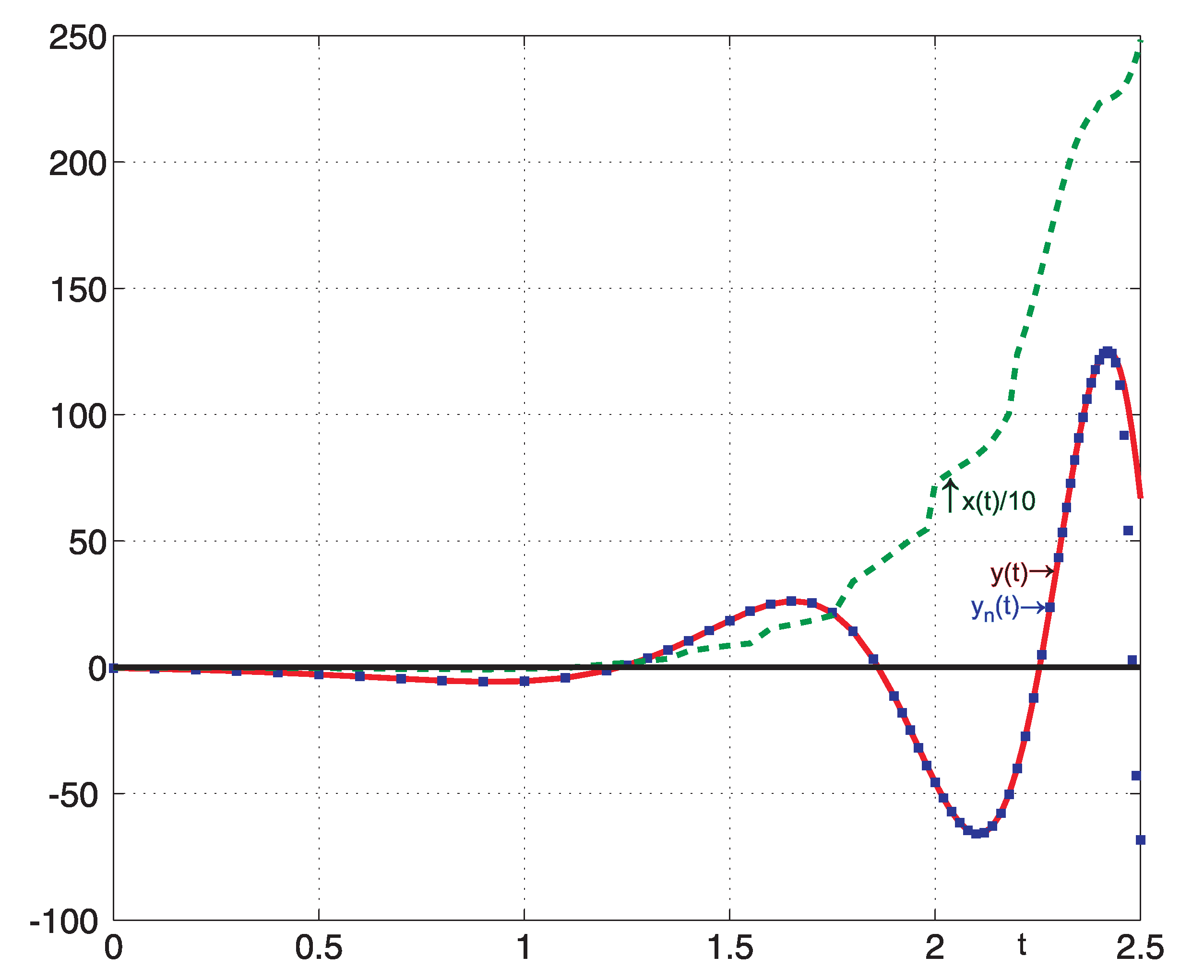
The recurrent solution is obtained based on Algorithm 3. Figure 1 shows the right hand-side $x\left(t\right)$, exact solution $y\left(t\right)$ and obtained solution $y_n\left(x\right)$ ([57], pp. 41–43). Moreover, the parameter p of the kernel $K(t,\tau )$ in the direct and inverse problems has slightly different values. As a result, the solution at $t\approx 2.5$ (with large fluctuation) differs markedly from the exact solution. Further, regularization should be applied to increase the stability of the solution.

Algorithm 3: Algorithm of the recurrent solution.

p=0.5; y1=x1; h2=t2-t1; h22=h2/2;

y2-h22*(K21*y1^2+K22*y2^2)=x2;

h22*K22*y2^2-y2+x2+h22*K21*y1^2=0; %quadratic equation for y2

y2=(1-\sqrt(1-2*h2*K22*(x2+h22*K21*y1^2)))/(h2*K22); %solution of QE

for i=3:N

yi-\sum_{j=2}^i hj/2*(K(i,j-1)*y(j-1)^2+Kij*yj^2)=xi;

hi2=hi/2; int=xi+hi2*K(i,i-1)*y(i-1)^2;

for j=2:i-1

int=int+hj/2*(K(i,j-1)*y(j-1)^2+Kij*yj^2);

end %j

hi2*Kii*yi^2-yi+int=0; %quadratic equation for yi

yi=(1-\sqrt(1-2*hi*Kii*int))/(hi*Kii); %solution of QE

end %i

5. Conclusions

The CESTAC method is among applicable and important methods to validate the numerical results based on the SA. For this aim, instead of usual applications such as Mathematica, Maple and Matlab the CADNA library should be run. Using this method and the CADNA library we can find the optimal iteration, the optimal approximation and the optimal error of numerical procedures. We introduced the stopping condition based on this method that it is independent from the exact solution. Also, using this condition we do not have the disadvantages of the traditional absolute error. Several theorems were proved to show the convergence of the ADM for solving linear and nonlinear VIE with discontinuous kernel. The main theorem of the CESTAC method was presented. Based on theorem we can apply the termination criterion (2) instead of (1). Several examples were solved by the ADM and the numerical results were validated using the CESTAC method. Also, we compared the results with numerical results obtained from the FPA.

References

1. Noeiaghdam, S.; Khoshrouye Ghiasi, E. An efficient method to solve the mathematical model of HIV infection for CD8+T cells. Int. J. Math. Model. Comput. 2019, 9, 267–281. [Google Scholar]
2. Naik, P.A.; Yavuz, M.; Zu, J. The Role of Prostitution on HIV Transmission with Memory: A Modeling Approach. Alex. Eng. J. 2020, 59, 2513–2531. [Google Scholar] [CrossRef]
3. Noeiaghdam, S.; Kamal Ali, K. Semi-analytical Method to Solve the Non-linear System of Equations to Model of Evolution for Smoking Habit in Spain. Int. J. Ind. Math. 2020, 12, 1377. [Google Scholar]
4. Noeiaghdam, S. Numerical Approximation of Modified Non-linear SIR Model of Computer Viruses. Contemp. Math. 2019, 1, 1. [Google Scholar] [CrossRef]
5. Noeiaghdam, S.; Sidorov, D. Caputo-Fabrizio Fractional Derivative to Solve the Fractional Model of Energy Supply-Demand System. Math. Model. Eng. Probl. 2020, 7, 359–367. [Google Scholar] [CrossRef]
6. Naik, P.A. Global dynamics of a fractional order SIR epidemic model with memory. Int. J. Biomath. 2020, 13, 2050071. [Google Scholar] [CrossRef]
7. Ahmad, A.; Farman, M.; Muhammad, F.; Naik, P.A.; Akgul, A.; Zafar, N.; Saleem, M.U. Modeling and numerical investigation of fractional-order bovine babesiosis disease. Numer. Methods Partial. Differ. Equ. 2020. [Google Scholar] [CrossRef]
8. Sidorov, D. Integral Dynamical Models. Singularities, Signals and Control. With a Foreword by H.-J. Reinhardt; World Scientific Series on Nonlinear Science; Series A: Monographs and Treatises, 87; World Scientific Publishing Co. Pte. Ltd.: Hackensack, NJ, USA, 2015. [Google Scholar] [CrossRef] [Green Version]
9. Sidorov, N.; Sidorov, D.; Sinitsyn, A. Toward General Theory of Differential-Operator and Kinetic Models; World Scientific Series on Nonlinear Science; Series A: Monographs and Treatises, 97; World Scientific Publishing Co. Pte. Ltd.: Hackensack, NJ, USA, 2020; p. 496. [Google Scholar] [CrossRef]
10. Sidorov, N.A.; Leontev, R.Y.; Dreglya, A.I. On small solutions of nonlinear equations with vector parameter in sectorial neighborhoods. Math. Notes 2012, 91, 90–104. [Google Scholar] [CrossRef]
11. Sidorov, D.N. Solvability of systems of volterra integral equations of the first kind with piecewise continuous kernels. Russ Math. 2013, 57, 54–63. [Google Scholar] [CrossRef]
12. Sidorov, D.; Muftahov, I.; Karamov, D.; Tomin, N.; Panasetsky, D.; Dreglea, A.; Liu, F.; Foley, A. A Dynamic Analysis of Energy Storage with Renewable and Diesel Generation using Volterra Equations. IEEE Trans. Ind. Inform. 2020, 16, 3451–3459. [Google Scholar] [CrossRef] [Green Version]
13. Sidorov, D.; Tynda, A.; Muftahov, I.; Dreglea, A.; Liu, F. Nonlinear Systems of Volterra Equations with Piecewise Smooth Kernels: Numerical Solution and Application for Power Systems Operation. Mathematics 2020, 8, 1257. [Google Scholar] [CrossRef]
14. Tynda, A.N.; Sidorov, D.N.; Muftahov, I.R. Numerical method for systems of nonlinear Volterra integral equations of the first kind with discontinuous kernels. Zhurnal SVMO 2018, 20, 55–63. [Google Scholar] [CrossRef] [Green Version]
15. Muftahov, I.; Tynda, A.; Sidorov, D. Numeric solution of Volterra integral equations of the first kind with discontinuous kernels. J. Comput. Appl. Math. 2017, 313, 119–128. [Google Scholar] [CrossRef]
16. Sidorov, D.N.; Zhukov, A.V.; Muftahov, I.R. Volterra equation based models for energy storage usage based on load forecast in EPS with renewable generation. Bull. Irkutsk State Univ. Ser. Math. 2018, 26, 76–90. [Google Scholar] [CrossRef]
17. Noeiaghdam, S.; Dreglea, A.; He, J.H.; Avazzadeh, Z.; Suleman, M.; Fariborzi Araghi, M.A.; Sidorov, D.; Sidorov, N. Error estimation of the homotopy perturbation method to solve second kind Volterra integral equations with piecewise smooth kernels: Application of the CADNA library. Symmetry 2020, 12, 1730. [Google Scholar] [CrossRef]
18. Noeiaghdam, S.; Sidorov, D.; Sizikov, V.; Sidorov, N. Control of accuracy on Taylor-collocation method to solve the weakly regular Volterra integral equations of the first kind by using the CESTAC method. Appl. Comput. Math. Int. J. 2020, 19, 81–105. [Google Scholar]
19. Noeiaghdam, S.; Sidorov, D.; Muftahov, I.; Zhukov, A.V. Control of Accuracy on Taylor–Collocation Method for Load Leveling Problem. Bull. Irkutsk State Univ. Ser. Math. 2019, 30, 59–72. [Google Scholar] [CrossRef]
20. Sidorov, N.A.; Sidorov, D.N. On the solvability of a class of Volterra operator equations of the first kind with piecewise continuous kernels. Math. Notes 2014, 96, 811–826. [Google Scholar] [CrossRef]
21. Muftahov, I.R.; Sidorov, D.N. Solvability and numerical solutions of systems of nonlinear Volterra integral equations of the first kind with piecewise continuous kernels. Bull. South Ural. State Univ. Ser. Math. Model. Program. Comput. Softw. 2016, 9, 130–136. [Google Scholar] [CrossRef]
22. Sizikov, V.; Sidorov, D. Generalized quadrature for solving singular integral equations of Abel type in application to infrared tomography. Appl. Numer. Math. 2016, 106, 69–78. [Google Scholar] [CrossRef] [Green Version]
23. Sidorov, D.N.; Sidorov, N.A. Convex majorants method in the theory of nonlinear Volterra equations. Banach J. Math. Anal. 2012, 6, 1–10. [Google Scholar] [CrossRef]
24. Micula, S. A Numerical Method for Weakly Singular Nonlinear Volterra Integral Equations of the Second Kind. Symmetry 2020, 12, 1862. [Google Scholar] [CrossRef]
25. Hashemizadeh, E.; Ebadi, M.A.; Noeiaghdam, S. Matrix method by Genocchi polynomials for solving nonlinear Volterra integral equations with weakly singular kernel. Symmetry 2020, 12, 2105. [Google Scholar] [CrossRef]
26. Davies, P.J.; Duncan, D.B. Numerical approximation of first kind Volterra convolution integral equations with discontinuous kernels. J. Integral Equ. Appl. 2017, 29, 41–73. [Google Scholar] [CrossRef] [Green Version]
27. Tikhonov, A.N.; Arsenin, V.Y. Solutions of Ill-Posed Problems; Wiley: New York, NY, USA, 1977; 258p. [Google Scholar]
28. Tikhonov, A.N.; Leonov, A.S.; Yagola, A.G. Nonlinear Ill-Posed Problems: Textbook; Course: Moscow, Russia, 2017; 400p. [Google Scholar]
29. Saelao, J.; Yokchoo, N. The solution of Klein-Gordon equation by using modified Adomian decomposition method. Math. Comput. Simul. 2020, 171, 94–102. [Google Scholar] [CrossRef]
30. González-Gaxiola, O. Numerical solution for Triki-Biswas equation by Adomian decomposition method. Optik 2019, 194, 163014. [Google Scholar]
31. Daoud, Y.; Khidir, A.A. Modified Adomian decomposition method for solving the problem of boundary layer convective heat transfer. Propuls. Power Res. 2018, 7, 231–237. [Google Scholar] [CrossRef]
32. Novin, R.; Fariborzi Araghi, M.A.; Mahmoudi, Y. A novel fast modification of the Adomian decomposition method to solve integral equations of the first kind with hypersingular kernels. J. Comput. Appl. Math. 2018, 343, 619–634. [Google Scholar] [CrossRef]
33. Mahmoudi, Y. A new modified Adomian decomposition method for solving a class of hypersingular integral equations of second kind. J. Comput. Appl. Math. 2014, 255, 737–742. [Google Scholar] [CrossRef]
34. Wazwaz, A.-M.; Rach, R.; Duan, J.-S. Adomian decomposition method for solving the Volterra integral form of the Lane–Emden equations with initial values and boundary conditions. Appl. Math. Comput. 2013, 219, 5004–5019. [Google Scholar] [CrossRef]
35. Bougoffa, L.; Mennouni, A.; Rach, R.C. Solving Cauchy integral equations of the first kind by the Adomian decomposition method. Appl. Math. Comput. 2013, 219, 4423–4433. [Google Scholar] [CrossRef]
36. Wazwaz, A.-M. Linear and Nonlinear Integral Equations, Methods and Applications; Higher Education Press: Beijing, China; Springer: Berlin/Heidelberg, Germany, 2011. [Google Scholar]
37. Wazwaz, A.-M. Partial Differential Equations and Solitary Waves Theory; Higher Education Press: Beijing, China; Springer: Berlin/Heidelberg, Germany, 2009. [Google Scholar]
38. Chesneaux, J.M. CADNA, an ADA tool for round–off error analysis and for numerical debugging. In Proceedings of the Congress on ADA, Aerospace, Barcelona, 20–25 May 1990. [Google Scholar]
39. Jézéquel, F.; Mecanique, C.R. A dynamical strategy for approximation methods. Comptes Rendus Mec. 2006, 334, 362–367. [Google Scholar] [CrossRef] [Green Version]
40. Chesneaux, J.M.; Jézéquel, F. Dynamical control of computations using the Trapezoidal and Simpson’s rules. J. Univers. Comput. Sci. 1998, 4, 2–10. [Google Scholar]
41. Vignes, J. Discrete Stochastic Arithmetic for Validating Results of Numerical Software. Spec. Issue Numer. Algorithms 2004, 37, 377–390. [Google Scholar] [CrossRef]
42. Vignes, J. A stochastic arithmetic for reliable scientific computation. Math. Comput. Simul. 1993, 35, 233–261. [Google Scholar] [CrossRef]
43. Graillat, S.; Jézéquel, F.; Wang, S.; Zhu, Y. Stochastic arithmetic in multi precision. Math. Comput. Sci. 2011, 5, 359–375. [Google Scholar] [CrossRef]
44. Graillat, S.; Jézéquel, F.; Picot, R. Numerical Validation of Compensated Summation Algorithms with Stochastic Arithmetic. Electron. Notes Theor. Comput. Sci. 2015, 317, 55–69. [Google Scholar] [CrossRef]
45. Fariborzi Araghi, M.A.; Noeiaghdam, S. Finding the optimal step of fuzzy Newton-Cotes integration rules by using CESTAC method. J. Fuzzy Set Valued Anal. 2017, 2, 62–85. [Google Scholar]
46. Fariborzi Araghi, M.A.; Noeiaghdam, S. Dynamical control of computations using the Gauss-Laguerre integration rule by applying the CADNA library. Adv. Appl. Math. Sci. 2016, 16, 1–18. [Google Scholar]
47. Noeiaghdam, S.; Fariborzi Araghi, M.A. Valid implementation of the Sinc-collocation method to solve the linear integral equations by CADNA library. J. Math. Model. 2019, 7, 63–84. [Google Scholar]
48. Noeiaghdam, S.; Fariborzi Araghi, M.A.; Abbasbandy, S. Finding optimal convergence control parameter in the homotopy analysis method to solve integral equations based on the stochastic arithmetic. Numer. Algorithms 2019, 81, 237–267. [Google Scholar] [CrossRef]
49. Noeiaghdam, S.; Fariborzi Araghi, M.A.; Abbasbandy, S. Valid implementation of Sinc-collocation method to solve the fuzzy Fredholm integral equation. J. Comput. Appl. Math. 2020, 370, 112632. [Google Scholar] [CrossRef]
50. Fariborzi Araghi, M.A.; Noeiaghdam, S. A valid scheme to evaluate fuzzy definite integrals by applying the CADNA library. Int. J. Fuzzy Syst. Appl. 2017, 6, 1–20. [Google Scholar] [CrossRef]
51. Noeiaghdam, S.; Fariborzi Araghi, M.A. A novel approach to find optimal parameter in the homotopy—Regularization method for solving integral equations. Appl. Math. Inf. Sci. 2020, 14, 1–8. [Google Scholar]
52. Noeiaghdam, S.; Sidorov, D.; Zamyshlyaeva, A.; Tynda, A.; Dreglea, A. A valid dynamical control on the reverse osmosis system using the CESTAC method. Mathematics 2021, 9, 48. [Google Scholar] [CrossRef]
53. Noeiaghdam, S.; Fariborzi Araghi, M.A. A novel algorithm to evaluate definite integrals by the Gauss-Legendre integration rule based on the stochastic arithmetic: Application in the model of osmosis system. Math. Model. Eng. Probl. 2020, 7, 577–586. [Google Scholar] [CrossRef]
54. Chesneaux, J.M. The equality relations in scientific computing. Numer. Algorithms 1994, 7, 129–143. [Google Scholar] [CrossRef]
55. El-kalla, I.L. Convergence of Adomian’s method applied to a class of Volterra type integro-differential equations. Int. J. Differ. Equ. Appl. 2005, 10, 225–234. [Google Scholar]
56. Sidorov, N.A. Parametrization of simple branching solutions of full rank and iterations in nonlinear analysis. Russian Math. 2001, 45, 55–61. [Google Scholar]
57. Verlan, A.F.; Sizikov, V.S. Integral Equations: Methods, Algorithms, Programs; Nauk. Dumka: Kiev, Ukraine, 1986. [Google Scholar]
Figure 1. Source function x ( t ) , exact solution y ( t ) and numerical solution y n ( t ) .
Mathematics 09 00260 g001