Article

On a Retarded Nonlocal Ordinary Differential System with Discrete Diffusion Modeling Life Tables

by
Francisco Morillas
1,* and
José Valero
2,*
1
Departament d’Economia Aplicada, Facultat d’Economia, Campus dels Tarongers s/n, Universitat de València, 46022 València, Spain
2
Centro de Investigación Operativa, Avda. Universidad s/n, Universidad Miguel Hernández de Elche, 03202 Elche, Spain
*
Authors to whom correspondence should be addressed.
Mathematics 2021, 9(3), 220; https://doi.org/10.3390/math9030220
Submission received: 21 December 2020 / Revised: 15 January 2021 / Accepted: 19 January 2021 / Published: 22 January 2021
(This article belongs to the Special Issue Mathematical Methods on Economic Dynamics)

Abstract

:
In this paper, we consider a system of ordinary differential equations with non-local discrete diffusion and finite delay and with either a finite or an infinite number of equations. We prove several properties of solutions such as comparison, stability and symmetry. We create a numerical simulation showing that this model can be appropriate to model dynamical life tables in actuarial or demographic sciences. In this way, some indicators of goodness and smoothness are improved when comparing with classical techniques.

1. Introduction

Nonlocal diffusion problems generated by convolution operators have been used widely in the literature in order to model diffusion processes. As explained in [1], a convolution operator can describe transport due to long-range dispersal mechanisms. Another application of such models is the approximation of reaction-diffusion equations, as done in [2] in the continuous case and in [3] in the discrete case. They have been also used to model phase transitions (see [4,5,6,7] among others). The long-time behavior of the solutions of such systems has been considered for example in [7,8]. In [9], the relation between a continuous nonlocal diffusion equation and its discrete counterpart was studied.
In our previous paper [10], we studied analytically and numerically the nonlocal ordinary differential system with discrete diffusion
d d t u i t = r D j i r u r t u i ( t ) + r Z \ D j i r g r t , i D , t > 0 , u i 0 = u i , 0 , i D ,
where D is a suitable subset of Z , showing that it is appropriate for modeling life tables. The main downside is that the predictions are only valid for a short term of about two or three years.
It seems, however, that some memory effects are present on life tables, so it would be better to consider a model with delay. This allows us to extend the validity of the predictions for larger periods of about five to ten years. Therefore, in this paper, we modify system (1) by means of the introduction of some delay terms. For life tables, the delay pattern is established via improvement rates [11]. We point out that our model is deterministic, non-parametric and predicts the evolution of the probability of death by age over time.
In Section 2, we study some properties of the solutions of the retarded nonlocal model such as a comparison principle, the stability of stationary points or the symmetry of solutions under certain assumptions. The analysis is carried out for a system with either a finite or an infinite number of equations, extending to the model with delay similar results from [10].
In Section 3, we apply the new model to life tables in Spain. We use the observed values in the period from 1908 to 2012 to fit the model and then validate it by making predictions in the period 2013–2018. We compare the predicted values with the observed ones by using two indicators of goodness. In both cases, the conclusion is that the model is appropriate for making quality predictions in the middle-term. We repeat the same calculations but using the Lee-Carter model, which is seminal and paradigmatic for this theory, obtaining that in almost all cases, our model improves the aforementioned indicators when comparing it with this classical model.

2. Properties of Solutions of Non-Local Diffusion Problems with Finite Delay

Let D be a subset of Z of one of the following types:
D = m 1 , m 1 + 1 , , m 2 , < m 1 < m 2 < + ,
D = Z ,
D = { i Z : i m } ,
D = { i Z : i m } , m Z .
For the cases (3)–(5), we define the Banach spaces
l 1 = { u i i D : sup i D u i < } , l 2 = { u i i Z \ D : sup i Z \ D u i < } , l 1 p = { u i i D : i D u i p < } , l 2 p = { u i i Z \ D : i Z \ D u i p < } ,
with the usual norms u l 1 = sup i D u i , u l 2 = sup i Z \ D u i , u l 1 p = i D u i p 1 p , u l 2 p = i Z \ D u i p 1 p . If D = Z , then l 1 = l , l 1 p = l p . In the case (2), the phase space is R m , m = m 2 m 1 + 1 , with its norm denoted by · R m . The scalar products in R m and l j 2 , j = 1 , 2 , will be given by · , · R m and · , · l j 2 , respectively.
We consider the following non-autonomous retarded problem with non-local diffusion:
d d t u i t = J ( t , u t ) i u i ( t ) , i D , t > τ , u i τ + s ϕ i s , i D , s [ h , 0 ] ,
where τ is the initial moment of time, and J : R + × C ( [ h , 0 ] , X ) X , with either X = R m , X = l 1 or X = l 1 1 , is the non-autonomous convolution operator defined by
J ( t , u t ) i = r D h 0 j i r u r ( t + s ) α i ( s ) d μ ( s ) + r Z \ D h 0 j i r g r t + s α i ( s ) d μ ( s ) , if i D ,
where u t = u i s i D , u t = u t + s for s [ h , 0 ] , j : Z R , g : R × Z \ D R and d μ ( s ) = ξ s d s being ξ · a probability density. We assume the following conditions:
H 1
j k 0 for all k Z .
H 2
i Z j i = 1 .
H 3
g C ( R , l 2 ) .
H 4
α i C ( [ h , 0 ] , R ) , α i s 0 for i D , s [ h , 0 ] .
Throughout the paper, the space C ( [ h , 0 ] , X ) will be denoted for short by C h and its supremum norm by · C h when no confusion arises. All the results in this section extend analogous ones from [10] in the same problem but without delay, that is, when h = 0 . In the case with delay we need to add conditions concerning the functions α i (see H 4 , H 5 , H 7 ).

2.1. A Finite Number of Equations

We assume now that D is given by (2), so X = R m .
Let us prove first the existence and uniqueness of solutions by applying the abstract theory for differential equations with delay [12].
Lemma 1.
Let ( H 1 ) ( H 4 ) hold. For any ϕ C ( [ h , 0 ] , R m ) and the initial moment τ, there exists a unique solution u · C 1 ( [ τ , + ) , R m ) of problem (6).
Proof. 
We write (6) in the form
d u d t = f u t + h ¯ t ,
where f u t = f m 1 u t , . . . , f m 2 ( u t ) T , h ¯ t = h m 1 t , . . . , h m 2 t T with
f i ( ϕ ) = r D h 0 j i r ϕ r ( s ) α i ( s ) d μ ( s ) ϕ i ( 0 ) , ϕ C h , h i t = r Z \ D h 0 j i r g r t + s α i ( s ) d μ ( s ) .
The map f : C h R m is globally Lipschitz continuous, which follows from
f ϕ 1 f ϕ 2 R m 2 i D r D h 0 j i r ϕ 1 r s ϕ 2 r s α i s d μ s + ϕ 1 i 0 ϕ 2 i 0 2 ϕ 1 ϕ 2 C h 2 i D h 0 α i s d μ s + 1 2 = C ϕ 1 ϕ 2 C h 2 .
On the other hand, the map h ¯ : [ τ , + ) R m is obviously continuous as g C ( R , l 2 ) .
Therefore, the map J : R × C h R m , J ( t , ϕ ) = f ϕ + h ¯ t , is jointly continuous in both variables and Lipschitz continuous on the second variable. Hence, Theorem 2.3 in [12] implies the existence of a unique solution u C ( [ τ h , t 0 ) , R m ) , defined at least for some t 0 > τ .
Since f is globally Lipschitz, it has sublinear growth, that is, there are constants C 1 , C 2 > 0 such that
f ϕ R m C 1 + C 2 ϕ C h for all ϕ C h .
Thus, it takes any bounded set of C h into a bounded set of R h . Since h is continuous, the map J takes closed bounded subsets of R × C h into bounded subsets of R m .
Let us prove that the solution exists for any t τ . If a solution u · were non-continuable on [ τ h , b ) , for any closed bounded set U in R × C h there would exists a time t U such that u t U for any t U t < b ([12], Theorem 3.2). We will obtain an estimate showing that the last is impossible for any solution.
Multiplying (7) by u and using (8) and g C ( R , l 2 ) we have
1 2 d d t u R m 2 C 1 + C 2 u t C h u t R m + h ¯ t R m u t R m C 3 + C 4 u t C h 2 for all τ t < b .
Integrating between τ and t + θ , τ t < b , θ [ h , 0 ] , t + θ τ , we obtain
u t + θ R m 2 u τ R m 2 + 2 C 3 b τ + 2 C 4 τ t + θ u s C h 2 d s .
Taking the supremum over θ [ h , 0 ] and taking into account that u t + θ R m ϕ C h if t + θ < τ , we get
u t C h 2 ϕ C h 2 + C 5 + C 6 τ t u s C h 2 d s .
Gronwall’s lemma implies that
u t C h 2 ϕ C h 2 + C 5 e C 6 t τ for all τ t < b .
Let B 0 be the closed ball in C h centered at 0 with radius R = 2 ϕ C h 2 + C 5 e C 6 ( b τ ) and put U = [ τ , b ] × B 0 . Then, if u · were non-continuable, there would exist t U such that u t U for any t U t < b . This contradicts (9).
Finally, we prove that u · C 1 ( [ τ , + ) , R m ) . We have seen that h ¯ : [ τ , + ) R m is a continuous function. Additionally, f : C h R m is globally Lipschitz and u C ( [ h , + ) , R m ) , so u t C ( [ 0 , + ) , C h ) . Hence, the application t f u t + h ¯ t , t τ , is a continuous function, so using the equality (7), we obtain that d u d t is also continuous on [ τ , + ) . □
Further, we will prove that the solutions are non-negative if the initial condition is non-negative. This result implies in turn a comparison principle.
For an arbitrary (real) constant v, we denote v + = max { 0 , v } , v = max { 0 , v } . We observe that v = v + v and that v· v + = v + 2 .
Proposition 1.
Let ( H 1 ) ( H 4 ) hold. Assume that g r t 0 for any t , r R × Z \ D . Let ϕ C h , 0 , R n be such that ϕ i s 0 for s h , 0 , i D . Then, the solution u · of problem (6) satisfies that u i t 0 for all i D , t τ .
Proof. 
Multiplying the equation in (6) by u + and using the equality ([13], Lemma 2.2)
d u d t , u + R m = 1 2 d d t u + R m 2
we have
1 2 d d t u t + R m 2 = i D r D h 0 ( u r t + s ) ( u i t ) + j i r α i s d μ s r Z \ D h 0 j i r g r t + s ( u i t ) + α i s d μ s u t + R m 2 ,
and discarding the negative terms
1 2 d d t u t + R m 2 i D r D h 0 ( u r t + s ) ( u i t ) + j i r α i s d μ s = i D r D h 0 ( u r t + s ) + ( u r t + s ) ( u i t ) + j i r α i s d μ s i D r D h 0 ( u r t + s ) + ( u i t ) + j i r α i s d μ s 1 2 i D r D h 0 ( u r t + s ) + 2 + ( u i t ) + 2 j i r α i s d μ s .
We deduce by H 2 that
1 2 d d t u t + R m 2 u t + C h 2 i D h 0 r D j i r α i s d μ s M u t + C h 2 ,
where M = i D h 0 α i s d μ s . Integrating over τ , t we find
u t + R m 2 u τ + R m 2 + 2 M τ t u s + C h 2 d s .
Taking t = t + θ for θ h , 0 , t + θ τ , and using that u t + θ + R m = ϕ ( t + θ ) + R m if t + θ < τ the last expression reads as
u t + θ + R m 2 ϕ + C h 2 + 2 M τ t + θ u s + C h 2 d s ,
and taking the supremum over [ h , 0 ] ,
u t + C h 2 ϕ + C h 2 + 2 M τ t u s + C h 2 d s .
Finally, Gronwall’s lemma gives
u t + C h 2 ϕ + C h 2 e 2 M t τ ,
so u t 0 for all t τ .  □
Corollary 1.
Let ( H 1 ) ( H 4 ) hold. Additionally, let ϕ 1 , ϕ 2 be two initial conditions such that ϕ 1 ϕ 2 in C h , 0 , R n , and let g 1 , g 2 C R , l 2 be two functions such that g 1 ( t ) g 2 ( t ) for all t τ . We consider the solutions u ( ·), v ( ·) of problem (6) with ϕ = ϕ 1 , g = g 1 and ϕ = ϕ 2 , g = g 2 , respectively. Then, u ( t ) v ( t ) for all t τ .
Let us consider the autonomous case, that is, the function g does not depend on t. Assume also that α does not depend on i and denote
M 1 = M 1 ( h ) = h 0 α ( s ) d μ ( s ) .
A fixed point u R m has to satisfy the following system:
M 1 r D j i r u r + u i = M 1 r Z \ D j i r g r = b i , i D .
We can rewrite it in the matrix form
A u = b ,
where
A = I M 1 j 0 j 1 j 2 j m 1 m 2 j 1 j 0 j 1 j 2 j m 1 m 2 + 1 j 2 j 1 j 0 j 1 j m 1 m 2 + 2 j m 2 m 1 1 j 2 j 1 j 0 j 1 j m 2 m 1 j 2 j 1 j 0 .
We consider the following condition:
M 1 r D j i r < 1 , i D .
Let r i be the sum of the elements of the row i of the matrix A. Then, (11) implies that
r i = 1 M 1 r D j i r > 0 .
Hence, A is diagonal dominant, so that the system has a unique solution, i.e., there exists a unique fixed point u ¯ .
We will show that it is stable. For this aim, we need to study the properties of the solutions of the homogeneous system
d d t v i t = r D h 0 j i r v r ( t + s ) α ( s ) d μ ( s ) v i ( t ) , i D , t > 0 , v i s ϕ i s , i D , s [ h , 0 ] .
We recall the definition of stability of stationary points.
Definition 1.
The zero solution of (12) is stable in the sense of Lyapunov if for each ϵ > 0 there exists γ ϵ > 0 such that if v 0 R m < γ , then v t R m < ϵ t 0 . Additionally, we say that 0 is asymptotically stable if it is stable and there is γ > 0 such that if v 0 R m < γ , then l i m t + v t R m = 0 . It is exponentially stable if it is stable and, moreover, there exist γ , c 0 , λ > 0 such that if v 0 R m < γ , then v t R m c 0 e λ t for all t 0 .
Lemma 2.
Let ( H 1 ) ( H 4 ) hold. Assume that (11) holds and that h < 1 2 log 1 δ ( h ) , where
δ ( h ) = min i D { 1 M 1 ( h ) r D j i r } = min r D { 1 M 1 ( h ) i D j i r } .
Then, the zero solution of problem (12) is exponentially stable (hence, asymptotically stable). Moreover, it attracts uniformly as t + any solution starting on a bounded set.
Remark 1.
Although the condition h < 1 2 log 1 δ ( h ) is an inequation, it is easy to see that for h small enough it holds true. Indeed, we can choose first h 0 > 0 such that M 1 ( h 0 ) r D j i r < 1 for any i D , which implies that M 1 ( h ) r D j i r < 1 for all h h 0 , i D . Then, we choose h h 0 such that h < 1 2 log 1 δ ( h 0 ) 1 2 log 1 δ ( h ) , where we have used that δ ( h ) is a non-increasing function.
Proof. 
Let v t be an arbitrary solution to problem (12) with ϕ C h d .
Let 0 < λ < 2 . Then
d d t e λ t v R m 2 = λ e λ t v ( t ) R m 2 + 2 e λ t i D v i ( t ) r D h 0 j i r v r ( t + s ) α ( s ) d μ ( s ) v i ( t ) = λ 2 e λ t v ( t ) R m 2 + 2 e λ t i D v i ( t ) r D h 0 j i r v r ( t + s ) α ( s ) d μ ( s ) .
We estimate the last term as follows:
2 e λ t i D v i ( t ) r D h 0 j i r v r ( t + s ) α ( s ) d μ ( s ) 2 e λ t M 1 ( h ) 2 i D r D j i r v i ( t ) 2 + 1 2 i D r D h 0 j i r v r ( t + θ ) 2 α ( s ) d μ ( s ) 2 e λ t M 1 ( h ) 2 i D v i ( t ) 2 r D j i r + 1 δ h 2 M 1 h h 0 r D v r ( t + θ ) 2 α ( s ) d μ ( s ) = 1 δ h e λ t i D v i ( t ) 2 + sup θ [ h , 0 ] r D v r ( t + θ ) 2 .
Hence,
d d t e λ t v R m 2 λ 2 e λ t v ( t ) R m 2 + 2 e λ t 1 δ ( h ) v t C h 2 2 e λ t 1 δ ( h ) v t C h 2 .
Integrating over 0 , t , we have
e λ t v ( t ) R m 2 v 0 R m 2 + 2 1 δ ( h ) 0 t e λ s v s C h 2 d s .
We set t + θ , t + θ 0 , instead of t and obtain that
v ( t + θ ) R m 2 e λ ( t + θ ) v 0 R m 2 + 2 1 δ ( h ) e λ ( t + θ ) 0 t + θ e λ s v s C h 2 d s e λ t e λ h v 0 R m 2 + 2 1 δ ( h ) e λ t e λ h 0 t e λ s v s C h 2 d s .
Thus, as v ( t + θ ) R m ϕ C h 2 for t + θ < 0 , we have
e λ t v t C h 2 e λ h ϕ C h 2 + 2 1 δ ( h ) e λ h 0 t e λ s v s C h 2 d s .
By Gronwall’s lemma, we get
e λ t v t C h 2 e λ h ϕ C h 2 e 2 1 δ ( h ) e λ h t ,
so
v t C h 2 e λ h ϕ C h 2 e 2 1 δ ( h ) e λ h λ t .
Condition h < 1 2 log 1 δ ( h ) implies that 2 1 δ ( h ) e 2 h < 2 , so there exists 0 < λ * < 2 such that 2 1 δ ( h ) e λ * h = λ * . Therefore, choosing λ λ * , 2 we obtain that 2 1 δ ( h ) e λ h λ < 0 . It follows from inequality (13) that 0 is exponentially stable and that it attracts uniformly as t + any solution starting on a bounded set. □
Corollary 2.
Let ( H 1 ) ( H 4 ) hold. We consider equation (6) in the autonomous case, that is, the function g does not depend on t and τ = 0 . Assume that (11) holds and that h < 1 2 log 1 δ ( h ) . Then, the fixed point u ¯ is exponentially stable for the autonomous problem (6). Moreover, it uniformly attracts every solution starting on a bounded set.
We finish this subsection by showing that symmetry of the initial condition and the functions g , α and j imply symmetry of the solution.
Lemma 3.
Let ( H 1 ) ( H 4 ) hold. Let D = { d , d + 1 , . . . , 0 , . . . , d 1 , d } , d N . Assume also that g i t = g i t , for all i Z \ D , t τ , j i = j i , α i s = α i s , ϕ i ( s ) = ϕ i ( s ) for any i Z , s [ h , 0 ] . Then, the unique solution to problem (6) is symmetric, that is,
u i ( t ) = u i ( t ) for all i D , t τ h .
Proof. 
Let w i t = u i t . Then, the hypothesis of the lemma implies that
d w i d t = d u i d t = r D h 0 j i r u r ( t + s ) α i ( s ) d μ ( s ) + r Z \ D h 0 j i r g r t + s α i ( s ) d μ ( s ) u i t = r D h 0 j i + r w r ( t + s ) α i ( s ) d μ ( s ) + r Z \ D h 0 j i + r g r t + s α i ( s ) d μ ( s ) w i t = r D h 0 j i r ¯ w r ¯ ( t + s ) α i ( s ) d μ ( s ) + r Z \ D h 0 j i r ¯ g r ¯ t + s α i ( s ) d μ ( s ) w i t
and w i τ + s = u i τ + s = u i τ + s = ϕ i ( s ) for s [ h , 0 ] . It follows that w · is the unique solution to problem (6) with initial condition ϕ . Hence, w i t = u i t = u i t for all i D and t τ h .  □

2.2. An Infinite Number of Equations

We consider now the case where the system can admit an infinite number of equations. For this we define D as a subset of Z of one of the types given in (3)–(5).
First, we study the Equation (6) with X = l 1 , so J : R × l 1 l 1 .
We will need the following extra assumption:
H 5
sup i D h 0 α i s d μ s < .
Remark 2.
Conceptually, in life tables, it can be of interest to use an infinite number of equations. For example, domains of type (5) can be used for the biometric function Life Expectancy, which is defined (at year t) as i = 0 p i t · i , where p i t represents the survival probability at age i at year t. We note that in this work we use the function q i = 1 p i , where q i represents the risk of death at age i. In Section 3.1.2, we apply model (6) with an infinite number of equations to the variable q i .
In order to obtain the existence and uniqueness of solutions we use once again the abstract theory for differential equations with delay given in ([12], Chapter 2). Although the results are stated in the phase space R n , the theorems are valid for a Banach space as well.
Lemma 4.
Assume that, in addition to ( H 1 ) ( H 4 ) , ( H 5 ) is satisfied. Then, for any ϕ C ( [ h , 0 ] , l 1 ) there exists a unique solution u · C 1 ( [ τ , + ) , l 1 ) of problem (6).
Proof. 
We proceed as in Lemma 1. System (6) is considered in the form (7), where in this case f i u t i D and h i t i D are column vectors with infinite elements.
We prove first that the map f : l 1 l 1 is globally Lipschitz continuous. Indeed, by (H2) and (H5), we have
f ϕ 1 f ϕ 2 l 1 2 sup i D r D h 0 j i r ϕ 1 r s ϕ 2 r s α i s d μ s + ϕ 1 i 0 ϕ 2 i 0 sup s [ h , 0 ] , i D ϕ 1 i s ϕ 2 i s sup i D r D h 0 j i r α i s d μ s + 1 ϕ 1 ϕ 2 C ( [ h , 0 ] , l 1 ) sup i D r D j i r h 0 α i s d μ s + 1 ϕ 1 ϕ 2 C ( [ h , 0 ] , l 1 ) sup i D h 0 α i s d μ s + 1 .
Second, we check that h ¯ t is a continuous map for the cases (4) and (5). If t n t in R , then by H 3 we obtain that
h ¯ t n h ¯ t l 1 = sup i D r Z \ D h 0 j i r g r t n + s α i ( s ) d μ ( s ) r Z \ D h 0 j i r g r t + s α i ( s ) d μ ( s ) sup i D r Z \ D h 0 j i r g r t n + s g r t + s α i ( s ) d μ ( s ) sup s [ h , 0 ] , i D g i t n + s g i t + s sup i D r Z \ D j i r h 0 α i ( s ) d μ ( s ) g t n g t C ( [ h , 0 ] , l 2 ) sup i D h 0 α i ( s ) d μ ( s ) 0 as n .
In order to prove that the solution is globally defined for t τ , we need to obtain an estimate of its growth. Let b > τ be the maximal time of existence of the solution u · , so it is not continuable in [ τ h , b ). Since f is Lipschitz, it has sublinear growth, and h · is bounded in [ τ h , b ] . Hence,
d u d t l 1 K 1 + K 2 u t C ( [ h , 0 ] , l 1 ) , for t [ τ h , b ) ,
so
u t l 1 u τ l 1 + τ t d u d r l 1 d r u τ l 1 + K 1 b τ + K 2 τ t u r C ( [ h , 0 ] , l 1 ) d r ,
for t [ τ h , b ) . Arguing as in the proof of Lemma 1 we deduce that
u t C ( [ h , 0 ] , l 1 ) ϕ C ( [ h , 0 ] , l 1 ) + K 1 b τ e K 2 t τ .
Again by the same arguments of the proof of Lemma 1, we arrive at a contradiction. □
Further, we will obtain a comparison principle as in Proposition 1. For this aim, we need two additional assumptions:
H 6
There exist K > 0 and a l 1 2 such that a i > 0 , for all i D , and
i D a i 2 a r 2 j i r K for every r D .
H 7
There exists α · C ( [ h , 0 ] , R ) such that α i s α s for all s [ h , 0 ] .
It is obvious that H 7 is stronger than H 5 . Condition (H6) is satisfied for any kernel j i with subexponential growth, that is, j i c e α i for some α , c > 0 [10].
Proposition 2.
Let H 1 H 4 , H 6 ( H 7 ) hold. Assume that g r t 0 for any t , r R × Z \ D . Let ϕ C h , 0 , l 1 be such that ϕ i s 0 for s h , 0 and i D . Then, u i t 0 for all i D , t τ .
Proof. 
We define the function v t = v i t i D = a i u i t i D , which belongs to C 1 [ τ , ) , l 1 2 as a l 1 2 . We know by ([13], Lemma 2.2) that
d v d t , v + l 1 2 = 1 2 d d t v + l 1 2 2 .
The function v satisfies the equality
d v i d t = a i r D h 0 j i r u r ( t + s ) α i ( s ) d μ ( s ) a i r Z \ D h 0 j i r g r t + s α i ( s ) d μ ( s ) + v i t .
Multiplying it by v + , we have
1 2 d d t v t + l 1 2 2 = i D r D h 0 ( u r t + s ) ( v i t ) + a i j i r α i s d μ s r Z \ D h 0 a i j i r g r t + s ( v i t ) + α i s d μ s v t + 2 i D r D h 0 ( u r t + s ) + ( v i t ) + a i j i r α i s d μ s 1 2 i D r D h 0 ( v r t + s ) + 2 a i 2 a r 2 j i r α i s d μ s + 1 2 i D r D h 0 ( v i t ) + 2 j i r α i s d μ s .
Making use of (H7), the last term is estimated by
1 2 i D r D h 0 ( v i t ) + 2 j i r α i s d μ s 1 2 i D ( v i t ) + 2 h 0 α i s d μ s 1 2 h 0 α s d μ s v t + l 1 2 2 .
By (H6) and (H7), for the penultimate term, we obtain
1 2 i D r D h 0 ( v r t + s ) + 2 a i 2 a r 2 j i r α i s d μ s 1 2 r D i D a i 2 a r 2 j i r h 0 ( v r t + s ) + 2 α s d μ s K 2 h 0 r D ( v r t + s ) + 2 α s d μ s K 2 v t + C ( [ h , 0 ] , l 1 2 ) 2 h 0 α s d μ s .
Since i D a i 2 a r 2 j i r h 0 ( v r t + s ) + 2 α s d μ s is convergent for each r D and the iterated limit
r D i D a i 2 a r 2 j i r h 0 ( v r t + s ) + 2 α s d μ s
is convergent as well, the change of order in the summatories is justified. Furthermore, v t C [ h , 0 ] , l 1 2 implies that S k = r D , r k ( v r t + s ) + 2 α s converges to r D ( v r t + s ) + 2 α s uniformly in s [ h , 0 ] , so it is correct to change the order of the summatory and the integral in the penultimate inequality of (15).
Thus, there exists a constant M > 0 satisfying
v t + l 1 2 2 v τ + l 1 2 2 + M τ t v s + C ( [ h , 0 ] , l 1 2 ) 2 d s .
Arguing as in the proof of Proposition 1 it follows that u t 0 for all t τ .  □
Corollary 3.
Assume the conditions of Proposition 2. Let ϕ 1 , ϕ 2 be two initial conditions such that ϕ 1 ϕ 2 in C h , 0 , l 1 , and let g 1 , g 2 C R , l 2 be two functions such that g 1 ( t ) g 2 ( t ) for all t τ . We consider the solutions u ( ·), v ( ·) of the problem (6) with ϕ = ϕ 1 , g = g 1 and ϕ = ϕ 2 , g = g 2 , respectively. Then, u ( t ) v ( t ) for all t τ .
Second, we study the equation (6) with X = l 1 1 , so J : R × l 1 1 l 1 1 if we replace condition (H3) by
H 3 b
g C ( R , l 2 1 ) .
Lemma 5.
Assume that conditions (H1), (H2), (H3b), (H4) and (H7) are satisfied. Then, for any ϕ C ( [ h , 0 ] , l 1 1 ) there exists a unique solution u · C 1 ( [ τ , + ) , l 1 1 ) of problem (6).
Proof. 
As in Lemma 4, we only need to check that f : l 1 1 l 1 1 is globally Lipschitz continuous and that h ¯ : R l 1 1 is a continuous map for the cases (4) and (5).
By (H2) and (H7), we have
f ϕ 1 f ϕ 2 l 1 1 2 i D r D h 0 j i r ϕ 1 r s ϕ 2 r s α i s d μ s + ϕ 1 i 0 ϕ 2 i 0 r D i D j i r h 0 ϕ 1 r s ϕ 2 r s α s d μ s + ϕ 1 0 ϕ 2 0 l 1 1 h 0 r D ϕ 1 r s ϕ 2 r s α s d μ s + ϕ 1 0 ϕ 2 0 l 1 1 ϕ 1 ϕ 2 C ( [ h , 0 ] , l 1 1 ) h 0 α s d μ s + 1 .
If t n t in R , then by (H3b) and (H7), we obtain that
h ¯ t n h ¯ t l 1 1 = i D r Z \ D h 0 j i r g r t n + s α i ( s ) d μ ( s ) r Z \ D h 0 j i r g r t + s α i ( s ) d μ ( s ) r Z \ D i D j i r h 0 g r t n + s g r t + s α ( s ) d μ ( s ) h 0 r Z \ D g r t n + s g r t + s α ( s ) d μ ( s ) g t n g t C ( [ h , 0 ] , l 2 1 ) h 0 α ( s ) d μ ( s ) 0 as n .
The change of the order in the summatories is justified in the same way as in Lemma 2. On the other hand, since the functions l 1 · = { g r t n + · g r t + · α s } r D , l 2 · = { ϕ 1 r s ϕ 2 r s α s } r D belong to C ( [ h , 0 ] , l 2 1 ) and C ( [ h , 0 ] , l 1 1 ) respectively, by a standard compactness argument, we obtain that the sequences S k 1 = r Z \ D , r > k g r t n + s g r t + s α s converge uniformly in s [ s , 0 ] to r Z \ D g r t n + s g r t + s α s , as k , and the sequence S k 2 = r Z \ D , r > k ϕ 1 r s ϕ 2 r s α s converges uniformly to r Z \ D ϕ 1 r s ϕ 2 r s α s . Thus, in both cases, the limit function is integrable and it is legitimate to change the order of the summatory and the integral. □
We study the comparison principle also in this case.
Proposition 3.
Suppose that conditions (H1), (H2), (H3b), (H4) and (H7) are satisfied. Assume that g r t 0 for any t , r R × Z \ D . Let ϕ C h , 0 , l 1 1 be such that ϕ i s 0 for s h , 0 and i D . Then, u i t 0 for all i D , t τ .
Proof. 
As u C 1 [ τ , + ) , l 1 1 C 1 [ τ , + ) , l 1 2 , we obtain arguing as in Proposition 2 that
1 2 d d t u t + l 1 2 2 i D r D h 0 ( u r t + s ) + ( u i t ) + j i r α i s d μ s 1 2 i D r D h 0 ( u r t + s ) + 2 j i r α i s d μ s + 1 2 i D r D h 0 ( u i t ) + 2 j i r α i s d μ s .
Condition (H7) implies as in (14) and (15) that
1 2 i D r D h 0 ( u i t ) + 2 j i r α i s d μ s 1 2 h 0 α s d μ s u t l 1 2 2 ,
1 2 i D r D h 0 ( u r t + s ) + 2 j i r α i s d μ s 1 2 r D i D j i r h 0 ( u r t + s ) + 2 α s d μ s 1 2 h 0 r D ( u r t + s ) + 2 α s d μ s 1 2 u t + C h 2 h 0 α s d μ s .
The proof is finished in the same way as in Proposition 2. □
Corollary 4.
Assume the conditions of Proposition 3. Let ϕ 1 , ϕ 2 be two initial conditions such that ϕ 1 ϕ 2 in C h , 0 , l 1 1 , and let g 1 , g 2 C R , l 2 be two functions such that g 1 ( t ) g 2 ( t ) for all t τ . We consider the solutions u ( ·), v ( ·) of the problem (6) with ϕ = ϕ 1 , g = g 1 and ϕ = ϕ 2 , g = g 2 , respectively. Then, u ( t ) v ( t ) for all t τ .
We finish this section by showing that if D = Z and the initial condition and the functions j i , α i and the initial condition are symmetric, then the solution is symmetric well.
Lemma 6.
Let either the conditions of Lemma 4 or 5 hold and let D = Z . Assume that j k = j k , ϕ k s = ϕ k s , α k s = α k s for all k D , s [ h , 0 ] . Then, the unique solution given in Lemmas 4 and 5 satisfies:
u k t = u k t for all k D , t τ h .
Proof. 
The proof follows the same lines as in Lemma 3 except that the term containing the function g is now missing. □

3. Application to Life Tables

Life tables are a widely used tool in demographic sciences or in actuarial field to study the behavior of a population in relation to the survival, or mortality, in a region or in a period of time. The implications of the results derived from them have a great importance, for example, for the analysis of the sustainability of the pension system; for the comparison of populations via indicators as expectation of life; for the estimation of the insurance premium; or for the calculation of the mathematical reserves to guarantee the pay of the claims [14].
Life tables are structured in biometric functions and the relations between them (see, for example, [15,16,17]). Some of these important functions, among others, can be: the survival probability at exact age x, p x , or its complement, the probability of death, q x (the focus of this work); the expectation of life at concrete age x, e x ; the central rate of mortality by age, m x , etc. Usually, we do not know the true values of the biometric functions and, then, they are treated as underlying values, which are unknown. In this situation, these values can be approximated using techniques or methodologies from this field of knowledge (see, [18], https://www.mortality.org/Public/Docs/MethodsProtocol.pdf or [19], among others). In this work, as in our previous paper [10], the aim is to estimate and predict the true probabilities of death (at each age x). In general, in order to estimate the values of a biometric function, different points of view and several types of techniques can be used. We consider three important paradigms: a first classification between the stochastic and the non-stochastic paradigms; second, we distinguish the situations when the model is based on the parametric point of view or, on the contrary, it does not consider parameters; finally, in the third level, we differentiate between the dynamic point of view (if the model considers the evolution with time) or the static point of view (the changes with time are not considered). The difference between the stochastic and non-stochastic frameworks is based, in actuarial practice, on the use or the interpretation of the results of the technique. For example, the Gompertz law [20] can be used in a deterministic framework (the results of the fit of the Gompertz law are used as unique values and as input in other steps of the process as, for example, in tarification) or it can be used in a stochastic framework, for example, by considering the fit as a realization of the random process of interest. The literature on this topic is extensive. The papers [11,15] contain a good introduction to the stochastic framework. The works of [21,22] introduce us to parametric and non parametric models. The works [16,23,24,25,26] allow us to know examples of stochastic, parametric and statics models. Concerning stochastic, parametric and dynamical models, the works [27,28,29,30,31] are interesting. We can find examples of stochastic, nonparametric and static models in [32,33,34,35]; for non-parametric and dynamical models, see [36].
As in the previous work [10], in this paper, we consider a non-stochastic paradigm, with a non-parametric model and a dynamical point of view. However, in this work, we consider the previous information as well. Thus, the difference between these two works is the use of the past information, via improvement rates. In the paper [10], history is not considered, and only the current (actual) data are used to estimate the predictions for the future. That procedure has the important limitation that the predictions are only valid for a short term, for periods of two or three years. The technique that is proposed in this work avoids this limitation and, by considering the history of the mortality rates, improves the previous results because it allows us to make predictions for periods of five to ten years.
In order to introduce the previous information, we establish a delay pattern via improvement rates [11].

3.1. Dynamical Kernel Graduation with Delay

In order to improve the dynamical model (1), which was proposed in [10], in this work, we introduce the history using the concept of Improvement Rate (see [37,38,39,40]). These rates characterize the evolution of the mortality year-to-year or between two arbitrary moments, t 0 and t 1 . In this sense, we use the classical definition of improvement rate between t 0 and t 1 ( t 0 < t 1 ) at age x, given by r x t 0 , t 1 = q x t 1 / q x t 0 . If we consider as delay the value d = t 1 t 0 > 0 , then, r x t 0 , t 1 r x t 0 , t 0 + d . Similarly, we define the global improvement rate between t 0 and t 1 , r ¯ t 0 , t 1 , as the coefficient of the linear model without constant term of the observed death rates, that is, we fit the linear model
q · t 1 = r ¯ t 0 , t 1 · q · t 0
with the data q 0 t 0 , , q ω t 0 and q 0 t 1 , , q ω t 1 .

3.1.1. Procedure by Steps

The proposed method can be summarized as follows:
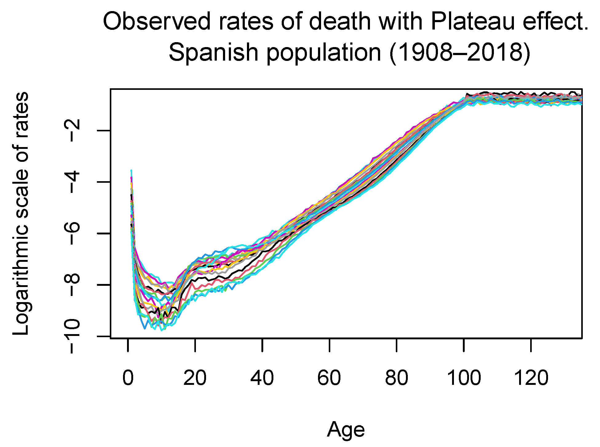
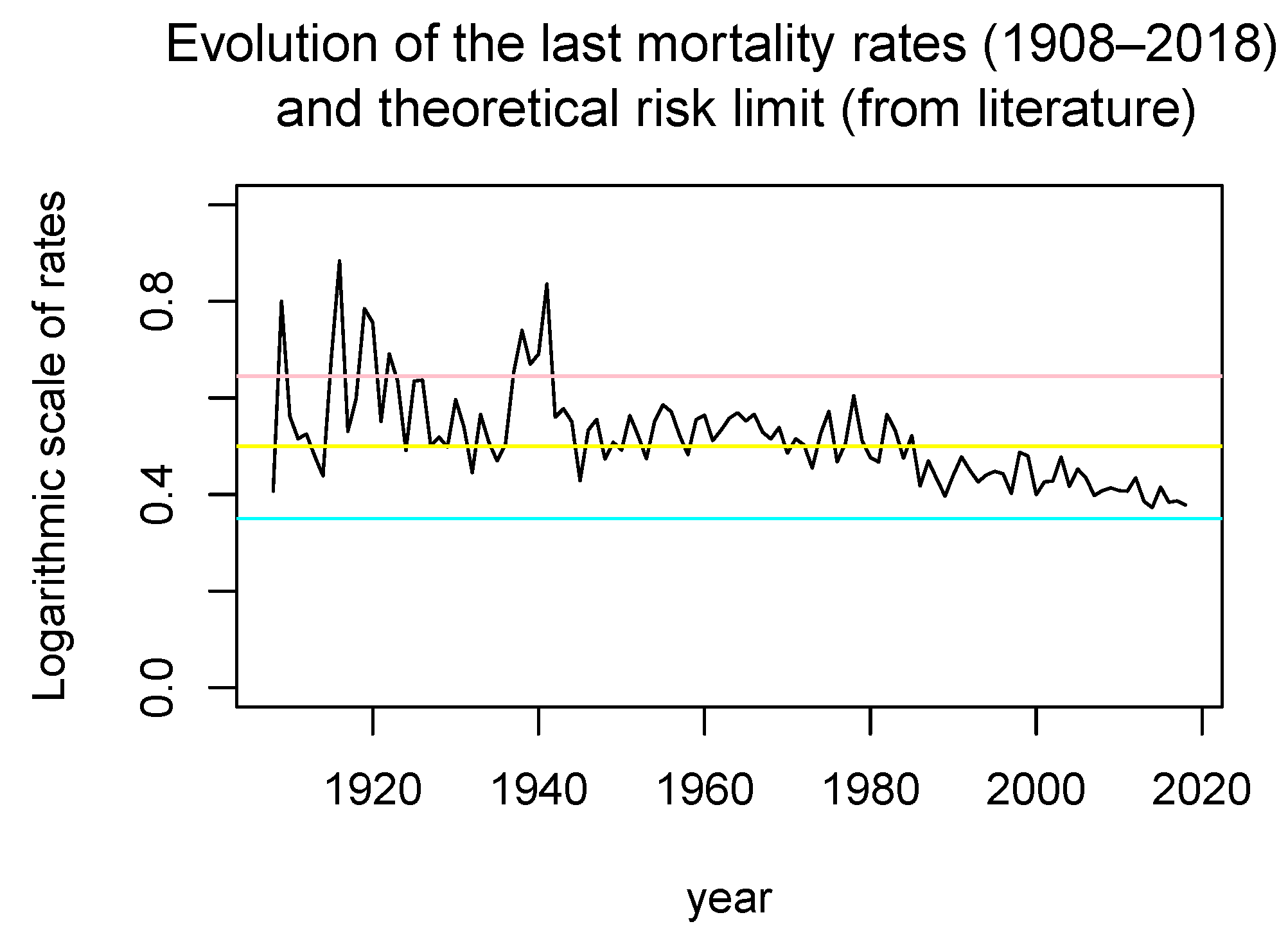
  • We consider the observed mortality rates at each age (from 0 to 100) and each year in the considered period (from 1908 to 2019), and denote them by q x t , x D =   0 , , 100 , t   1908 , , 2019 . Additionally, we consider the values of g x t , which is the rate of death either at “negative ages” or after the actuarial infinite (we have chosen it to be equal to 100).
  • We estimate the improvement rates by age and delays, that is:
    y e a r d e l a y 1 2 3 4 . . . r ¯ 1908 1909 q · 1909 q · 1908 r ¯ 1908 1910 q · 1910 q · 1908 r ¯ 1908 1911 q · 1911 q · 1908 r ¯ 1908 1912 q · 1912 q · 1908 r ¯ 1908 2017 q · 2017 q · 1908 r ¯ 1908 2018 q · 2018 q · 1908 r ¯ 1909 1910 q · 1910 q · 1909 r ¯ 1909 1911 q · 1911 q · 1909 r ¯ 1909 1912 q · 1912 q · 1909 r ¯ 1909 1913 q · 1913 q · 1909 r ¯ 1909 2017 q · 2017 q · 1909 r ¯ 1910 1911 q · 1911 q · 1910 r ¯ 1910 1912 q · 1912 q · 1910 r ¯ 1910 1913 q · 1913 q · 1910 r ¯ 1910 1914 q · 1914 q · 1910 r ¯ 1911 1912 q · 1912 q · 1911 r ¯ 1911 1913 q · 1913 q · 1911 r ¯ 1911 1914 q · 1914 q · 1911 r ¯ 1911 1915 q · 1915 q · 1911 r ¯ 2016 2017 q · 2017 q · 2016 r ¯ 2016 2018 q · 2018 q · 2016 r ¯ 2017 2018 q · 2018 q · 2017
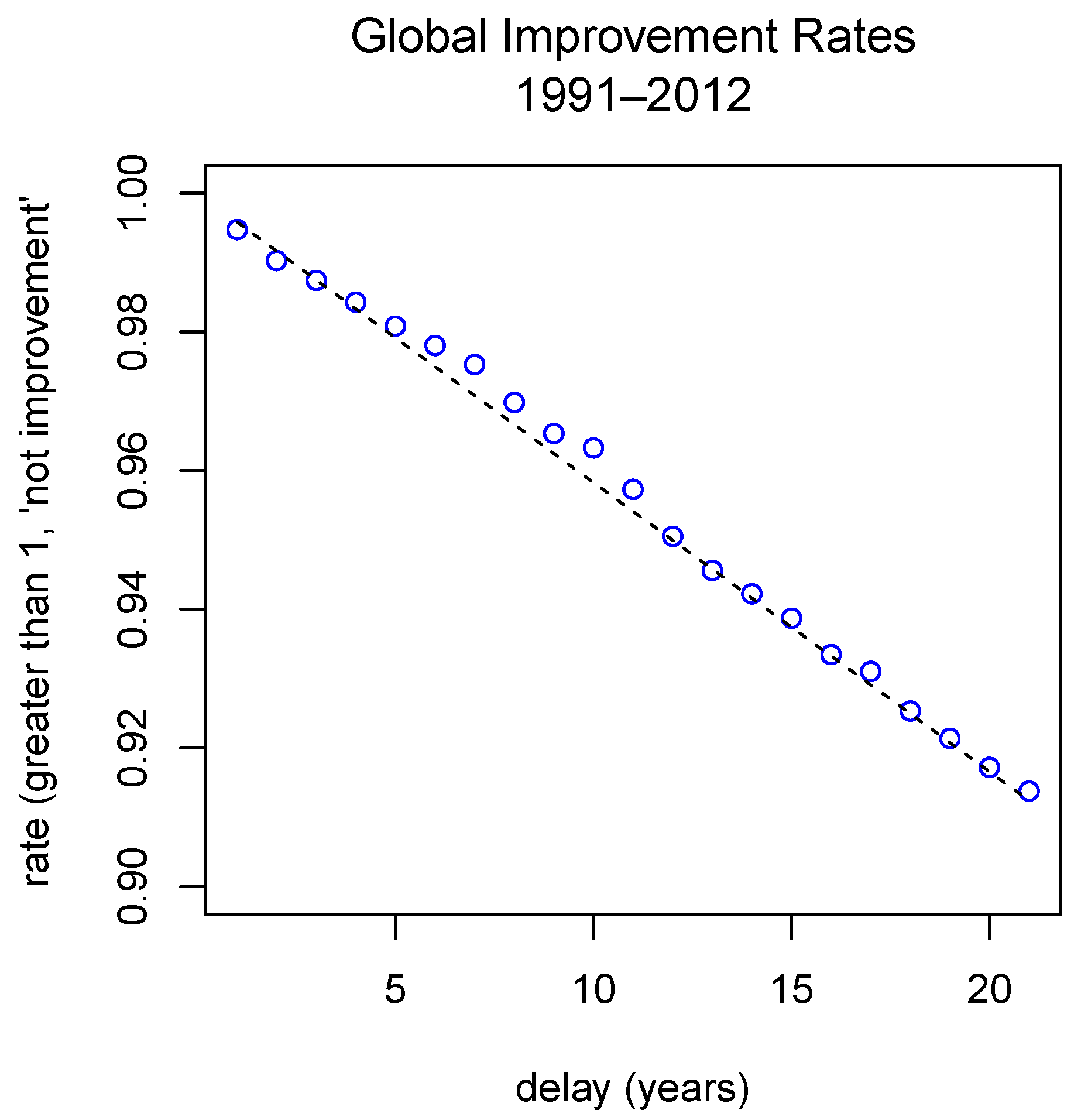
  • We estimate the mean, with respect to the delay, of the improvement rates:
    r ¯ ¯ d = 1 # ( d ) t 0 , t 1 : d = t 1 t 0 r ¯ t 0 t 1 ,
    being # ( d ) the number of couples ( t 0 , t 1 ) such that d =   t 1 t 0 . We will refer to these values as the global improvement rates for the delayd.
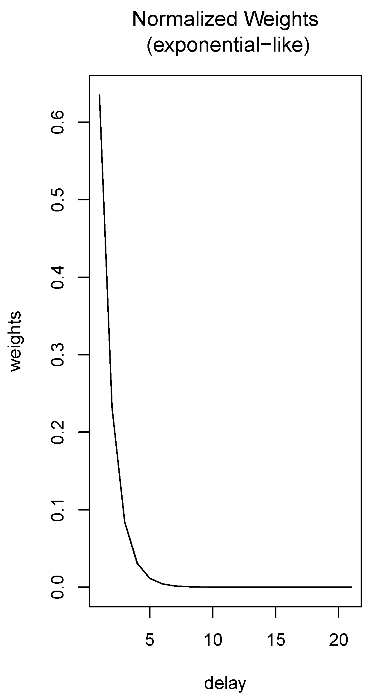
  • The annual improvement rates by delay, r ¯ ¯ d , play an important role in the procedure because they contain previous information of the mortality process. However, the experience of studying this phenomenon allows us to assure that the importance of these rates are not the same for all delays, and it is clear (under usual conditions such as non-pandemic ones) that the behavior of the improvement rates become more important if they are close to the time of prediction. Using this realistic assumption, we assume that the importance of these rates is modulated by a probability distribution function. In particular, we consider a modified exponential function. To do this, we consider the exponential probability density function with the form
    f λ s = λ e λ s if s 0 , 0 if s < 0 ,
    and obtain a density function in the interval [ 0 , h ] by putting
    f ^ λ s = λ e λ s 0 h λ e λ s d s , s [ 0 , h ] .
    Then, we define the density function ξ · from (6) by ξ s = f ^ λ s for s [ h , 0 ] .
    In the particular case when in the numerical approximations we consider only integer delays, we can discretize the interval [ 0 , h ] by using a finite number of integer delays s = 0 , 1 , , d max , where d max = h N is the maximum delay to be considered. Thus, instead of (17), we will use the discretized probability function
    f * s = f ^ λ s s = 0 d max f ^ λ s ,
    which approximates (17) at s = 0 , 1 , . . . , d max .
    Remark 3.
    We could also use the values of the function f ^ λ s at s = 0 , 1 , . . . , d max to define the approximative function f * s , but we have used (18) because the results in the numerical simulations were quite good. The use of the exponential function to derive f * is arbitrary. Thus, it is reasonable to think that the selected function is not optimal. In this sense, we consider that this topic could be a possible new line of investigation to improve the work.
  • Using the annual improvement rates, and the exponential distribution, we define the weighted improvement rates as
    R w e i g h t d = r ¯ ¯ d · f * d
  • Using the improvement rates by delay, r ¯ ¯ d , we can define the functions α s from (6), by putting
    α d = r ¯ ¯ d for d 0 , 1 , . . . , d max ,
    where r ¯ ¯ 0 = 1 , and then defininig α s at other points by linear interpolation, that is,
    α s = α i 1 + α i α i 1 ( s + i + 1 ) for s ( i 1 , i ) , i = 0 , . . . , d max 1 .
    This procedure can be implemented for a non-integer step as well. Namely, let b be a divisor of d max . Then, we define in a similar way as above the improvement rates r ¯ ¯ d for d = b , 2 b , . . . , d max . We observe that in this particular situation, the functions α s are independent of i D .
It is usual to assume some hypothesis in the behavior of the mortality. Namely,
H1.
For each age x, for an arbitrary moment t and for a small time step τ > 0 , the graduate value at t + τ , denoted by q x t + τ , depends on:
  • all graduate values at moment t, q z t , z D Z (via Gaussian kernel graduation, see [17]).
  • all previous moments of time t + s , s h , 0 (via the exponential probability density function and the improvement rates).
H2.
The relation between q x t + τ and q z t , q z t + s s h , 0 is:
q x t + τ = 1 1 + τ q x t + τ 1 + τ z D h 0 j x z q z t + s α s d μ s + τ 1 + τ z Z \ D h 0 j x z g z t + s α s d μ s
where j · is a suitable kernel (in this work a Gaussian kernel), g z · is the rate of death either at “negative ages” or after the actuarial infinite, d μ ( s ) = ξ s d s and α s is defined above using the annual improvement rates from the past.
Remark 4.
The hypothesis H2 is consistent in the sense that if τ 0 , then q x t + τ q x t . Additionally, if τ 0 , the new graduate value depends on the step τ and the delay.
Remark 5.
We note that if the history is not important, then the annual improvement rates are equal to 1, so μ s can be interpreted as a degenerated probability function such that d μ s = 1 at 0. In this situation, the expression (21) is analogous to (1).
Remark 6.
The proposed relation (21) is based on the empirical experience and on the actuarial practice in a similar way as in [10].
Next, we establish the relation between (21) and (6). From (21), we easily obtain that
1 + τ τ q x t + τ = q x t τ + z D h 0 j x z q z t + s α s d μ s + z Z \ D h 0 j x z g z t + s α s d μ s , q x t + τ q x t τ = z D h 0 j x z q z t + s α s d μ s q x t + τ + z Z \ D h 0 j x z g z t + s α s d μ s .
Formally, if we consider a fixed time t, and we take the limits as τ 0 , then
d d t q x t = z D h 0 j x z q z t + s α s d μ s q x t + z Z \ D h 0 j x z g z t + s α s d μ s .
Remark 7.
The validation of the model will be made using the observed values in the period 2013–2018 and the Lee-Carter model by taking the predicted values in both cases. This can be done showing that our predictions lie in the confidence interval of the predictions by the Lee-Carter model or even that they are near the expected value in this model.

3.1.2. Application of Theoretical Results

Equation (22) fits into model (6) with D = { 0 , . . . , 100 } , m = 101 and u i t = q i t . The Gaussian kernel obviosuly satisfies (H1) and (H2). The function g r t g ¯ r l 2 is a constant function, where g ¯ r is defined as follows:
g ¯ r = 0 if r < 0 , g 0 > 0 if r > 100 .
Hence, (H3) is satisfied. Here, g 0 is the probability of death after the actuarial infinite. In this case, α i s = α s , where α · C ( [ h , 0 ] , R ) is given in (20). Therefore, (H4) holds true. Since the function g does not depend on, the problem is autonomous, so we take τ = 0 .
Hence, Lemma 1 implies that for any initial condition ϕ C ( [ h , 0 ] , R m ) , there exists a unique solution u ·   C 1 ( [ 0 , + ) , R m ) , where we take τ = 0 . Additionally, in view of Proposition 1 if ϕ C h , 0 , R n is such that ϕ i s 0 for s h , 0 , i D , then u i t 0 for all i D , t 0 . This is an important property, because the functions q i t cannot be negative as they are probabilities.
We obtain that for small h there is a unique exponentially stable fixed point as well.
Lemma 7.
We choose h 0 > 0 such that
M 0 = h 0 0 α ( s ) d μ ( s ) 1 .
Then for any h h 0 such that
h < 1 2 log 1 δ 0 ,
where δ 0 = min r D { 1 M 0 i D j i r } , problem (22) possesses a unique fixed point which is exponentially stable.
Proof. 
Since j is a Gaussian kernel, i D j i r < 1 for any r, so M 0 1 implies that δ 0 > 0 . The result follows then from Remark 1 and Corollary 2. □
Although in the actuarial practice, the set D is finite because the probability of death is considered to be constant after some age (the actuarial infinite), it is also possible to estimate the values of q x for any non-negative x. In this case, D is of the type (5); more precisely, D = { i Z : i 0 } . As before, (H1), (H2), (H4) are satisfied and the function g r t g ¯ r is a constant function, where g ¯ r is defined by: g ¯ r = 0 if r < 0 .
If we consider the phase space X = l 1 , then g ¯ r l 2 , so (H3) is satisfied. As the Gaussian kernel j has subexponential growth, (H6) is true. Since α i s = α s for any i D , (H7) is obviously satisfied (which implies that (H5) also holds). Then, by Lemma 4 for any initial condition ϕ C ( [ h , 0 ] , l 1 ) there exists a unique solution u · C 1 ( [ 0 , + ) , l 1 ) . Additionally, in view of Proposition 2, if ϕ C h , 0 , l 1 is such that ϕ i s 0 for s h , 0 , i D , then u i t 0 for all i D , t 0 .
If we consider the phase space X = l 1 1 , then g ¯ r l 2 1 , so (H3b) is satisfied. Thus, Lemma 5 implies that for any initial condition ϕ C ( [ h , 0 ] , l 1 1 ) , there exists a unique solution u · C 1 ( [ 0 , + ) , l 1 1 ) . Finally, by Proposition 3 if ϕ C h , 0 , l 1 1 is such that ϕ i s 0 for s h , 0 , i D , then u i t 0 for all i D , t 0 .

3.2. Details and Example

In this section, we will give the details of the numerical simulations.

3.2.1. Data, Period and Software

The data used in this study are downloaded from the Human Mortality Data Base [18]. It refers to the death rates of the Spanish population in the period 1908–2018. In this study, we combine several sub-periods to obtain the estimations. The period 1908–2012 is used to obtain some preliminary estimates; a sub-period of them, 1978–2012, is used to fit the significant improvement rates. We note that this last sub-period coincides with a period of significant changes in Spain. Among other events, the actual democratic status begins, which motivates the consolidation of the welfare system and implies the consolidation or changes of health protocols in Spain such as the transfer of home births to the hospital, significantly reducing the mortality at first ages [41,42]. The period 2013–2018 is used to validate the method.
The software used for all calculations and the construction of the figures is the R-Software [43]. Additionally, the data are downloaded from [18] and they are manipulated and visualized using the R-package [44]. This demographic package is also used to estimate the Lee-Carter Model.

3.2.2. Validation

The validation process has two parts. In the first part, we compare the forecasted data with the observed data in the same period. In the second part, to validate the model, we compare the proposed method with the classical Lee-Carter model [28].
In the first part, we fit the proposed model using the observed data in the period 1978–2012; next, we forecast the mortality in the years 2013–2018 to obtain the prediction of the mortality rates, q x t , f . Then, for each year in the validation period, we compare the observed death rates at each age, q x t , o b s , with the forecasted values. The comparison is made using
I M S D t = x = 0 ω q x t , o b s q x t , f 2 q x t , f 2 or χ M S D t = x = 0 ω q x t , o b s q x t , f 2 q x t , f .
It is remarkable that a modification of the previous indicators can be appropriate. In particular, we can use the smoothed values and not the observed or forecasted values directly. We denote this modified indicators as I S M S D t and χ S M S D t .
The second part of the validation consists in comparing the proposed method in this work with the classical Lee-Carter model [28]. The comparison is made in two ways. Firstly, we forecast the mortality rates by the two methodologies in the period 2013–2018. Then, we compute I M S D t and χ M S D t (or its smoothed versions) and compare the results directly. Additionally, we project the mortality in the period 2019–2030 with both techniques and compare it to determine if they have a similar magnitude.
The Lee-Carter model was formulated to estimate the central mortality rates, m x t , at year t. This model can be formulated as
ln m x t = a x + k t b x + e x , t ,
where a x , b x are factors depending only on the age; k t is a factor that describes the evolution of the mortality over the years; e x t is a realization of the white noise. It is remarkable that b x modulates the factor k t to adequate the behavior of the mortality due to social improvements such as the control of diseases, the improvement in health habits, nutrition… If we consider this model without other conditions, the number of parameters is 2 × # ( n u m b e r o f a g e s ) + # ( n u m b e r o f y e a r s ) (in our case, 2 × 101 + 111 = 313 parameters). It is usual to model the k t values as an autoregressive process of type ARIMA, and also that the fit provides us an autoregressive model of order 1 (one parameter); in this case, we reduce the number of parameters to 202. It is convenient to remark that the Lee-Carter model is a parametric model and the proposed method is nonparametric. In this sense, the assumptions of the proposed model are less restrictive.
Remark 8.
The election of the Lee-Carter model is not arbitrary and it is justified by the importance of that work. The paper of Lee-Carter model [28] is considered as a seminal model. It is the model with more influence in all ambits of this field of knowledge. We note that, in the actuality, there exist several versions of this model that improve it. However, we consider the comparison with this model by several reasonings: (i) It is usual in the scientific literature to use this model in comparisons; (ii) others models based on the Lee-Carter model either are not better in all conditions or the improvements are small; (iii) the Lee-Carter model has a great number of parameters, 200 or more; comparing this fact with our model, the difference is significant, as the number is less in our case.

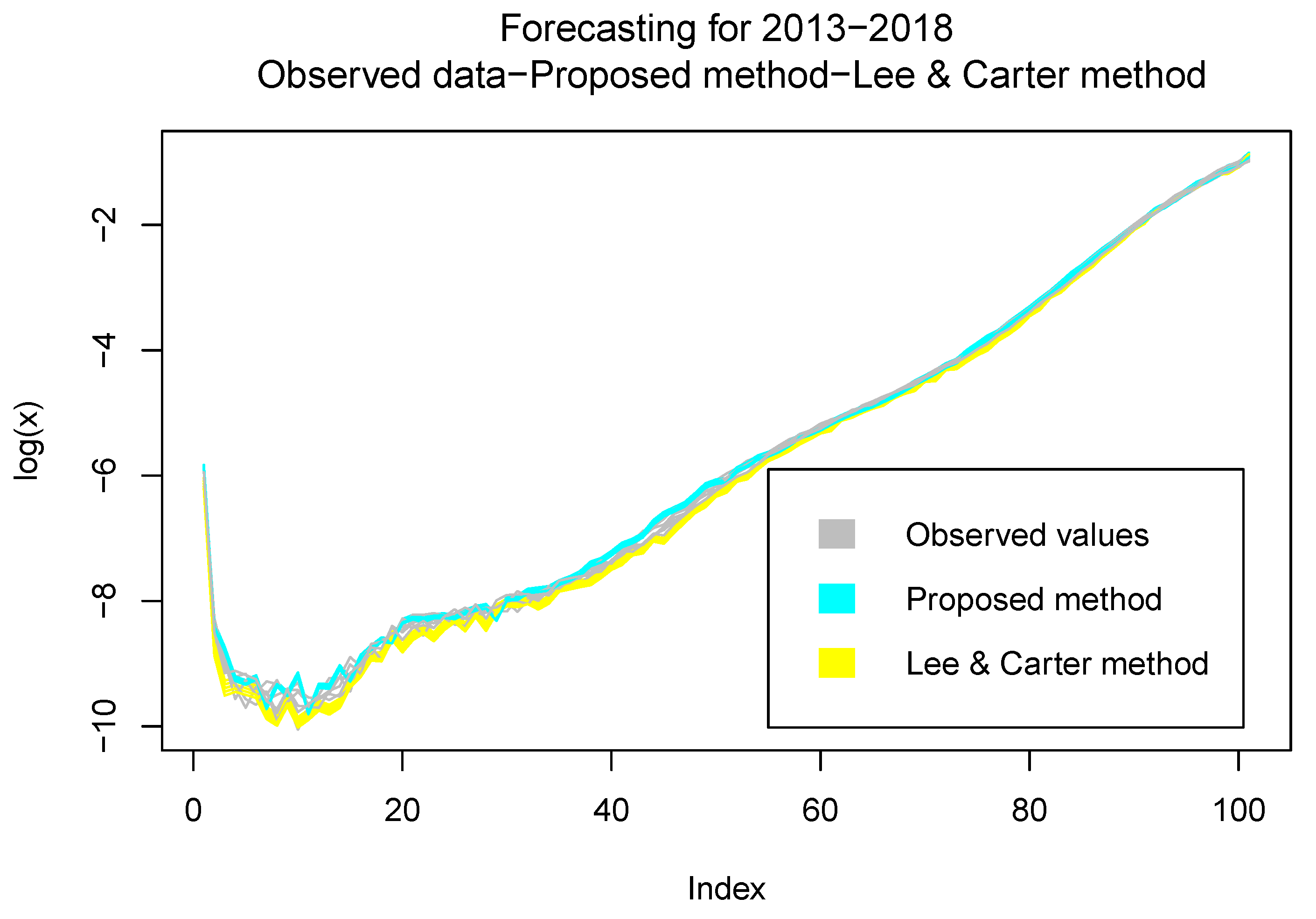
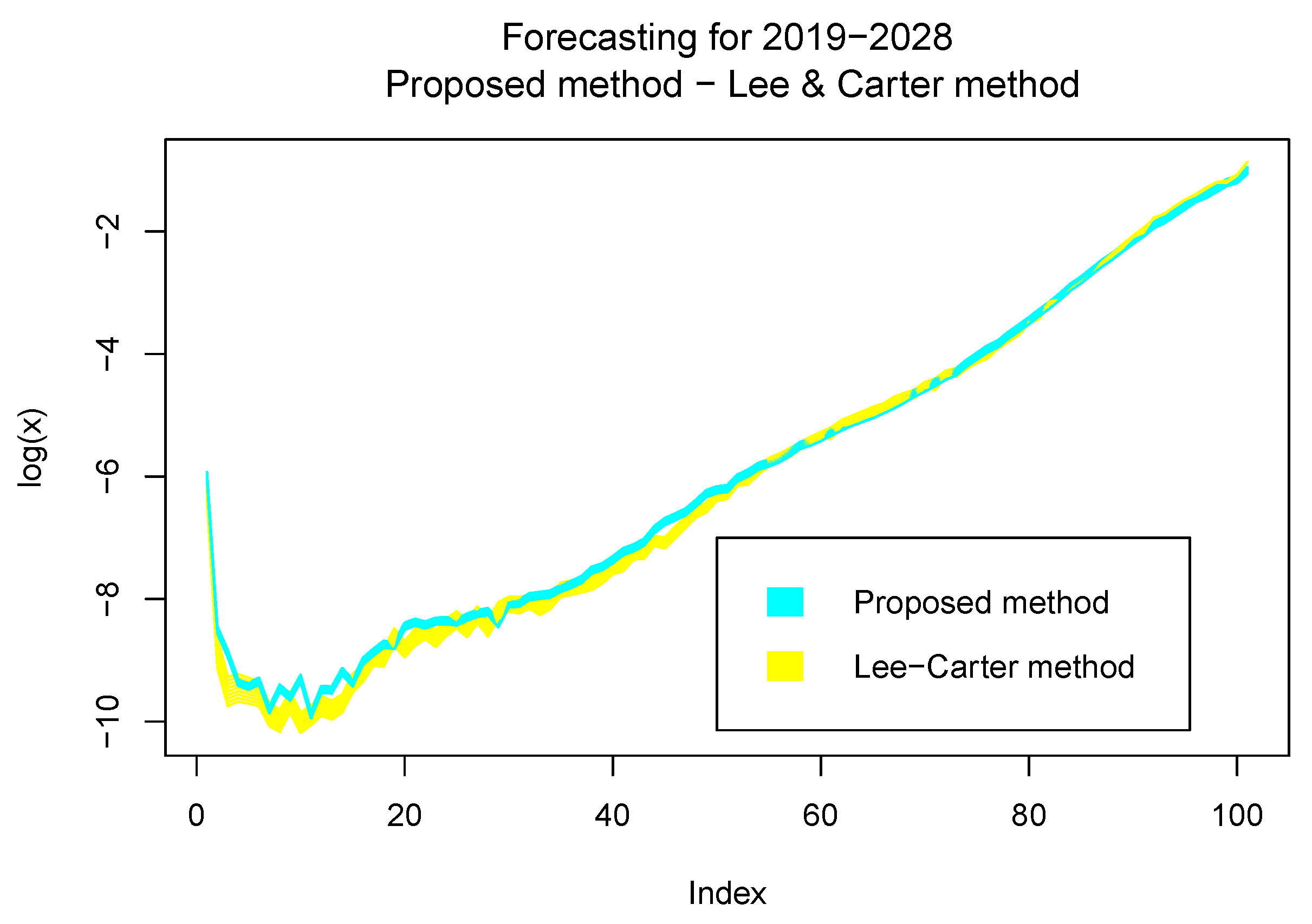
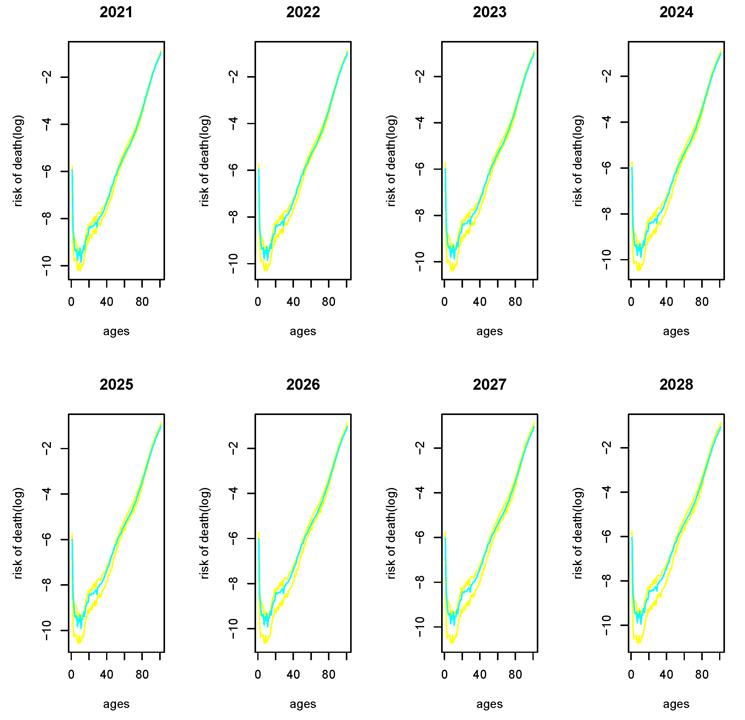
3.2.3. Estimations and Results

It is known that the mortality has a dynamic behavior in all country or regions. Figure 1 shows the evolution of the crude mortality rates in the period 1908–2018. This figure shows the evolution of the death rates over the last 111 years.
We note that the highest series in the graphic correspond to the first years of the study, at the beginning of the XX century. The lines at the bottom of the figure corresponds to the recent years. This indicates to us that there exists an evident improvement in the mortality rates.
In order to apply the expression (21) to the observed data and obtain the forecasted values, it is necessary to know the values of the function g z after the actuarial infinite. In this work, we consider that these values correspond to the values of the mortality rates for ages greater than a characteristic age, when an effect known as “Plateau effect” begins [45,46]. This effect indicates to us that the risk of death does not increase to 1, but remains constant from certain age. Figure 1 shows this effect (simulated to facilitate interpretation), which can be observed in the final part of each curve and corresponds to the mortality risk values for ages in the range 90–130. In practice, the age at which the Plateau effect begins is unknown and it can be only estimated from the observed data. In this work, we consider that, for each year t greater than a characteristic age, g z t = max q z t z > 70 . Figure 2 shows the evolution of the death risk at last ages.
The tendency of the series in Figure 2 is decreasing and the values of this series converge to the limit 0.35 (blue line at the bottom of the figure), which is consistent with the works of other authors ([40], p. 41) in the Spanish case, for both genders and for ages up to 105 years. Other authors consider that this limit is 0.684 [46] (yellow-middle line in the figure), or 0.5 [45] (pink-top line in the figure). This type of assertion is not without controversy [47]. In our simulations, we have taken g z 2012 0.385638 as the probability of death after the actuarial infinite. This is the value of g 0 in (23).
In step 2 of the method, the global improvement rates are estimated using (16). Figure 3 shows these rates for the first 21 lags; we find that the behavior is similar to the first 40 lags. We have analyzed these first delays and consider that they are enough to capture the dynamic of the improvements. Due to this, we have chosen the value of h equal to 21 .
We fit a linear model for the global improvement rates (dashed line in Figure 3) without the constant coefficient and the obtained value of the parameter is b ^ = 0.004171019 . In this method, we consider as global improvement rates the values derived from the expression r ¯ ¯ d = r ¯ ¯ d = 1 + b ^ · d , d 1 , 2 , , 21 . Hence, with such a procedure, the function α s is linear.
On other hand, we assume that the impact of the improvement rates is not equal for all of them. Its importance is modulated by another function. As we have said, the improvement rates are modulated by a probability function which is exponential, as in expression (18), and the weigthed improvement rates are obtained as in (19). The parameter λ in (18) is equal to 11 12 . Figure 4 shows the probability function which is used.
Now, we have defined all the elements which are necessary to apply the method for forecasting.
In order to estimate the solution, we use expression (21) with τ = 1 and approximate the integral term with the Riemann summatory.
Firstly, and with the objective of using the observed data to measure the quality of the technique, we apply the method using the data in the period 1908–2012 and obtain two types of predictions for the period 2013–2018: (i) applying the proposed technique; (ii) applying the Lee-Carter method. Additionally, the indicators of quality defined by (24) are estimated.
Figure 5 shows the predictions with the two techniques, the proposed technique and the Lee-Carter method. We can observe that these two series of values are close to the observed data. The magnitude of the values are coherent in the two methods. Comparing them with a graphical analysis, we are not able to identify whether one method is better than the other.
In order to clarify if one technique is better than the other, we need to calculate a numerical indicator. In this sense, we consider the quality indicators defined in (24). Using the observed data as reference data and the estimation made with each technique as the assumption, we obtain the values in Table 1.
We can observe that the proposed technique is more accurate that the Lee-Carter method in both indicators of goodness. In the case of the indicators I M S D t , the improvement is for all years and the values of the error of the proposed technique with respect to the observed values are between 30 % and 80 % of the error of the Lee-Carter model. In the case of the indicators χ M S D t , we observe that the improvement is not for all years, as in 2015, the Lee-Carter model has better results, but we think that this occurs because that year has a great oscillation at initial ages. For the rest of the years, the rate of improvement of the proposed method with respect to the Lee-Carter model was between 30 % and 80 % .
Now, as we said before, we will compare the proposed technique with the Lee-Carter method in forecasting. Figure 6 shows the predictions with these two methods for the period 2019–2028.
We observe that the Lee-Carter method has greater variability than the proposed method for the ages in the intervals 5–15 and 40–50. In addition, the mortality curves have similar values for the rest of the ages. As we do not have observed values of mortality for the period 2019–2028, it is difficult to determine which of the two techniques is better. In this situation, we will only compare the magnitude of the predictions with these two techniques, checking whether the values are similar or not. Since the Lee-Carter method is a reference method, we will verify if our results are within the confidence intervals of the Lee-Carter predictions. Figure 7 shows the values of the predictions with the proposed technique jointly with the upper and lower confidence curves of the Lee-Carter predictions (at a 95% confidence-level) for the years 2021–2028. It is clear that the values are between the two bounds of the Lee-Carter model, which indicates us that the method is appropriate. Additionally, considering that with the predictions between 2013 and 2018, the proposed method has turned out to be more accurate than the Lee-Carter method, it is convenient to reflect on which of these methods is appropriate.
We note that we can measure the goodness of the forecasting otherwise by using the quality indicators (24) but changing the reference values. First, we must assume as correct the values of the Lee-Carter values; second, we assume as correct the values of the proposed method. The comparison is made using the caution principle, depending of the application. For example, if we use the values of the proposed method when the true values are the Lee-Carter ones, the indicator I M S D 2019 was equal to 1.812869 , which tells us that “globally” the discrepancies were close to 81 % . If we use the Lee-Carter values when the true values are the ones of the proposed technique, then I M S D 2019 was 2.551214 , which indicates to us that, “globally”, discrepancies were close to 155 % . The “possible error” was double if we used the Lee-Carter values. The same situation occurs for the rest of the years.
These two ways of measuring the quality of the proposed method allow us to affirm that, in the middle-term, the proposed method is quite appropriate.
It is important to point out that there exist several ways to improve this work: (i) introducing one improvement rate for each age instead of estimating a unique improvement rate for all ages, q · t 1 = r ¯ t 0 , t 1 · q · t 0 (obviously, this increases the number of parameters of the problem, but no more than in the Lee-Carter model); (ii) introducing a process that allows us to select the better probability function.
Finally, we would like to remark that the main differences in the numerical simulations of this paper with respect to the ones in [10] are the following:
  • In the model of this paper, we have considered the influence of the values of the variable in the past and not only in the current moment of time, as in [10].
  • The functions α s are new in this paper and we have approximated them via the improvement rates r ¯ ¯ d .
  • We have considered the probability functions (17), (18) in order to modulate the improvement rates r ¯ ¯ d .
  • In [10], the value of the function g was taken to be equal to 0 outside the domain D, whereas in the present work, the value of g for ages greater than 100 was taken to be equal to a positive number due to the “Plateau effect”.
  • The numerical simulations show that the predictions are good enough for at least a period of 8 years, whereas in the model without delay, the predictions were good for a period of 3 years.

4. Conclusions

In this work, we considered a system of ordinary differential equations with non-local discrete diffusion and finite delay. This paper extends the results in [10], incorporating prior information in the form of delay. With this, it is possible to improve the prediction window with respect to the previous work; in [10], the horizon of the prediction is adequate up to three years; however, in this work, it is verified (with the data in the considered period and for the defined measures) that the prediction horizon can be extended up to 8 years, and that it gives coherent values, in magnitude, when we compare it with other classical techniques such as the Lee-Carter model, up to 18 years.
The first part of the paper is dedicated to theoretically analyzing the system: firstly, a system with a finite number of equations; secondly, a system with an infinite number of them. In both cases, we prove the existence of solutions and several properties of them such as comparison results, stability and symmetry.
In the second part of the work, we applied the model to life tables, defining the parameters of the model (for example, the delay is incorporated as improvement rates of the probability of death) and applying the theoretical results of the first part by estimating and projecting to the future the risk of mortality (by age). In order to calculate the numerical estimations, we considered the data of Spanish mortality in the period 1908–2018 from [18]; the choice of this source of information is due to the fact that this organization uses a methodology that unifies certain methodological aspects of the statistical bureaus of several countries, providing a common framework that allows us to assure that the proposed model can be applied to any region in the world. In order to validate the proposed model and compare it with the Lee-Carter model, we defined some indicators of goodness and smoothness. In this sense, these measures indicate to us that this model is more accurate than the classical Lee-Carter model in the considered period of validation (between 2013 and 2018). Additionally, the proposed model gives us coherent values up to 2028 (maybe even for a larger period of time) when we compare these values with the values of the Lee-Carter model.
Finally, we consider several aspects of this work that could be improved in future researches. For example, we could consider improvement rates which are dependent of age or use other density probability functions, and not only the exponential distribution. It is possible to introduce other aspects in the model as the cohort effect, which is usual in the demographic and actuarial fields.

Author Contributions

Conceptualization, F.M. and J.V.; methodology, F.M. and J.V.; software, F.M. and J.V.; validation, F.M. and J.V.; formal analysis, F.M. and J.V.; investigation: F.M. and J.V.; resources, F.M. and J.V.; writing—original draft preparation, F.M. and J.V.; writing—review and editing, F.M. and J.V.; visualization, F.M. and J.V.; supervision, F.M. and J.V.; project administration, F.M. and J.V.; funding acquisition, F.M. and J.V. All authors have read and agreed to the published version of the manuscript.

Funding

This research was funded by the projects PGC2018-096540-B-I00 (Spanish Ministry of Science, Innovation and Universities), PID2019-108654GB-I00 (Spanish Ministry of Science and Innovation), P18-FR-4509 and P18-FR-2025 (Junta de Andalucía).

Institutional Review Board Statement

Not applicable.

Informed Consent Statement

Not applicable.

Data Availability Statement

The data that support the findings of this study are openly available in Human Mortality Data Base at www.mortality.org or www.humanmortality.de.

Acknowledgments

We woud like to express our gratitude to the reviewers for their useful comments and remarks.

Conflicts of Interest

The authors declare no conflict of interest.

References

  1. Fife, P. Some nonclassical trends in parabolic and parabolic-like evolutions. In Trends in Nonlinear Analysis; Springer: Berlin, Germany, 2003; pp. 153–191. [Google Scholar]
  2. Cortazar, C.; Elgueta, M.; Rossi, J.D. Nonlocal diffusion problems that approximate the heat equations with Dirichlet boundary conditions. Israel J. Math. 2009, 170, 53–60. [Google Scholar] [CrossRef]
  3. Pérez-Llanos, M.; Rossi, J.D. Numerical approximations for a nonlocal evolution equations. SIAM J. Numer. Anal. 2012, 49, 2103–2123. [Google Scholar] [CrossRef] [Green Version]
  4. Bates, P.; Fife, P.; Ren, X.; Wang, X. Travelling waves in a convolution model for phase transitions. Arch. Ration. Mech. Anal. 1997, 138, 105–136. [Google Scholar] [CrossRef]
  5. Bates, P.; Chmaj, A. A discrete convolution model for phase transitions. Arch. Ration. Mech. Anal. 1999, 150, 281–305. [Google Scholar] [CrossRef]
  6. Bates, P.; Chmaj, A. An integrodifferential model for phase transitions: Stationary solutions in higher dimensions. J. Stat. Phys. 1999, 95, 1119–1139. [Google Scholar] [CrossRef]
  7. Bates, P.; Han, J. The Dirichlet boundary problem for a nonlocal Cahn-Hilliard equation. J. Math. Anal. Appl. 2005, 311, 289–312. [Google Scholar] [CrossRef]
  8. Chasseigne, E.; Chaves, M.; Rossi, J.D. Asymptotic behavior for nonlocal diffusion equations. J. Math. Pures Appl. 2006, 86, 271–291. [Google Scholar] [CrossRef] [Green Version]
  9. Bogoya, M.; Gómez S., C.A. Discrete model of a nonlocal diffusion equation. Rev. Colomb. Mat. 2013, 47, 83–94. [Google Scholar]
  10. Morillas, F.G.; Valero, J. On a nonlocal discrete diffusion system modeling life tables. Rev. R. Acad. Cienc. Exactas Fis. Nat. Ser. A Mat. RACSAM 2014, 108, 935–955. [Google Scholar] [CrossRef]
  11. Cairns, A.J.G.; Blake, D.; Dowd, K. Modelling and management of mortality risk: A review. Scand. Actuar. J. 2008, 2008, 79–113. [Google Scholar] [CrossRef]
  12. Hale, J.K. Theory of Functional Differential Equations; Springer: New York, NY, USA, 1977. [Google Scholar]
  13. Amigó, J.M.; Giménez, A.; Morillas, F.; Valero, J. Attractors for a lattice dynamical system generated by non-newtonian fluids modelling suspensions. Internat. J. Bifur. Chaos 2010, 20, 2681–2700. [Google Scholar] [CrossRef]
  14. European Parliament and of the Council. Risk Management and Supervision of Insurance Companies (Solvency II)-Consolidated text: Directive 2009/138/EC of the European Parliament and of the Council of 25 November 2009 on the Taking-Up and Pursuit of the Business of Insurance and Reinsurance. Available online: https://eur-lex.europa.eu/ (accessed on 6 December 2020).
  15. Chiang, C.L. The Life Tables and Its Applications; Krieger Publishing Company: Malabar, FL, USA, 1984. [Google Scholar]
  16. Benjamin, B.; Pollard, J.H. The Analysis of Mortality and Other Actuarial Statistics; Institute of Actuaries and the Faculty of Actuaries: Oxford, UK, 1993. [Google Scholar]
  17. Ayuso, M.; Corrales, H.; Guillén, M.; Perez-Marín, A.M.; Rojo, J.L. Estadística Actuarial Vida; Universitat de Barcelona, Edicions: Barcelona, Spain, 2007. [Google Scholar]
  18. University of California, Berkeley (USA); Max Planck Institute for Demographic Research (Germany). Human Mortality Database. Series of Death Rates of Spain. Available online: www.mortality.org (accessed on 1 December 2020).
  19. Instituto Nacional de Estadística (Statistics National Institute of Spain). Life Tables: Methodolgy. Available online: https://ine.es/en/metodologia/t20/t2020319a_en.pdf (accessed on 6 December 2020).
  20. Gompertz, B. On the nature of the function of the law of human mortality and on a new mode of determining the value of life contingencies. Trans. R. Soc. 1825, 115, 513–585. [Google Scholar]
  21. London, D. Graduation: The Revision of Estimates; ACTEX Publications: New Hartford, CT, USA, 1985. [Google Scholar]
  22. Beer, J. Dealing with uncertainty in population forecasting (Statistics Netherlands). Available online: https://www.cbs.nl/-/media/imported/documents/2000/24/dealing-with-uncertainty.pdf (accessed on 21 December 2020).
  23. Helligman, L.M.A.; Pollard, J.H. The age pattern of mortality. J. Inst. Actuar. 1980, 107, 49–82. [Google Scholar] [CrossRef]
  24. Forfar, D.O.; McCutcheon, M.A.; Wilkie, M.A. On graduation by mathematical formula. J. Inst. Actuar. 1988, 115, 1–149. [Google Scholar] [CrossRef]
  25. Gavin, J.; Haberman, S.; Verrall, R. Moving weighted average graduation using kernel estimation. Insur. Math. Econ. 1993, 12, 113–126. [Google Scholar] [CrossRef]
  26. Debón, A.; Montes, F.; Sala, R. A comparison of parametric models for mortality graduation. Application to mortality data for the Valencia Region (Spain). SORT Stat. Oper. Res. 2005, 29, 269–288. [Google Scholar]
  27. Villegas, A.M.; Kaishev, V.K.; Millossovich, P. StMoMo: A R package for stochastic mortality modeling. J. Stat. Softw. 2018, 84, 1–38. [Google Scholar] [CrossRef] [Green Version]
  28. Lee, R.; Carter, L. Modelling and forecasting US mortality. J. Am. Stat. Assoc. 1992, 87, 659–671. [Google Scholar]
  29. Debón, A.; Montes, F.; Sala, R. A comparison of models for dynamic life tables. Application to mortality data from the Valencia Region (Spain). Lifetime Data Anal. 2006, 12, 223–244. [Google Scholar] [CrossRef]
  30. Debón, A.; Montes, F.; Puig, F. Modelling and forecasting mortality in Spain. Eur. J. Oper. Res. 2008, 189, 624–637. [Google Scholar] [CrossRef] [Green Version]
  31. Haberman, S.; Renshaw, A. On age-period-cohort parametric mortality rate projections. Insur. Math. Econ. 2009, 45, 255–270. [Google Scholar] [CrossRef] [Green Version]
  32. Dodd, E.; Forster, J.J.; Bijak, J.; Smith, P.W.F. Smoothing mortality data: Producing the English life table, 2010–2012. J. R. Stat. Soc. Ser. A Stat. Soc. 2016, 181, 1–19. [Google Scholar] [CrossRef] [Green Version]
  33. Copas, J.B.; Haberman, S. Non-parametric graduation using kernel methods. J. Inst. Actuar. 1983, 110, 135–156. [Google Scholar] [CrossRef]
  34. Morillas, F.G.; Baeza, I.; Pavia, J.M. Risk of death: A two-step method using wavelets and piecewise harmonic interpolation. Estadística Española 2016, 58, 245–264. [Google Scholar]
  35. Morillas, F.G.; Sampere, I.B. Using wavelet techniques to approximate the subjacent risk of death. In Modern Mathematics and Mechanics; Sadovnichiy, V.A., Zgurovsky, M.Z., Eds.; Springer International Publishing: Cham, Switzerland, 2019; Chapter 28; pp. 541–557. [Google Scholar]
  36. Brouhns, N.; Denuit, M.; Keilegom, I.V. Bootstrapping the Poisson log-bilinear model for mortality forecasting. Scand. Actuar. J. 2005, 2005, 212–224. [Google Scholar] [CrossRef]
  37. Dodd, E.; Forster, J.J.; Bijak, J.; Smith, P.W.F. Stochastic modelling and projection of mortality improvements using a hybrid parametric/semi-parametric age–period–cohort model. Scand. J. 2020. [Google Scholar] [CrossRef]
  38. Haberman, S.; Renshaw, A. Parametric mortality improvement rate modelling and projecting. Insur. Math. Econ. 2012, 50, 309–333. [Google Scholar] [CrossRef]
  39. Haberman, S.; Renshaw, A. Modelling and projecting mortality improvement rates using a cohort perspective. Insur. Math. Econ. 2013, 53, 150–168. [Google Scholar] [CrossRef] [Green Version]
  40. Albarrán Lozano, I.; Ariza Rodríguez, F.; Cóbreces Juárez, V.M.; Durbán Reguera, M.L.; Rodríguez-Pardo del Castillo, J.M. Riesgo de Longevidad y su aplicación práctica a Solvencia II. VIII International Awards “Julio Castelo Matrán”, Fundación Mapfre. Available online: https://www.fundacionmapfre.org/fundacion/es_es/publicaciones/diccionario-mapfre-seguros/r/riesgo-de-longevidad.jsp (accessed on 21 December 2020).
  41. Montes, M.J. Las Culturas del Nacimiento. Ph.D. Thesis, Universitat Rovira i Virgili, Tarragona, Spain, 2007. [Google Scholar]
  42. Lledó, J.; Pavía, J.M.; Morillas, F.G. Transformaciones en la distribución semanal de nacimientos. Un análisis temporal 1940–2010. Revista Española Investigaciones Sociológicas 2017, 159, 151–162. [Google Scholar] [CrossRef]
  43. R Core Team. R: A Language and Environment for Statistical Computing; R Foundation for Statistical Computing: Vienna, Austria, 2020; Available online: https://www.R-project.org/ (accessed on 21 December 2020).
  44. Hyndman, R.J. (with Contributions from Heather Booth, Leonie Tickle and John Maindonald). Package Demography: Forecasting Mortality, Fertility, Migration and Population Data (R Package Version 1.22). 2019. Available online: https://CRAN.R-project.org/package=demography (accessed on 21 December 2020).
  45. Dolgin, E. Longevity data hint at no natural limit on lifespan. Nature 2018, 559, 14–15. [Google Scholar] [CrossRef]
  46. Barbi, E.; Lagona, F.; Marsili, M.; Vaupel, J.W.; Kenneth, W.W. The plateau of human mortality: Demography of longevity pioneers. Science 2018, 360, 1459–1461. [Google Scholar] [CrossRef] [PubMed] [Green Version]
  47. Dong, X.; Milholland, B.; Vijg, J. Evidence for a limit to human lifespan. Nature 2016, 538, 257–259. [Google Scholar] [CrossRef] [PubMed]
Figure 1. Rates of death.
Mathematics 09 00220 g001
Figure 2. Last mortality rates.
Mathematics 09 00220 g002
Figure 3. Improvement rates.
Mathematics 09 00220 g003
Figure 4. Normalized weights.
Mathematics 09 00220 g004
Figure 5. Forecasting.
Mathematics 09 00220 g005
Figure 6. Long-term forecasting.
Mathematics 09 00220 g006
Figure 7. Comparison by using the confidence intervals of the Lee-Carter method.
Mathematics 09 00220 g007
Table 1. Summary of the measures of goodness of the predictions.
I M S D 2013 I M S D 2014 I M S D 2015 I M S D 2016 I M S D 2017 I M S D 2018
Model 0.05461045 0.06223897 0.02171756 0.03676833 0.02777047 0.03182172
Lee-Carter 0.08731890 0.11195858 0.02715306 0.09994482 0.07357846 0.10755673
%Improve. 62.5 55.6 80.0 36.8 37.7 29.6
χ M S D 2013 χ M S D 2014 χ M S D 2015 χ M S D 2016 χ M S D 2017 χ M S D 2018
Model 0.1641217 0.2378390 0.1283401 0.2026115 0.1892803 0.2083615
Lee-Carter 0.1919128 0.2775853 0.0947843 0.2470046 0.2353773 0.3415634
%Improve. 85.5 85.7 135.4 82.0 80.4 61.0
Publisher’s Note: MDPI stays neutral with regard to jurisdictional claims in published maps and institutional affiliations.

