A New Synchronization Method for Time-Delay Fractional Complex Chaotic System and Its Application

Abstract

This paper proposes a class of time-delay fractional complex $L\ddot{u}$ system and utilizes the adomian decomposition algorithm to study the dynamics of the system. Firstly, the time chaotic attractor, coexistence attractor and parameter space are studied. The bifurcation diagram and complexity are used to analyze the dynamic characteristics of the system. Secondly, the definition of modified fractional projective difference function synchronization (MFPDFS) is introduced. The corresponding synchronous controller is designed to realize the MFPDFS of the time-delay fractional complex $L\ddot{u}$ system. Thirdly, based on the background of wireless speech communication system (WSCs), the MFPDFS controller is used to realize the secure speech transmission. Finally, the effectiveness of the controller is verified by numerical simulation. The signal-noise ratio (SNR) analysis of speech transmission is given. The performance of secure communication is verified by numerical simulation.

1. Introduction

Works on fractional calculus have grown steadily and are now in full swing with applications to complex chaotic systems that appeared in [1,2,3,4,5]. Based on the experience gained in the study of integer complex chaos synchronization, many scholars then applied several methods for synchronization of fractional complex chaotic systems using feedback control, active control, sliding control, fuzzy control, and other methods. Zheng [6] introduced a fuzzy prediction based on feedback control methodology to stabilize the fractional order R$\ddot{o}$ssler system on its equilibrium. Li et al. [7] proposed a communication scheme for signal encryption and decryption, and designed an adaptive sliding mode controller to realize the synchronization stage between the encryption systems. Jiang et al. [8] discussed the sliding mode control of a class of fractional chaotic systems with variable order, and the stability of the designed controller are analyzed in detail. Wu et al. [9] discussed the finite time inter layer projection synchronization of a class of fractional order two-layer networks, set the synovial controller, and studied the finite time inter layer synchronization and finite time inter layer anti synchronization of fractional order two-layer networks. Chan et al. [10] proposed a secure communication scheme, which can resist the interference affecting the transmitter and transmission process by using the sliding mode observer. Khettab et al. [11] proposed an improved fuzzy adaptive control strategy for a class of nonlinear fractional order chaotic systems. The fractional order chaotic system is identified, and the stability of the proposed control method is analyzed. Physical real-world systems are often in fractional form and therefore they are more sensible to use fractional calculus instead of integer calculus to study physical phenomena. With the continued quest to advance the understanding of nonlinear dynamics and chaos, a wide range of approaches are employed including the construction of time-delay chaotic systems. Fractional order chaotic system has been successfully applied in chaotic secure communication, image encryption, fuzzy neural network analysis, and multimedia encryption technology. Pisarchik et al. [12] proposed a safety communication system with extreme multi-static electricity, when complete synchronization is achieved, information will be transmitted in a relatively short time. Bendoukha et al. [13] studied the dynamics of a fractional order chaotic system, which corresponds to the original Chua’s system with the same nonlinearity, and designed a secure communication scheme based on chaotic keying modulation. Liu et al. [14] proposed the definition of fractional difference function synchronization and completed the transmission simulation of an analog signal, digital signal, speech signal, and image signal. Zhang et al. [15] proposed a new color image encryption algorithm and used a hybrid model of bidirectional circular arrangement and DNA masking. Lai et al. [16] designed a controller to switch between two chaotic attractors. On this basis, a chaotic image encryption algorithm is proposed. The performance of the algorithm is numerically analyzed. Wang et al. [17] constructed a T-S fuzzy neural network model as a general approximator to approximate these uncertainties and unknown parameters, and established an adaptive sliding mode control scheme. Bhatnagar et al. [18] proposed biometric-inspired multimedia encryption technology to complete the encryption of multimedia data, and used a reliable decryption process to construct the original multimedia data from the encrypted data. Cai et al. [19] proposed a high data rate discontinuous chaotic communication scheme, which can meet the demand of explosive growth in data traffic and the design of multi-mode signal ensures that all sub carriers and time periods are fully utilized to transmit information bits.

In 2013, Luo analyzed the dynamic characteristics of the fractional-order complex Lorenz system and the fractional-order complex Chen system [20,21], studied their synchronization methods, and designed digital communication schemes to improve the performance of secure communication. In the same year, Liu proposed a fractional-order complex T system [22]. From the symmetry of the system, the stability of the equilibrium point, the bifurcation and the differential order when the system parameters change, the chaotic characteristics of the system were studied, and the feedback control technology was used to design the controller to give the analysis of the function projective synchronization scheme of the fractional complex T system. In 2014, Jiang proposed a fractional-order complex $L\ddot{u}$ system and studied its chaotic characteristics including the symmetry of the system, the stability of the equilibrium point and the bifurcation of the differential order. They used the method of active control and state observer to realize its anti-synchronization [23].

An application of chaotic encryption of particular interest here is in wireless speech communication [19]. A well designed encryption scheme prevents unauthorized parties from eavesdropping while also improving the disturbance rejection and fidelity. Based on the characteristics of WSCs, the time-delay fractional complex $L\ddot{u}$ communication system is realized by using the broadband characteristics and sensitivity to the initial value of the chaotic system. The design of the system is simple, flexible, and the security provided is better than the traditional chaotic masking encryption.

The main contributions of this paper are as follows:

(1)

The adomian decomposition algorithm is used to research the time-delay fractional complex $L\ddot{u}$ system. According to the complexity algorithm and bifurcation diagram, the chaotic characteristics are analyzed from two aspects: Parameters and fractional-order.

(2)

The definition of MFPDFS for the time-delay fractional complex $L\ddot{u}$ system is proposed, and feedback control is added to design the controller to realize the MFPDFS.

(3)

According to the designed MFPDFS controller, a WSCs secure communication scheme is designed. The signal at the receiver consists of the sum of the information signal and the time-delay fractional complex chaotic signal.

The rest of this paper is structured as follows: In Section 2, dynamics characteristics of the time-delay fractional complex $L\ddot{u}$ system are studied. In Section 3, the definition of MFPDFS for time-delay fractional complex $L\ddot{u}$ systems is given, a MFPDFS synchronous controller is designed, and the mathematical proof is provided. In Section 4, a block diagram of a WSCs is designed to encrypt the transmission of speech signals. In Section 5, simulations are performed to evaluate the effectiveness of the MFPDFS controller and implement speech transmission encryption. Finally, the study is summarized in Section 6.

2. Dynamics Characteristics of the Time-Delay Fractional Complex $\mathit{L}\ddot{\mathit{u}}$ System

The mathematical background of fractional range definition is as follows.

Definition 1.

In this paper, we use the Caputo definition as it includes the conventional initial conditions and Caputo derivative of the constant is zero (see [24]).

$$D_t^{q}f\left(t\right)=\frac{1}{\Gamma (m-q)}{\int }_0^t\frac{f\left(m\right)\left(\tau \right)d\tau }{(t-\tau )(q+1-m)}$$

(1)

where $m-1<q<m$, m is the first integer greater than q,$\Gamma (\ast )$ is the gamma function. The gamma function is expressed:

$$\Gamma \left(\alpha \right)={\int }_0^{\infty }{e}^{-t}{t}^{\alpha -1}dt.$$

(2)

Definition 2.

The adomian decomposition algorithm is a time-domain approximation algorithm that is more suitable for solving fractional-order systems. It can not require discretization and a large amount of memory to provide high-precision, fast-convergent approximate numerical solutions. For the fractional chaotic system $x\left(t\right)=f\left(x\right(t\left)\right)+g\left(t\right)$, where $x\left(t\right)=[x_1\left(t\right),\cdots ,x_n\left(t\right)]$, it is a given function variable, and $g\left(t\right)$ is a constant. The specific adomian algorithm expression is (see [25]):

$$\begin{array}{c}\hfill \begin{array}{c}\left\{\begin{array}{ccc}{D}_t^{q}x\left(t\right)\hfill & =\hfill & Lx\left(t\right)+Nx\left(t\right)+g\left(t\right)\hfill \\ x\left(k\right)t^{+}\hfill & =\hfill & b_k,k=0,\cdots ,m-1\hfill \\ x\left(k\right)t^{+}\hfill & =\hfill & b_k,k=0,\cdots ,m-1\hfill \end{array}\right.\hfill \end{array}\end{array}$$

(3)

where $D_t^q$ is the order of the q Caputo operator, L is the linear part of the system, N is the nonlinear part of the system, and $b_k$ is the initial value.

In this paper, the time-delay characteristic is introduced into the existing complex $L\ddot{u}$ system, the time-delay fractional complex $L\ddot{u}$ system is proposed, and its chaotic characteristics is analyzed in terms of time-delay, coexistence attractor, parameter space, complexity, and bifurcation diagram. The equations of a time-delay fractional complex $L\ddot{u}$ system are as follows:

$$\begin{array}{c}\hfill \begin{array}{c}\left\{\begin{array}{ccc}{D}_{*}^{q_1}\dot{y_1}\hfill & =\hfill & a_1(y_2-y_1)\hfill \\ D_{*}^{q_2}\dot{y_2}\hfill & =\hfill & a_2{y}_2-y_1{y}_3\hfill \\ D_{*}^{q_3}\dot{y_3}\hfill & =\hfill & -a_3{y}_3(t-\tau )+(\overline{y_1}{y}_2+y_1\overline{y_2})/2\hfill \end{array}\right.\hfill \end{array}\end{array}$$

(4)

where $D_{*}^{q_l}$ is the order of the $q_l$ Caputo operator, and $q_l$ corresponds to the state variable $y_l(l=1,2,3)$. In formula (1), $y_1=m_1+j{m}_2$, $y_2=m_3+j{m}_4$ are complex variables, $y_3=m_5$ is the real state variable, $a_1,a_2,a_3,$ are complex-valued parameters, and $\tau$ is time-delay. By separating the real and imaginary parts of the system equation, a five-dimensional time-delay fractional complex $L\ddot{u}$ system of equations can be obtained as follows:

$$\begin{array}{c}\hfill \begin{array}{c}\left\{\begin{array}{ccc}{D}_{*}^{q_1}\dot{m_1}\hfill & =\hfill & a_1(m_3-m_1)\hfill \\ D_{*}^{q_1}\dot{m_2}\hfill & =\hfill & a_1(m_4-m_2)\hfill \\ D_{*}^{q_2}\dot{m_3}\hfill & =\hfill & a_2{m}_3-m_1{m}_5\hfill \\ D_{*}^{q_2}\dot{m_4}\hfill & =\hfill & a_2{m}_4-m_2{m}_5\hfill \\ D_{*}^{q_3}\dot{m_5}\hfill & =\hfill & -a_3{m}_5(t-\tau )+m_1{m}_3+m_2{m}_4.\hfill \end{array}\right.\hfill \end{array}\end{array}$$

(5)

2.1. The Dissipation

The divergence of the system (2) can be expressed as follows:

$$\nabla V=\frac{\partial D_{*}^{q_1}\dot{m_1}}{\partial m_1}+\frac{\partial D_{*}^{q_1}\dot{m_2}}{\partial m_2}+\cdots +\frac{\partial D_{*}^{q_3}\dot{m_5}}{\partial m_5}.$$

(6)

Therefore, the divergence of system (2) can be expressed as $\nabla V=-(2a_1-2a_2+a_3)$. When $2a_1-2a_2+a_3>0$, the time-delay fractional complex $L\ddot{u}$ system is dissipative and converges in exponential form: $e^{-(2a_1-2a_2+a_3)t}$. The dissipative analysis of system (2) is basically the same as that of the integer-order complex $L\ddot{u}$ system.

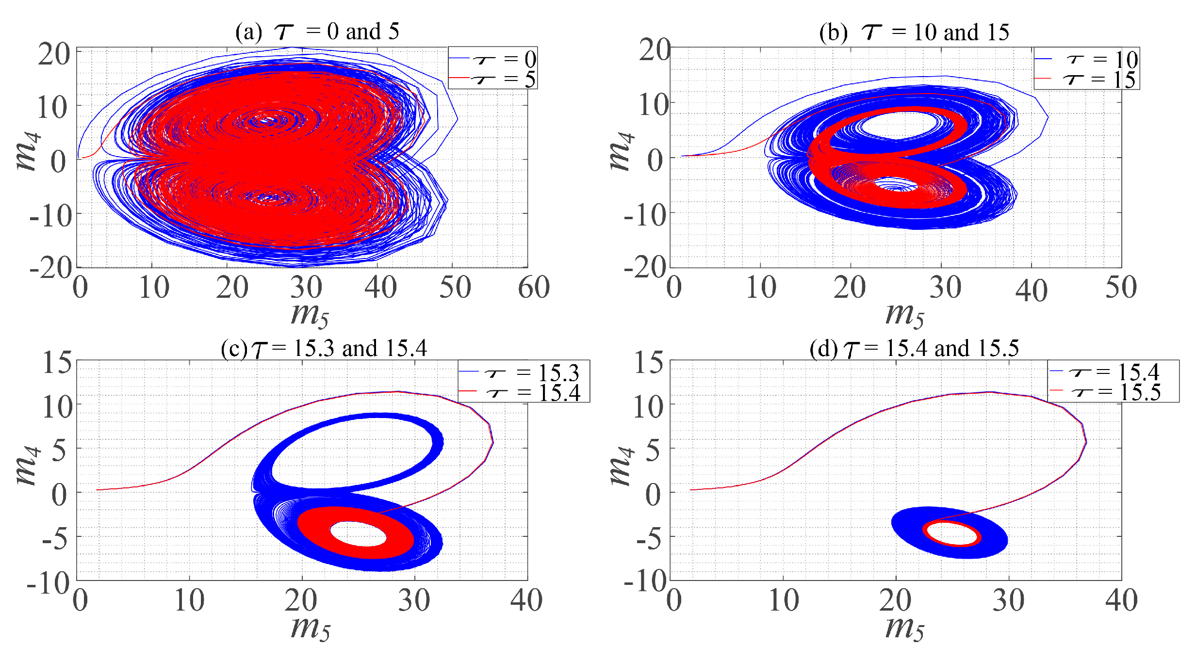
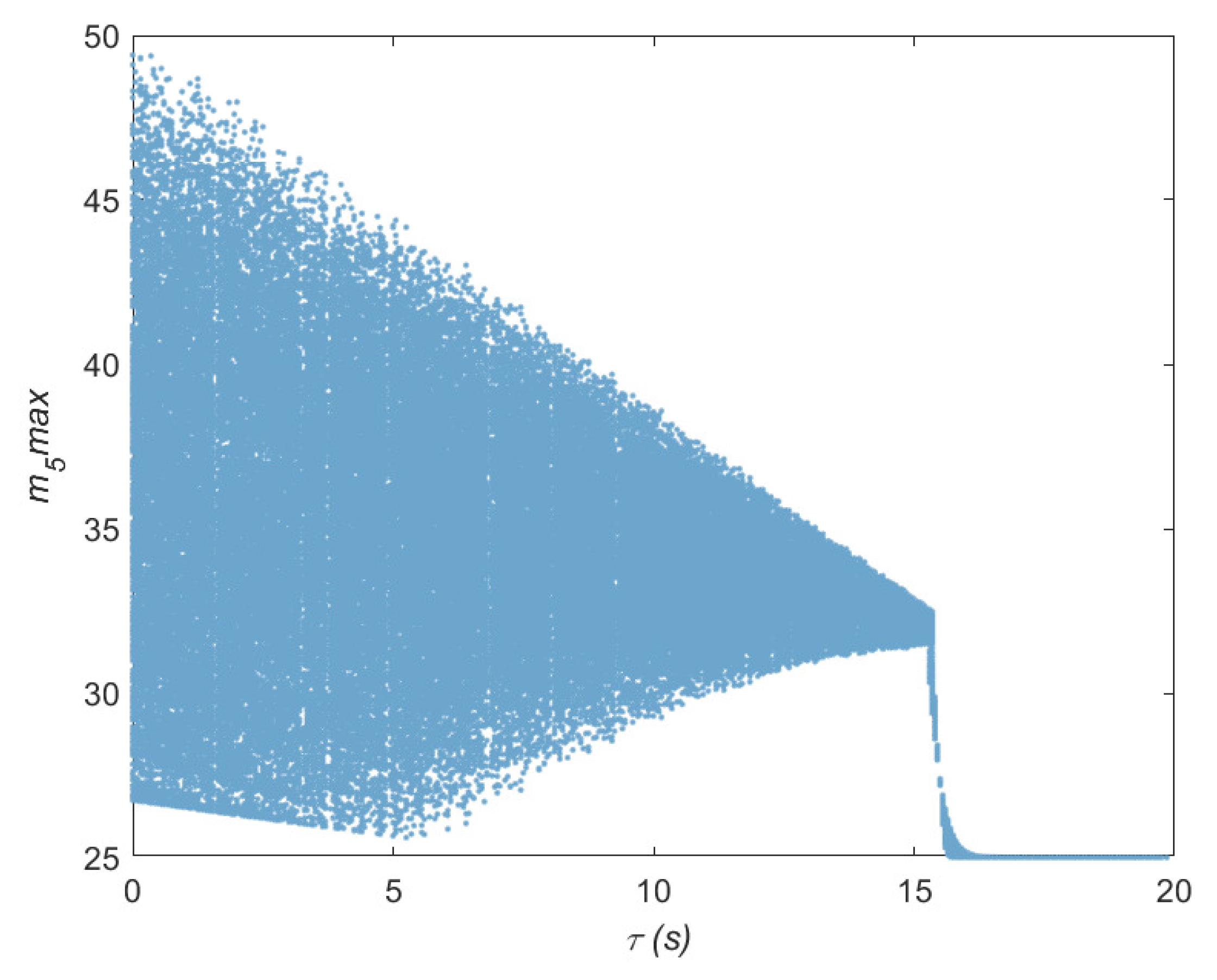
2.2. Time Chaotic Attractor

The chaotic characteristics of the time-delay fractional complex $L\ddot{u}$ system are different from the original system because the time-delay system has high randomness and an unpredictable time series [26]. When parameter $a_1=45,a_2=25,a_3=8,q_l=0.95$, the initial value is set to $m_i=(0.1,0.2,0.3,0.2,0.3)(i=1,\cdots ,5)$, the time chaotic attractor subgraphs at different time-delay is obtained. According to Figure 1, when $\tau =15.4$, the time-delay fractional complex $L\ddot{u}$ system is no longer in a chaotic state. From the bifurcation diagram in Figure 2, it can be verified that when $\tau \ge 15.4$, the system no longer appears chaotic.

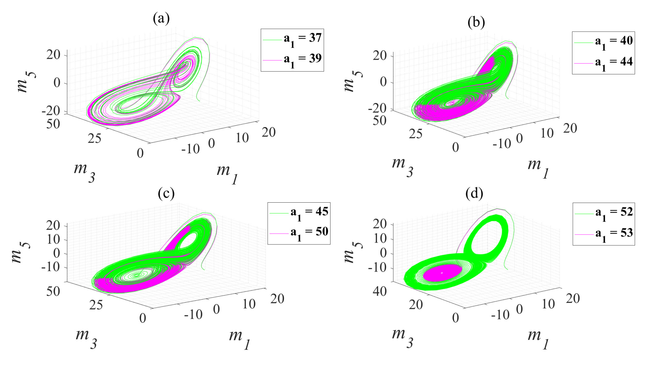
2.3. Coexistence Attractor

When the initial value of the chaotic system changes to $(m_1^{\prime },m_2^{\prime },m_3^{\prime },m_4^{\prime },m_5^{\prime },\tau )=(0.8,0.8,0,0,0,15)$ and the other parameters remain unchanged, we can get a set of coexistence attractor graphs, as shown in Figure 3, where the red chaotic attractor represents the interval $m_i^{\prime }=(0.8,0.8,0,0,0)$, and the blue chaotic attractor interval is $m_i=(0.1,0.2,0.3,0.2,0.3)$. It can be seen from Figure 3 that the coexistence attractor exists in the time-delay fractional complex $L\ddot{u}$ system [27]. It can be seen from the bifurcation diagrams in Figure 2 and Figure 4 that the change of the initial value has little effect on the time-delays. According to the sensitivity of the initial value, we can know the linear change of the initial condition. The result has no linear deviation, but the chaotic state is different. However, because the parameters and order do not change, the time-delay range of the chaotic system does not change with the change of the initial value.

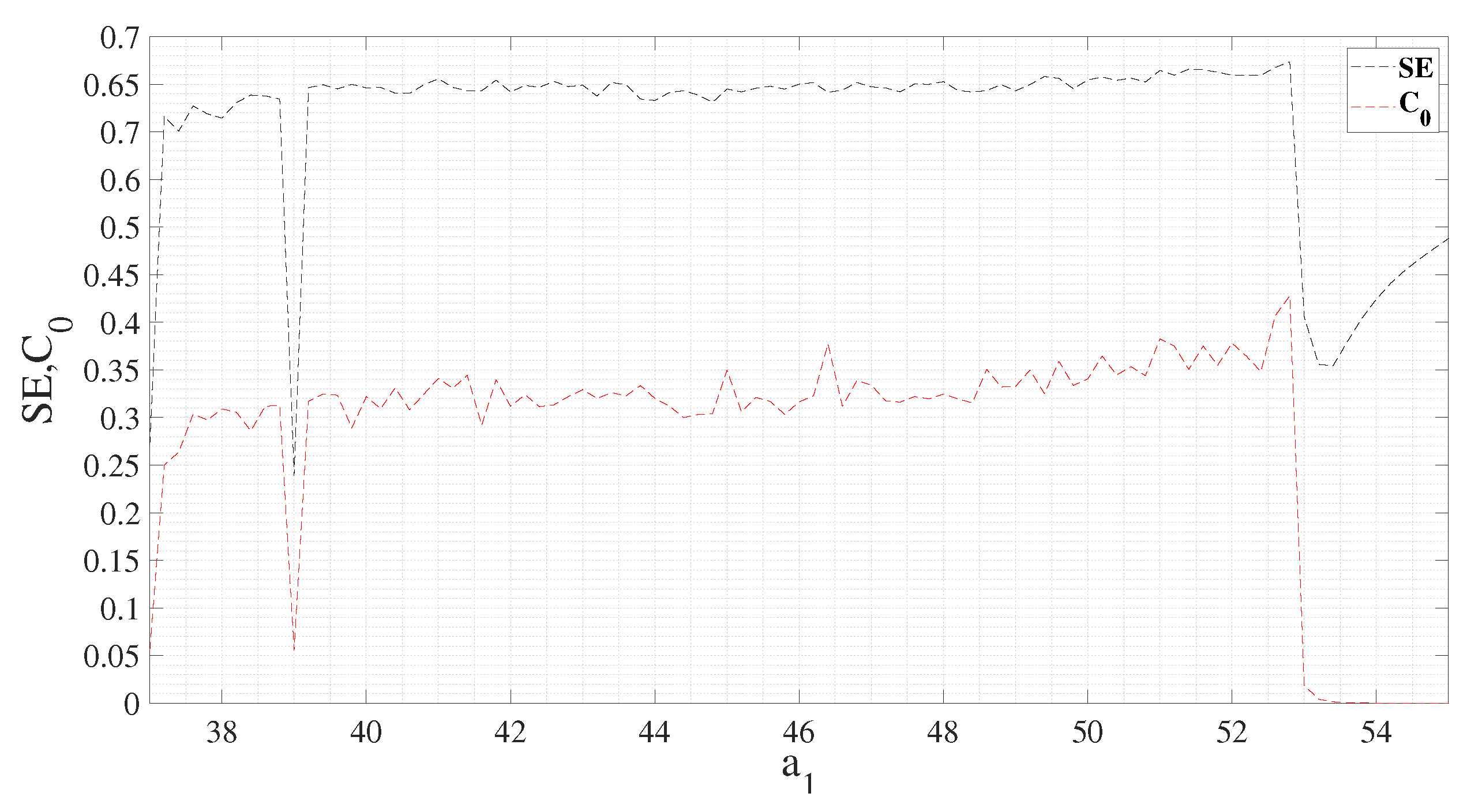
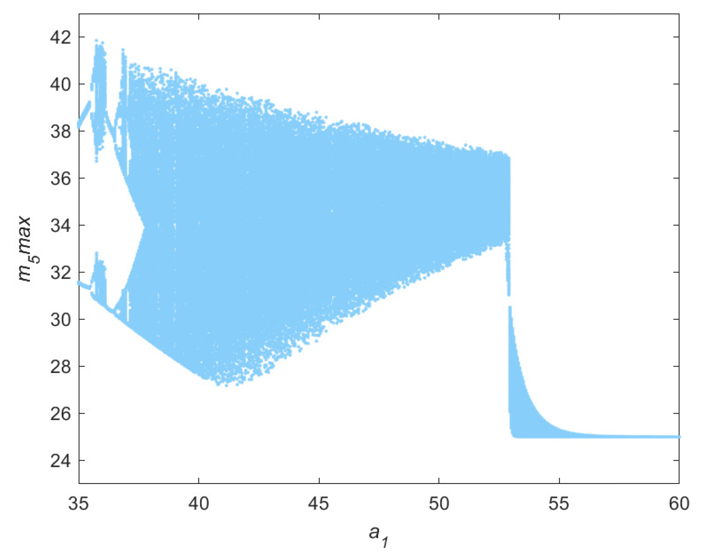
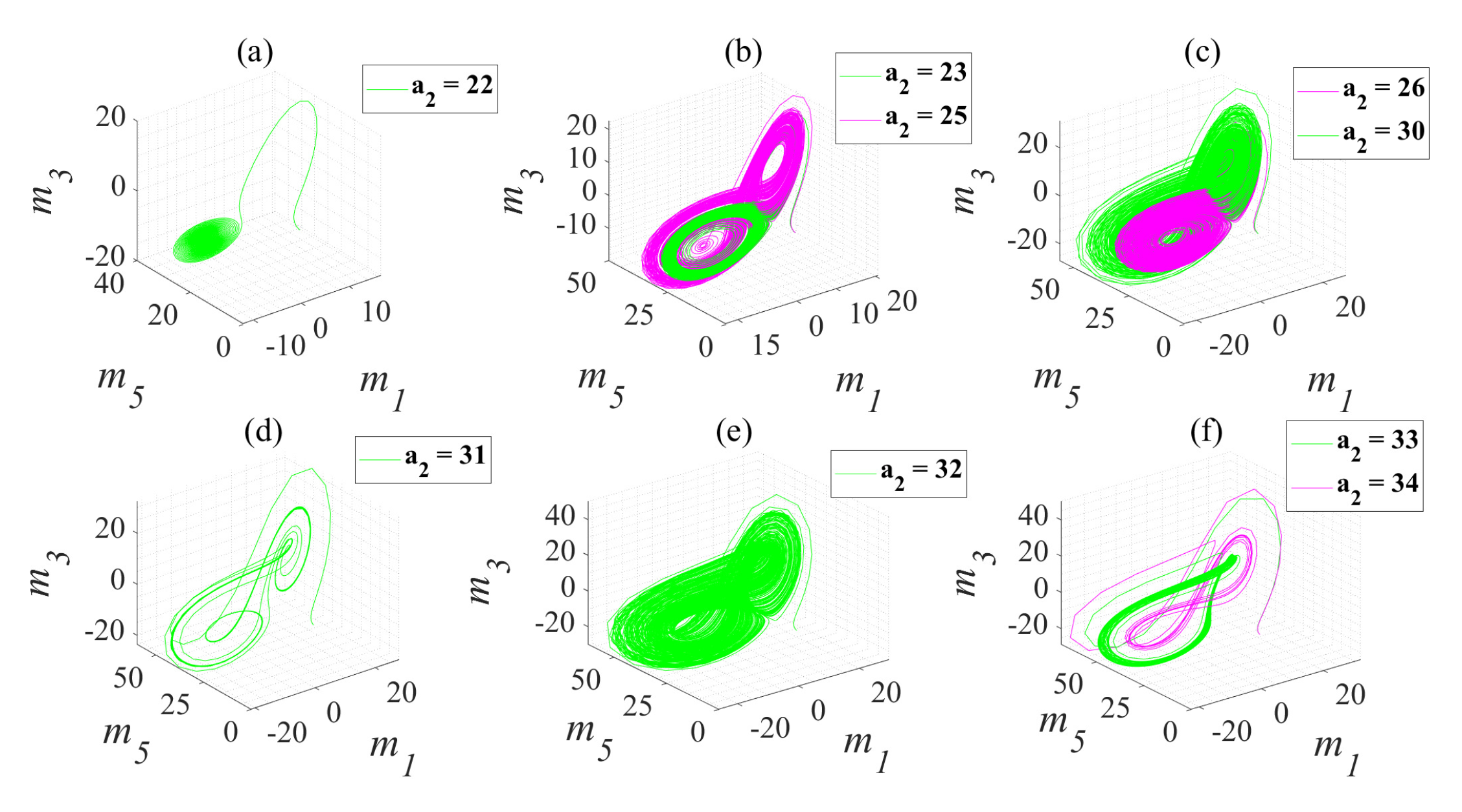
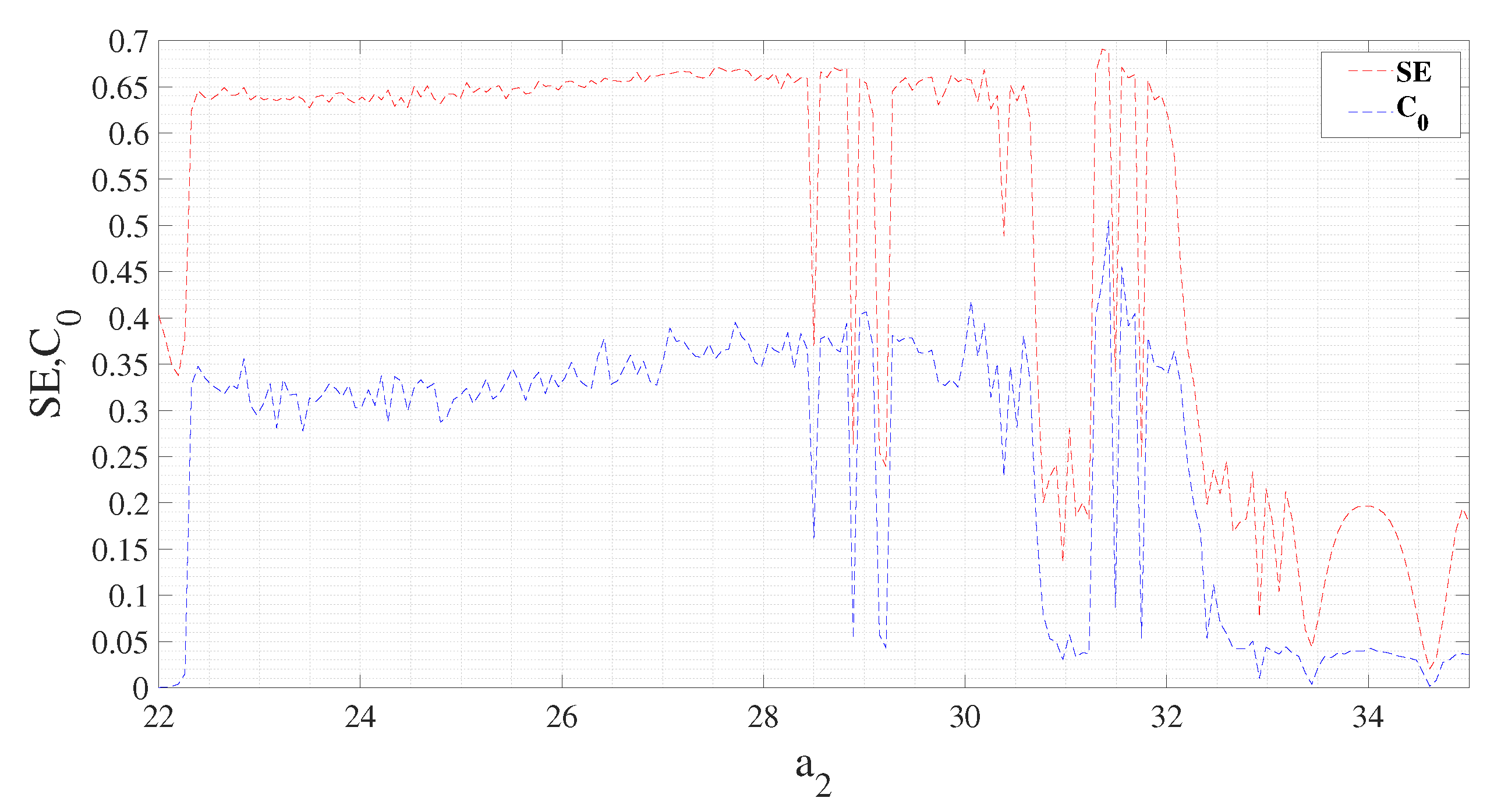
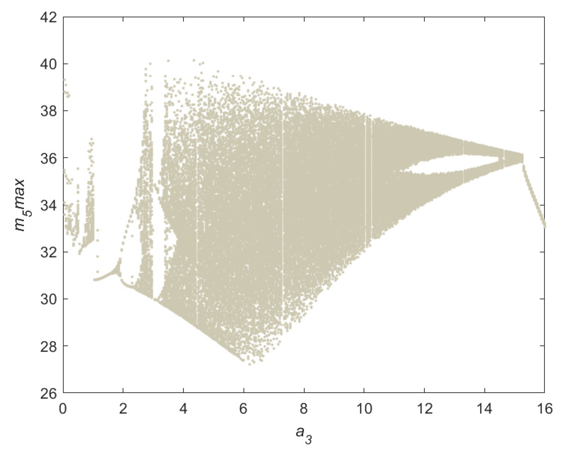
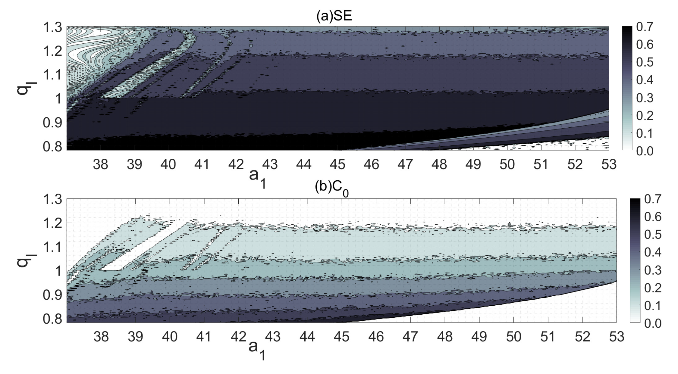
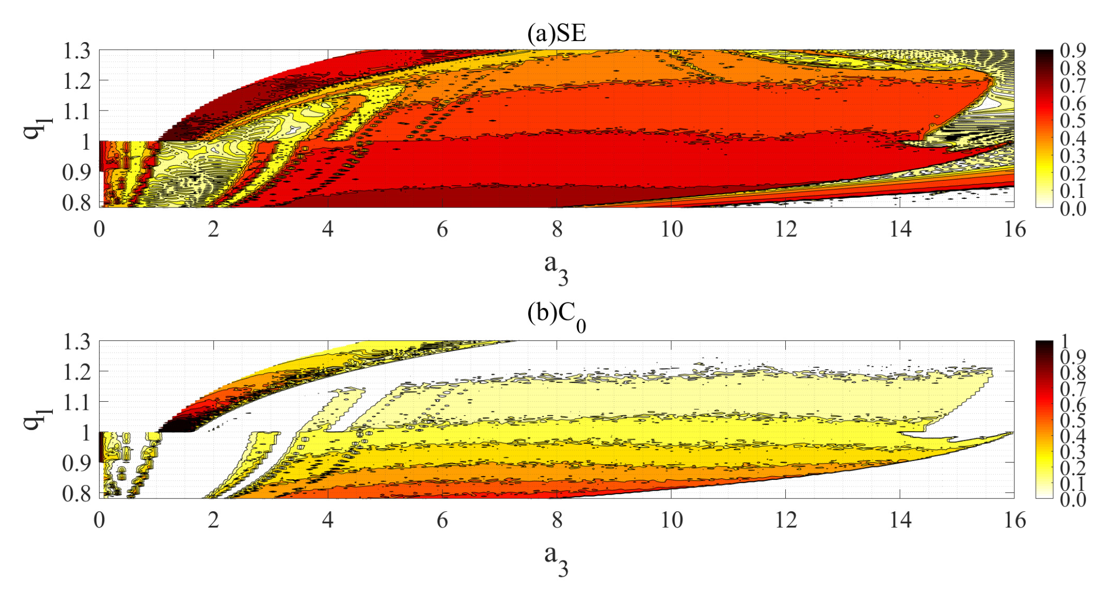
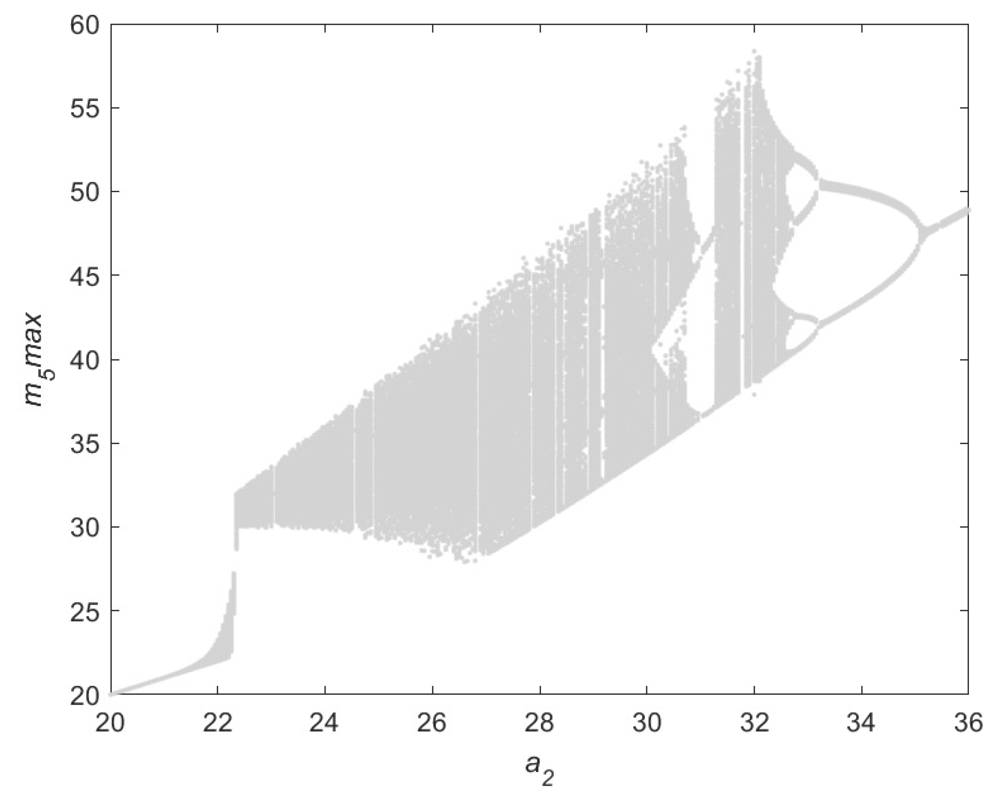
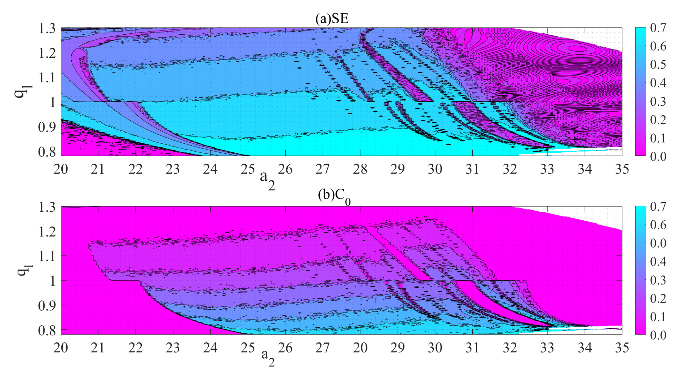
2.4. Parameter Space and Analysis of Its Chaotic Characteristics

When the initial value of the chaotic system remains unchanged and three parameters are changed, changes of the parameter space is observed. Therefore, the graphs of attractor changes under different parameters are observed when the initial value is set to $(m_1,m_2,m_3,m_4,m_5,\tau )=(0.1,0.2,0.3,0.2,0.3,10)$. Firstly, if the $a_1$ parameter is changed, and the other parameters remain unchanged, a $a_1$ parameter space chaotic attractor graph is obtained, as shown in Figure 5. The complexity that varies with parameter $a_1$, as shown in Figure 6, with the bifurcation diagram with parameter $a_1$, shown in Figure 7. From these figures, it can be observed that chaos occurs for the range of parameter $a_1\in (37,53)$. When $a_1\in (39,53)$, the value of Spectral Entropy(SE) algorithm remains nominally at about 0.64. Therefore, when designing a secure communication scheme, it should be selected within this range.

Secondly, according to the analysis method of parameter $a_1$, changing the parameter $a_2$, the second parameter space chaotic attractor graph and the complexity graph of $a_2$ can be obtained, as shown in Figure 8 and Figure 9. It can be seen that chaotic behavior is exhibited in the parameter range $a_2\in (22,33)$. According to Figure 9, the system is relatively stable in the range of $a_2\in [23,28]$, so this range from which to select the parameter $a_2$. From the bifurcation diagram in Figure 10, which varies with the parameter $a_2$, it can be concluded that the system is stable and the chaotic state is better in $a_2\in [23,28]$.

Finally, when the parameter $a_3$ is changed, the parameter space attractor graph and the complexity graph for $a_3$ can be obtained, as shown in Figure 11 and Figure 12. It can be seen that the chaos is exhibited for the range $a_3\in (2,15]$. According to Figure 12, the complexity value of the system is relatively large in the range of $a_3\in [5,15]$, the system is stable and is therefore preferred. Therefore, through the analysis bifurcation diagram in Figure 13, when $a_3\in [5,11]$, the system is stable and the chaotic state is better.

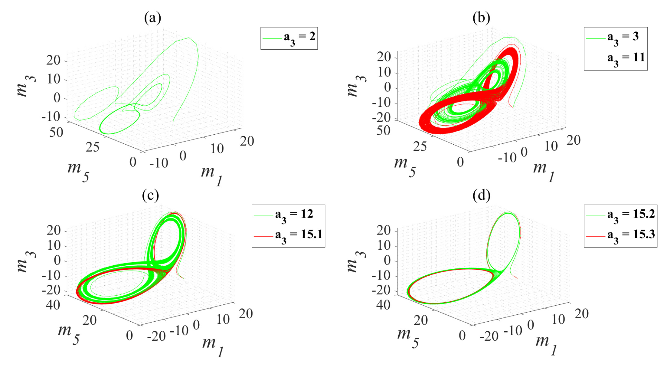
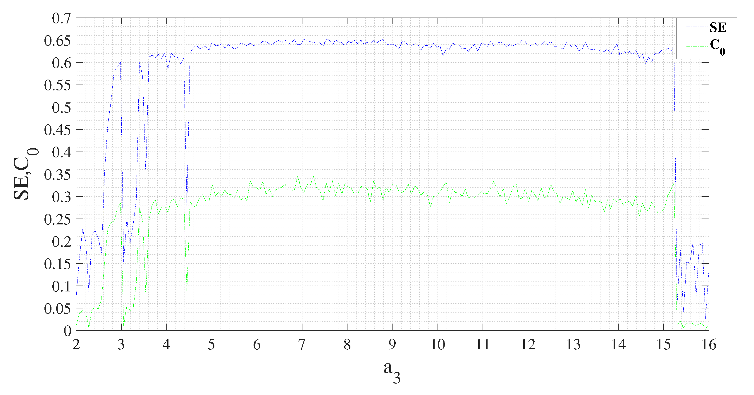
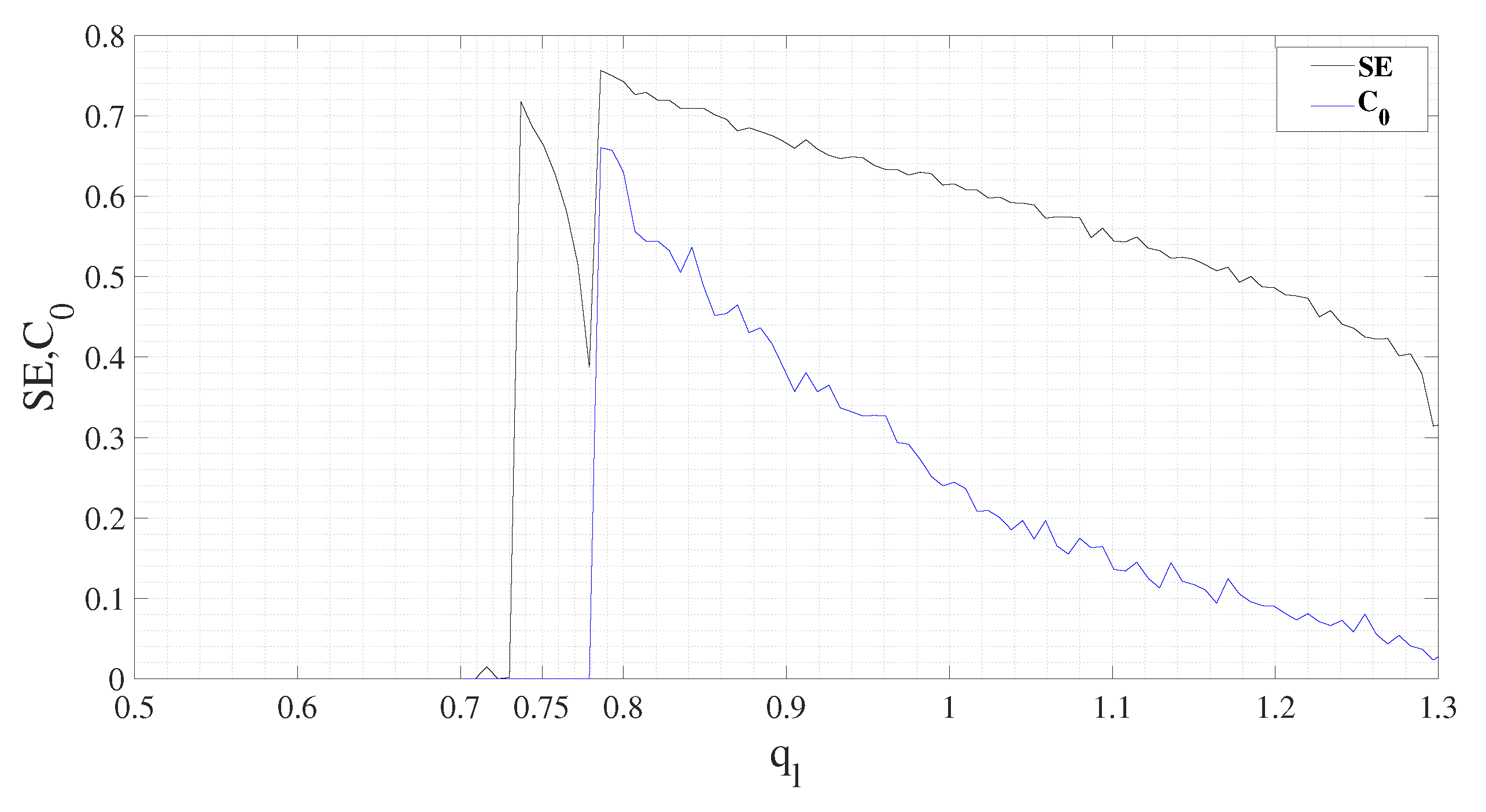
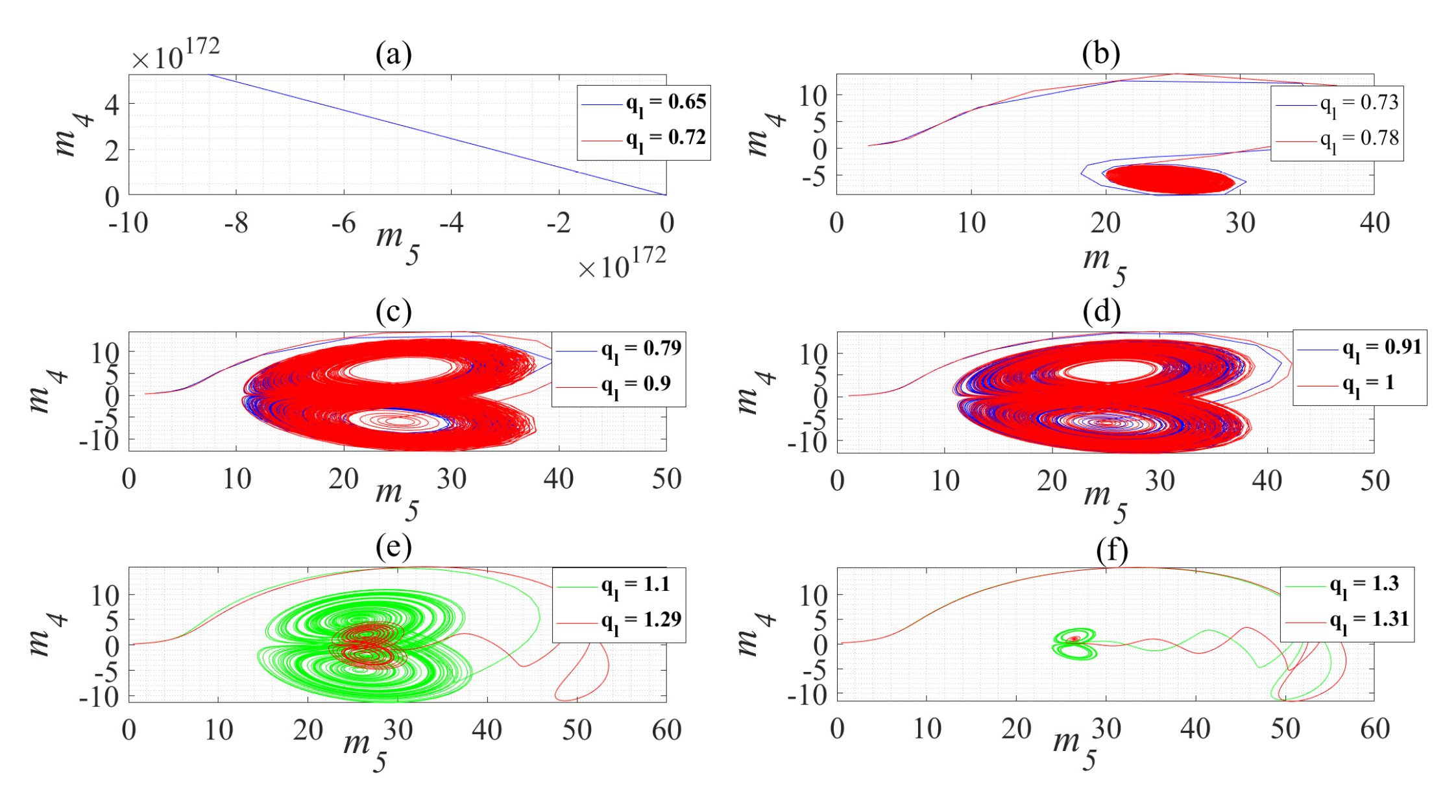
2.5. Fractional-Order Changes and Complexity Analysis

The complexity of the chaotic system is a commonly used method to describe the dynamic characteristics of the chaotic system. In this article, the SE algorithm and $C_0$ algorithm are mainly used to analyze the chaotic characteristics of the system [28]. The complexity of chaotic system indicates how to close the chaotic sequence to a random sequence. The larger the complexity value, the closer the sequence is to the random sequence, and therefore the higher the corresponding security. Next, according to the SE algorithm and the $C_0$ algorithm, the complexity of fractional-order $q_l$ is analyzed. Finally, the complexity of $q_l$ and three parameters changing simultaneously is analyzed.

Firstly,

Table 1. The dynamic state of the chaotic system at different fractional orders.

${\mathit{q}}_{\mathit{l}}$	SE	${\mathit{C}}_0$	Dynamic State
$0<q_l<0.73$	0	0	Non-chaotic
$0.73\le q_l\le 0.78$	0.71–0.38	0	Non-chaotic
$0.78<q_l\le 0.9$	0.75–0.38	0.66–0.24	Chaotic
$0.9\le q_l\le 1$	0.67–0.61	0.38–0.24	Chaotic
$1<q_l\le 1.3$	0.61–0.31	0.24–0.02	Chaotic
$q_l>1.3$	0	0	Non-chaotic

gives the range of the $SE$ and $C_0$ complexity algorithm with the order $q_l$ to determine the dynamic state of the system. When the range of complexity drops sharply, the system is no longer chaotic; when the complexity begins to slowly decrease, the system enters the chaotic state; when the value of any complexity algorithm tends to zero, the system is no longer chaotic. Table 1, Figure 14 and Figure 15 are the results obtained when $a_1=45,a_2=25,a_3=8,\tau =10$. The variation range of order $q_l$ can be intuitively observed from Figure 14 and Figure 15, when $q_l\in [0.79,1.31)$, the system is in a chaotic regime.

Secondly, according to Figure 16, the complexity changes when $q_l$ and the parameter $a_1$ change simultaneously. When $a_1\in (37,49]$, the value of SE and $C_0$ is relatively large within $q_l\in [0.78,1]$ in Figure 16. According to Figure 17, when $q_l\in [0.78,1]$ is relatively large in the range of $a_2\in (22,29)$, and the chaotic phenomenon is very obvious in its range. Figure 18 is a chaotic diagram of complexity when the chaotic system $q_l$ and $a_3$ change at the same time. According to Figure 18, the value of SE is relatively large in the range of $a_3\in [4,11]$.

3. Modified Fractional Projective Difference Function Synchronization

3.1. Definition of MFPDFS

Consider the following two time-delay fractional complex chaotic systems.

Master system: $D_{*}^{q_l}\dot{Y}\left(t\right)=g(y-\tau ),y\in R^n$.

Slave system: $D_{*}^{q_l}\dot{X}\left(t\right)=f(x-\tau ),x\in R^n$, where $\dot{Y}\left(t\right)={[y_1\left(t\right),\cdots ,y_n\left(t\right)]}^T$, $\dot{X}\left(t\right)={[x_1\left(t\right),\cdots ,x_n\left(t\right)]}^T$.

Definition 3.

For the state vectors $D_{*}^{q_l}\dot{Y}\left(t\right)$ and $D_{*}^{q_l}\dot{X}\left(t\right)$, the difference between them becomes the modified projective difference function vector, expressed as:

$$D_{*}^{q_l}\dot{h}\left(t\right)=D_{*}^{q_l}\dot{Y}\left(t\right)-P{D}_{*}^{q_l}\dot{X}\left(t\right)$$

(7)

where $D_{*}^{q_l}\dot{h}\left(t\right)=[h_1\left(t\right),\cdots ,h_n\left(t\right)]$ is the bounded complex function vector, $P=diag(p_1,\cdots ,p_n)$ is the complex scale factor matrix that can be adjusted.

Definition 4.

For two arbitrary fractional complex chaotic state vectors and the specified modified projective difference function vectors, the following conditions are satisfied:

$$\begin{array}{c}\hfill \underset{t\to \infty }{lim}{\parallel e\left(t\right)\parallel }^2=\underset{t\to \infty }{lim}\parallel D_{*}^{q_l}\dot{Y}\left(t\right)-P{D}_{*}^{q_l}\dot{X}{\left(t\right)\parallel }^2-\underset{t\to \infty }{lim}{\parallel D_{*}^{q_l}\dot{h}\left(t\right)\parallel }^2\end{array}$$

(8)

where $\parallel ·\parallel$ is the matrix norm. It is said that $D_{*}^{q_l}\dot{Y}\left(t\right)$ and $D_{*}^{q_l}\dot{X}\left(t\right)$ realize MFPDFS.

Remark 1.

When $P=0$, MFPDFS becomes fractional difference function synchronization (FDFS).

Remark 2.

When $q_l=1(l=1,2,3),P=0$, MFPDFS becomes difference function synchronization (DFS).

Remark 3.

When $D_{*}^{q_l}\dot{h}\left(t\right)=0$ and $q_l=1,P=0$, MFPDFS becomes complete synchronization (CS).

3.2. Design of the MFPDFS Controller

Given the following time-delay fractional complex $L\ddot{u}$ system as the drive system and the response system, respectively:

$$\begin{array}{c}\hfill \begin{array}{c}\left\{\begin{array}{ccc}{D}_{*}^{q_l}\dot{x}\hfill & =\hfill & Ax+F_1\left(x\right)\hfill \\ D_{*}^{q_l}\dot{y}\hfill & =\hfill & By+F_2\left(y\right)+u\hfill \\ D_{*}^{q_l}u\hfill & =\hfill & F_3(x,y)\hfill \end{array}\right.\hfill \end{array}\end{array}$$

(9)

where $D_{*}^{q_l}\dot{x}=m_1^{\prime },\cdots ,m_5^{\prime }$, $D_{*}^{q_l}\dot{y}=m_1,\cdots ,m_5$, u is the MFPDFS controller. The specific expressions of the drive system and response system are as follows:

$$\begin{array}{c}\hfill \begin{array}{c}\left\{\begin{array}{ccc}{D}_{*}^{q_1}\dot{m_1^{\prime }}\hfill & =\hfill & a_1(m_3^{\prime }-m_1^{\prime })\hfill \\ D_{*}^{q_1}\dot{m_2^{\prime }}\hfill & =\hfill & a_1(m_4^{\prime }-m_2^{\prime })\hfill \\ D_{*}^{q_2}\dot{m_3^{\prime }}\hfill & =\hfill & a_2{m}_3^{\prime }-m_1^{\prime }{m}_5^{\prime }\hfill \\ D_{*}^{q_2}\dot{m_4^{\prime }}\hfill & =\hfill & a_2{m}_4^{\prime }-m_2^{\prime }{m}_5^{\prime }\hfill \\ D_{*}^{q_3}\dot{m_5^{\prime }}\hfill & =\hfill & -a_3{m}_5^{\prime }(t-\tau )+m_1^{\prime }{m}_3^{\prime }+m_2^{\prime }{m}_4^{\prime }\hfill \end{array}\right.\hfill \end{array}\end{array}$$

(10)

$$\begin{array}{c}\hfill \begin{array}{c}\left\{\begin{array}{ccc}{D}_{*}^{q_1}\dot{m_1}\hfill & =\hfill & a_1(m_3-m_1)+u_1\hfill \\ D_{*}^{q_1}\dot{m_2}\hfill & =\hfill & a_1(m_4-m_2)+u_2\hfill \\ D_{*}^{q_2}\dot{m_3}\hfill & =\hfill & a_2{m}_3-m_1{m}_5+u_3\hfill \\ D_{*}^{q_2}\dot{m_4}\hfill & =\hfill & a_2{m}_4-m_2{m}_5+u_4\hfill \\ D_{*}^{q_3}\dot{m_5}\hfill & =\hfill & -a_3{m}_5(t-\tau )+m_1{m}_3+m_2{m}_4+u_5.\hfill \end{array}\right.\hfill \end{array}\end{array}$$

(11)

According to [29], the lemma holds.

Lemma 1.

A fractional chaotic system is given:

$$D_{*}^{q_l}m\left(t\right)=Qm\left(t\right),m\left(0\right)=m_0$$

(12)

where $m\in R^n$, $Q\in R^{n\times n}$, and $0<q_l<1$. If all the eigenvalues λ of the system matrix Q are satisfied,

$$\left|arg\right(\lambda \left)\right|>q\pi /2$$

(13)

the fractional nonlinear system (12) is asymptotically stable.

We are now in a position to state and prove the following important result.

Theorem 1.

For system (9), the difference function $D_{*}^{q_l}\dot{h}$ and initial values $\dot{x}\left(0\right),\dot{y}\left(0\right)$ they jointly complete the MFPDFS, we design the controller as:

$$u=PAx-By+P{F}_1\left(x\right)-F_2\left(y\right)+D_{*}^{q_l}\dot{h}+ke$$

(14)

where k is the feedback matrix, and e is the error feedback matrix.

According to Definition 4, the error system can be expressed as:

$$e\left(t\right)=D_{*}^{q_l}\dot{y}-P{D}_{*}^{q_l}\dot{x}-D_{*}^{q_l}\dot{h}.$$

(15)

The specific MFPDFS controller expression is as follows,

$$\begin{array}{c}\hfill \begin{array}{c}\left\{\begin{array}{ccc}{u}_1\hfill & =\hfill & -a_1{e}_3+k_1{e}_1+h_1\hfill \\ u_2\hfill & =\hfill & -a_1{e}_4+k_2{e}_2+h_2\hfill \\ u_3\hfill & =\hfill & -a_2{e}_3+m_1{m}_5-P{m}_1^{\prime }{m}_5^{\prime }+k_3{e}_3+h_3\hfill \\ u_4\hfill & =\hfill & -a_2{e}_4+m_2{m}_5-P{m}_2^{\prime }{m}_5^{\prime }+k_4{e}_4+h_4\hfill \\ u_5\hfill & =\hfill & -a_3{e}_5-m_1{m}_3+P{m}_1^{\prime }{m}_3^{\prime }-m_2{m}_4+P{m}_2^{\prime }{m}_4^{\prime }+k_5{e}_5+h_5\hfill \end{array}\right.\hfill \end{array}\end{array}$$

(16)

where $e_i\left(t\right)=m_i\left(t\right)-p_i{m}_i^{\prime }\left(t\right)$, and $e_5\left(t\right)=m_5(t-\tau )-p_5{m}_5^{\prime }(t-\tau )$.

Proof of Theorem 1. 

The specific error system expression is as follows,

$$\begin{array}{c}\hfill \begin{array}{c}\left\{\begin{array}{ccc}\dot{e_1}\hfill & =\hfill & (k_1-a_1)e_1\hfill \\ \dot{e_2}\hfill & =\hfill & (k_2-a_1)e_2\hfill \\ \dot{e_3}\hfill & =\hfill & k_3{e}_3\hfill \\ \dot{e_4}\hfill & =\hfill & k_4{e}_4\hfill \\ \dot{e_5}\hfill & =\hfill & k_5{e}_5.\hfill \end{array}\right.\hfill \end{array}\end{array}$$

(17)

According to Lemma 1, the parameter matrix k needs to satisfy $\left|\arg \right(\mathrm{eig}\left(k\right)\left)\right|>q\pi /2$, where $\mathrm{eig}\left(k\right)=\lambda$ is all the eigenvalues of the parameter matrix. In order to verify the stability of the controller, the controller (14) is substituted into formula (15):

$$\begin{array}{ccc}\hfill e\left(t\right)& =& By+F_2\left(y\right)-PAx-P{F}_1\left(x\right)-D_{*}^{q_l}\dot{h}\hfill \\ & & +PAx-By+P{F}_1\left(x\right)-F_2\left(y\right)\hfill \\ & & +D_{*}^{q_l}\dot{h}+ke\hfill \\ & =& ke.\hfill \end{array}$$

(18)

Therefore, the error system (17) is asymptotically stable. System (10), system (11), and controller (16) realize MFPDFS together. □

4. Speech Secure Communication Scheme

Due to the wideband characteristics of the chaotic system, the randomness of the chaotic output can be used to cover up the useful information signal. The block diagram of the communication scheme is given in this section. Wireless speech communication is easy to be monitored in the process of transmission. Therefore, the confidentiality of WSCs is important. Figure 19 shows the specific composition of the WSCs secure block diagram and the role of each part. At the sending end of the communication systems, the signal to be communicated $M\left(t\right)$ (classic music ‘corner’ segment) is given, assuming $N\left(t\right)$ to be the interference signal that may appear during the transmission. The L1 system (10) is used as the encryption system at the transmitting end, and the L2 system (11) is used as the decryption system at the receiving end to restore the original information signal. The signal during transmission is called $S\left(t\right)$. It is expressed as $S\left(t\right)=D_{*}^{q_l}{m}_i^{\prime }\left(t\right)+M\left(t\right)+N\left(t\right)$. $Others\left(t\right)$ represent other channels that can be selected. Since the given system is a five-dimensional chaotic system, we have five channels when selecting signal transmission. After that, we will present a number of experimental demonstrations to determine a more stable channel for transmission. Assuming that when there are many audio transmissions, five channels are selected for simultaneous transmission. The MFPDFS controller (16) is used as the secure communication controller in the signal transmission process.

Compared with the communication scheme designed by the fractional real chaotic $L\ddot{u}$ system, the fractional complex chaotic $L\ddot{u}$ system can expand from three to five channels during speech transmission. In the test, the signal-noise ratio (SNR) is greater than the real chaotic $L\ddot{u}$ system, which shows that the fractional complex chaotic $L\ddot{u}$ system is more robust. The proposed secure communication scheme based on the time-delay fractional complex $L\ddot{u}$ system has the following advantages: (1) The fractional complex chaotic system not only considers the fractional domain but also combines the complex number domain, and the robustness of the system can be improved by increasing the complex scale factor;

(2) In our communication scheme, we use an MFPDFS controller to ensure that the receiving end signal is equal to the addition of the plaintext signal and the fractional complex chaotic signal;

(3) In the transmission process, one of the five channels is randomly selected, and the possibility of an eavesdropper to obtain the original information signal is very small, which greatly improves the security of communication.

All these advantages have been verified by numerical simulation, and the simulation results are given in the next section.

5. Numerical Simulation Experiment

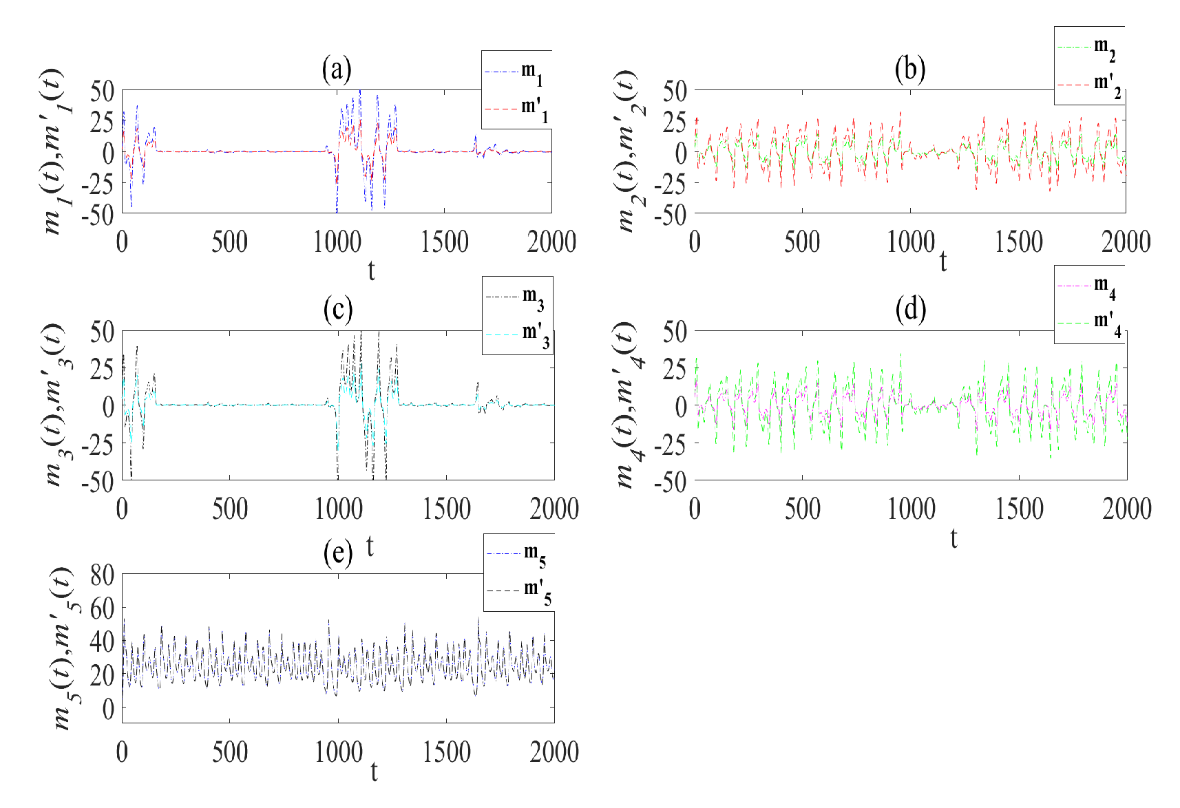
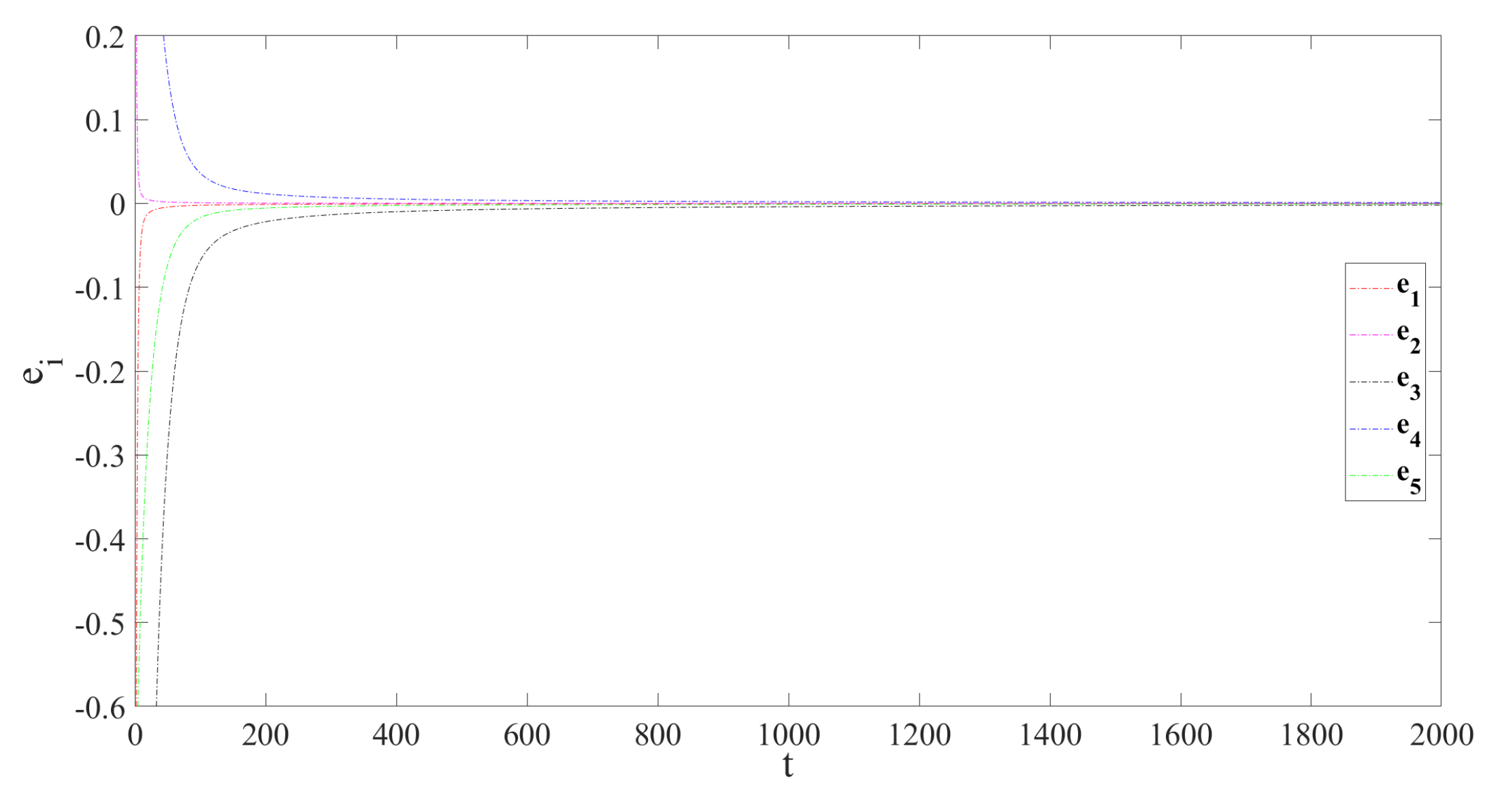
5.1. MFPDFS Controller Simulation Experiment

In order to verify the feasibility of the proposed MFPDFS controller, we discuss the MFPDFS of the time-delay fractional complex $L\ddot{u}$ system.

Based on the analysis of the dynamic characteristics above, the parameter of the system is set to $(a_1,a_2,a_3,\tau ,q_l)=(45,25,8,2,0.95)$, and the initial value of the systems are $m_i=(1,2,3,4,5)$, and $m_i^{\prime }=(1.5,2.3,3.1,4.6,5.8)$. The MFPDFS controller (16) is selected, where the complex scale factor $P=(2+j0.5,2+j0.5,1)$, the feedback parameter $k_i=-5$, and $h_i$ is the difference function factor. The state observation diagram and error feedback state diagram of the MFPDFS between the two systems are obtained through numerical simulation as shown in Figure 20 and Figure 21.

5.2. SNR Test Experiment

In this section, according to formula (19) of SNR, the SNR of the first channel of speech transmission is given.

$$SNR=10{\log }_{10}\left(\frac{P_s}{P_n}\right)$$

(19)

where $P_n=P_s-P_s^{\prime }$, $P_s^{\prime }$ is the restored speech signal adjusted by the scale factor $p_1$.

The channel R1 represents the first transmission channel that is used in this article to transmit signals, $p_1$ is the scale factor that can be adjusted, $P_s$ is the effective power value of the original speech signal, $P_n$ is the effective power value of the noise signal, and SNR represents the signal-to-noise ratio after audio noise reduction.

It can be seen from

Table 2. Analysis of SNR under different scale factors.

${\mathit{p}}_1$	${\mathit{P}}_{\mathit{s}}$	${\mathit{P}}_{\mathit{n}}$	SNR
0.5	292.9168	0.0325	39.5465
0.8	292.9168	0.0208	41.4847
0.9	292.9168	0.0637	36.6239
1	292.9168	0.1301	33.5259
1.5	292.9168	0.8129	25.5671

and

Table 3. Analysis of SNR of the fractional real $L\ddot{u}$ system under different scale factors.

${\mathit{p}}_1$	${\mathit{P}}_{\mathit{s}}$	${\mathit{P}}_{\mathit{n}}$	SNR
0.5	292.9168	0.0393	38.7253
0.8	292.9168	0.0356	39.1553
0.9	292.9168	0.0989	34.7150
1	292.9168	0.1945	31.7777
1.5	292.9168	1.1568	24.0348

that at $p_1=0.8$, the SNR of the two systems are both at maximum, but the SNR of the fractional complex $L\ddot{u}$ system is slightly higher than the fractional real $L\ddot{u}$ system. In this scheme, the robustness of fractional complex $L\ddot{u}$ system is slightly better.

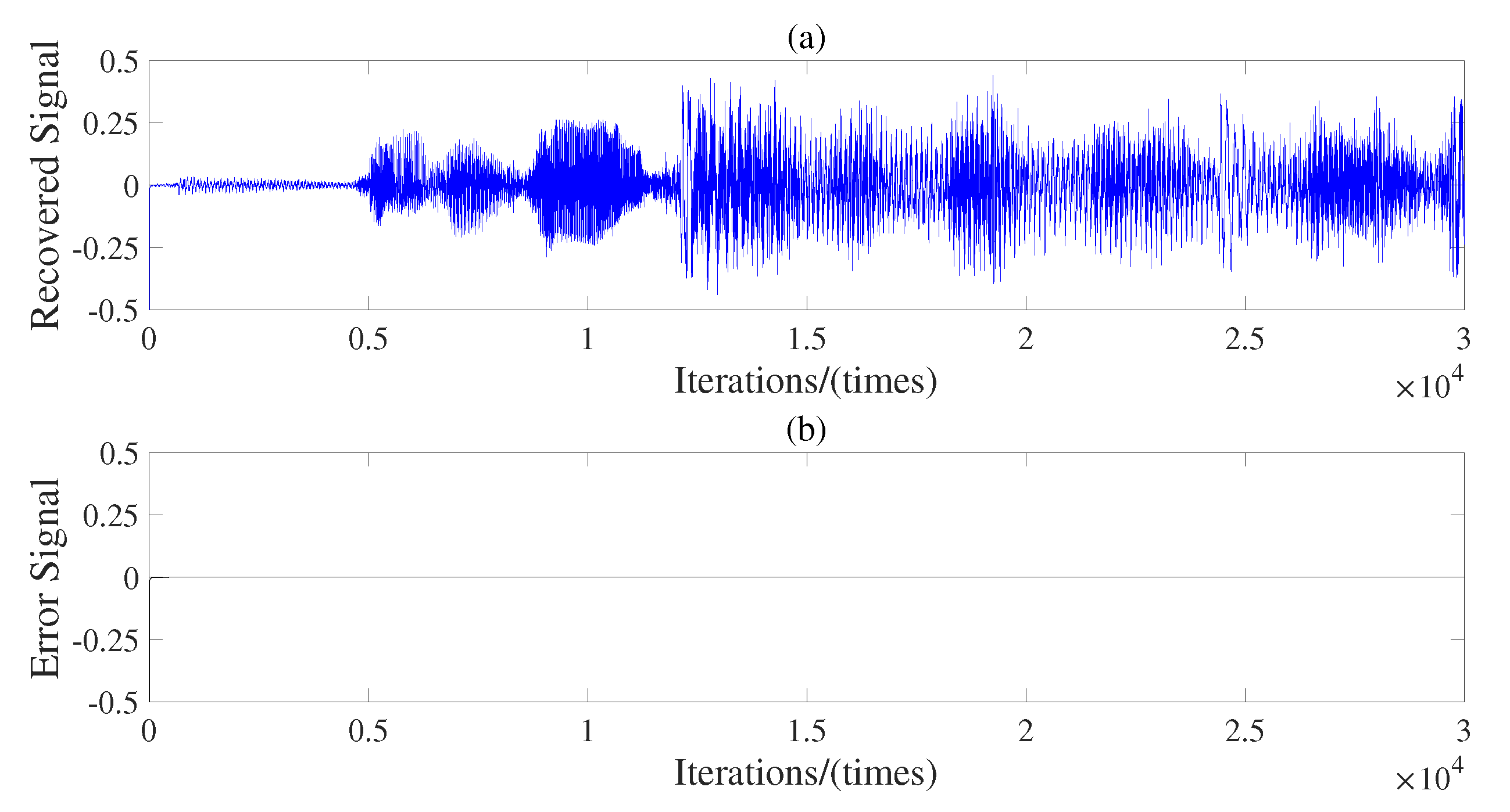
5.3. Speech Communication Simulation

In order to verify the security of the proposed WSCs security system, we use the drive system (10) as the L1 system, the response system (11) as the L2 system, and the MFPDFS controller (16) as the controller of this communication scheme. The difference function factor $h_i$ represents the information signal $M\left(t\right)=(h_1,\cdots ,h_5)$. The complex scale factor is $P=(0.8+j2,0.8+j2,1)$, and the time-delay is $\tau =2$. The initial value of the system is set to $m_i=(1,2,3,4,5)$ and $m_i^{\prime }=(1.5,2.5,3.5,4.2,5.2)$.

A piece of audio is used to transmit the speech signal, which is converted into a waveform signal for encryption and decryption during transmission. Since there are five communication channels that can provide transmission in this communication scheme, the first channel to transmit the signal is chosen. The waveform diagram of the original speech signal is shown in Figure 22a, the transmitted signal in the encryption process is shown in Figure 22b. According to Figure 22b, the encrypted transmission signal has completely covered the original sound signal, and unauthorized third parties have no chance to extract the original sound information from the transmission signal. This fully proves the high confidentiality of the system for sound signal transmission. The waveform diagram of the restored voice signal is shown in Figure 23a. The original signal and the error state change diagram of the restored signal is shown in Figure 23b. Finally, it can be seen from Figure 23 that the recovered signal is exactly the same as the original signal, and the error is zero.

6. Conclusions

In this paper, the differential equations of a time-delay fractional order complex $L\ddot{u}$ system is given. The dynamic characteristics of the system are analyzed by a bifurcation diagram and complexity algorithm. At the same time, it is concluded that the complexity of a fractional order complex chaotic system decreases with the increase of fractional order in a certain range, and remains high with the change of parameters in a certain range. The results show that the fractional order time-delay system has rich dynamic characteristics, so it can be applied to speech secure communication. According to the new synchronization mode proposed in this paper, a synchronization controller is designed. The stable output value is obtained by adjusting the scale factor. After testing, the speech signal is perfectly recovered.

In this paper, the shortcomings relate to a need for more specific security attack testing and circuit hardware implementation. Our next step is to implement a chaotic circuit on FPGA and analyze it more specifically.

References

1. Gao, X.; Yu, J.B. Chaos in the fractional order periodically forced complex Duffing’s oscillators. Chaos Solitons Fractals 2005, 26, 1097–1104. [Google Scholar] [CrossRef]
2. Reza, B.; Ali, B.M. Synchronization of different fractional order chaotic systems with time-varying parameter and orders. ISA Trans. 2018, 80, 399–410. [Google Scholar]
3. Chai, L.; Liu, J.; Chen, G.; Zhao, X. Dynamics and synchronization of a complex-valued star network. Sci. China Technol. Sci. 2021, 64, 2729–2743. [Google Scholar] [CrossRef]
4. Liu, J.; Chen, G.; Zhao, X. Generalized synchronization and parameters identification of different-dimensional chaotic systems in the complex field. Fractals 2021, 29, 2150081. [Google Scholar] [CrossRef]
5. Zhao, X.; Liu, J.; Zhang, F.; Jiang, C. Complex generalized synchronization in complex-variable chaotic system. Eur. Phys.-J.-Spec. Top. 2021, 230, 2035–2041. [Google Scholar] [CrossRef]
6. Zheng, Y. Fuzzy prediction-based feedback control of fractional order chaotic systems. Optik 2015, 126, 5645–5649. [Google Scholar] [CrossRef]
7. Li, R.; Wu, H. Secure communication on fractional-order chaotic systems via adaptive sliding mode control with teaching–learning–feedback-based optimization. Nonlinear Dyn. 2019, 95, 1221–1243. [Google Scholar] [CrossRef]
8. Jiang, J.; Cao, D.; Chen, H. Sliding mode control for a class of variable-order fractional chaotic systems. J. Frankl. Inst. 2020, 357, 10127–10158. [Google Scholar] [CrossRef]
9. Wu, X.; Bao, H.; Cao, J. Finite-time inter-layer projective synchronization of Caputo fractional-order two-layer networks by sliding mode control. J. Frankl. Inst. 2020, 358, 1002–1020. [Google Scholar] [CrossRef]
10. Chan, J.; Lee, T.H.; Tan, C.P. Secure Communication Through a Chaotic System and a Sliding-Mode Observer. IEEE Trans. Syst. Man Cybern. Syst. 2020, 99, 1–13. [Google Scholar] [CrossRef]
11. Khettab, K.; Ladaci, S.; Bensafia, Y. Fuzzy adaptive control of fractional order chaotic systems with unknown control gain sign using a fractional order Nussbaum gain. IEEE/ CAA J. Autom. Sin. 2019, 6, 816–823. [Google Scholar] [CrossRef]
12. Pisarchik, A.; Jaimes-Reátegui, R.; Rodríguez-Flores, C.; García-López, J.; Huerta-Cuellar, G.; Martín-Pasquín, F. Secure chaotic communication based on extreme multistability. J. Frankl. Inst. 2021, 358, 2561–2575. [Google Scholar] [CrossRef]
13. Bendoukha, S.; Abdelmalek, S. The fractional chua chaotic system: Dynamics, synchronization, and application to secure communications. Int. J. Nonlinear Sci. Numer. Simul. 2019, 20, 77–88. [Google Scholar] [CrossRef]
14. Liu, J.; Wang, Z.; Shu, M.; Zhang, F.; Leng, S.; Sun, X. Secure Communication of Fractional Complex Chaotic Systems Based on Fractional Difference Function Synchronization. Complexity 2019, 2019, 7242791. [Google Scholar] [CrossRef] [Green Version]
15. Zhang, L.; Sun, K.; Liu, W.; He, S. A novel color image encryption scheme using fractional-order hyperchaotic system and DNA sequence operations. Chin. Phys. B 2017, 26, 98–106. [Google Scholar] [CrossRef]
16. Lai, Q.; Norouzi, B.; Liu, F. Dynamic analysis, circuit realization, control design and image encryption application of an extended Lü system with coexisting attractors. Chaos Solitons Fractals 2018, 114, 230–245. [Google Scholar] [CrossRef]
17. Wang, R.; Zhang, Y.; Chen, Y.; Chen, X.; Xi, L. Fuzzy neural network-based chaos synchronization for a class of fractional-order chaotic systems: An adaptive sliding mode control approach. Nonlinear Dyn. 2020, 100, 1275–1287. [Google Scholar] [CrossRef]
18. Bhatnagar, G.; Wu, Q. Biometric Inspired Multimedia Encryption Based on Dual Parameter Fractional Fourier Transform. IEEE Trans. Syst. Man Cybern. Syst. 2014, 44, 1234–1247. [Google Scholar] [CrossRef]
19. Cai, X.; Xu, W.; Wang, L.; Chen, G. Towards High-Data-Rate Noncoherent Chaotic Communication: A Multiple-Mode Differential Chaos Shift Keying System. IEEE Trans. Wirel. Commun. 2021, 20, 4888–4901. [Google Scholar] [CrossRef]
20. Luo, C.; Wang, X. Chaos in the fractional-order complex Lorenz system and its synchronization. Nonlinear Dyn. 2013, 71, 241–257. [Google Scholar] [CrossRef]
21. Luo, C.; Wang, X. Chaos generated from the fractional-order complex Chen system and its application to digital secure communication. Int. J. Mod. Phys. C 2013, 24, 1350025–1350047. [Google Scholar] [CrossRef]
22. Liu, X.; Hong, L.; Yang, L. Fractional-order complex T system: Bifurcations, chaos control, and synchronization. Nonlinear Dyn. 2013, 75, 589–602. [Google Scholar] [CrossRef]
23. Jiang, C.; Liu, S.; Luo, C. A New Fractional-Order Chaotic Complex System and Its Anti-synchronization. Abstr. Appl. Anal. 2014, 2014, 326354. [Google Scholar] [CrossRef]
24. Caputo, M. Linear models of dissipation whose Q is almost frequency independent-II. Geophys. J. R. Astron. Soc. 1967, 13, 529–539. [Google Scholar] [CrossRef]
25. Adomian, G. A new approach to nonlinear partial differential equations. J. Math. Anal. Appl. 1984, 102, 420–434. [Google Scholar] [CrossRef] [Green Version]
26. Lei, T.; He, J.; Fu, H.; Dai, W. Dynamics analysis of fractional-order Lü chaotic system with time-delay based on adomian decomposition. Sci. Technol. Eng. 2020, 20, 12711–12716. [Google Scholar]
27. Zhao, X.; Liu, J.; Liu, H.; Zhang, F. Solution of the fractional-order chaotic system based on Adomian decomposition algorithm and its complexity analysis. IEEE Access 2020, 8, 28774–28781. [Google Scholar] [CrossRef]
28. He, S.; Sun, K.; Wang, H. The Adomian Decomposition Method of Fractional Chaotic System and Its Complexity Analysis. Acta Phys. Sin. 2014, 63, 030502-72. Available online: https://kns.cnki.net/kcms/detail/detail.aspx?dbcode=CJFD&dbname=CJFD2014\&filename=WLXB201403008&uniplatform=NZKPT&v=V24QuWTxDUAhbliYoNbKsbw7oINjDjLglTLqZwfnxRC8cuBJFzuDArofKIvV_Ghj (accessed on 11 November 2021).
29. Matignon, D. Stability results for fractional differential equations with applications to control processing. Comput. Eng. Syst. Appl. 1996, 2, 963–968. [Google Scholar]
Figure 1. Chaotic attractors associated with different time-delays.
Mathematics 09 03305 g001
Figure 2. Bifurcation diagram with different time-delays ( m i ) .
Mathematics 09 03305 g002
Figure 3. When τ = 15 coexistence attractor graphs.
Mathematics 09 03305 g003
Figure 4. Bifurcation diagram with different time-delays ( m i ) .
Mathematics 09 03305 g004
Figure 5. Parametric attractor graphs of a 1 . (a) different parametric attractor graphs a 1 = 37 and a 1 = 39 ; (b) different parametric attractor graphs a 1 = 40 and a 1 = 44 ; (c) different parametric attractor graphs a 1 = 45 and a 1 = 50 ; (d) different parametric attractor graphs a 1 = 52 and a 1 = 53 .
Mathematics 09 03305 g005
Figure 6. When a 2 = 25 , a 3 = 8 , q l = 0.95 , τ = 10 , the complexity of the Spectral Entropy (SE) algorithm and C 0 algorithm varies with parameter a 1 .
Mathematics 09 03305 g006
Figure 7. When a 2 = 25 , a 3 = 8 , q l = 0.95 , τ = 10 , the bifurcation diagram varies with parameter a 1 .
Mathematics 09 03305 g007
Figure 8. Parametric attractor graphs of a 2 . (a) parametric attractor graph a 2 = 37 ; (b) different parametric attractor graphs a 2 = 23 and a 2 = 25 ; (c) different parametric attractor graphs a 2 = 26 and a 1 = 30 ; (d) parametric attractor graph a 2 = 31 ; (e) parametric attractor graph a 2 = 32 ; (f) different parametric attractor graphs a 2 = 33 and a 2 = 34 .
Mathematics 09 03305 g008
Figure 9. When a 1 = 45 , a 3 = 8 , q l = 0.95 , τ = 10 , the complexity of the SE algorithm and C 0 algorithm varies with parameter a 2 .
Mathematics 09 03305 g009
Figure 10. When a 1 = 45 , a 3 = 8 , q l = 0.95 , τ = 10 , the bifurcation diagram of varies with parameter a 2 .
Mathematics 09 03305 g010
Figure 11. Parametric attractor graphs of a 3 . (a) parametric attractor graphs a 3 = 2 ; (b) different parametric attractor graphs a 3 = 3 and a 3 = 11 ; (c) different parametric attractor graphs a 3 = 12 and a 3 = 15.1 ; (d) different parametric attractor graphs a 3 = 15.2 and a 3 = 15.3 .
Mathematics 09 03305 g011
Figure 12. When a 1 = 45 , a 2 = 25 , q l = 0.95 , τ = 10 , the complexity of the SE algorithm and C 0 algorithm varies with parameter a 3 .
Mathematics 09 03305 g012
Figure 13. When a 1 = 45 , a 2 = 25 , q l = 0.95 , τ = 10 , the bifurcation diagram varies with parameter a 3 .
Mathematics 09 03305 g013
Figure 14. When a 1 = 45 , a 2 = 25 , a 3 = 8 , τ = 10 , the complexity varies with q l .
Mathematics 09 03305 g014
Figure 15. The chaotic attractor graphs varying with fractional order q l . (a) the chaotic attractor graphs of q l = 0.65 and q = 0.72 ; (b) the chaotic attractor graphs of q = 0.73 and q = 0.78 ; (c) the chaotic attractor graphs of q = 0.79 and q = 0.9 ; (d) the chaotic attractor graphs of q = 0.91 and q = 0.91 ; (e) the chaotic attractor graphs of q = 1.1 and q = 1.29 ; (f) the chaotic attractor graphs of q = 1.3 and q = 1.31 .
Mathematics 09 03305 g015
Figure 16. Chaotic system complexity with simultaneous changes of q l and a 1 .
Mathematics 09 03305 g016
Figure 17. Chaotic system complexity with simultaneous changes of q l and a 2 .
Mathematics 09 03305 g017
Figure 18. Chaotic system complexity with simultaneous changes of q l and a 3 .
Mathematics 09 03305 g018
Figure 19. Block diagram of the speech communication scheme.
Mathematics 09 03305 g019
Figure 20. Modified fractional projective difference function synchronization state observation diagrams of time-delay fractional complex L u ¨ system. (a) MFPDFS state analysis diagram of m 1 and m 1 ; (b) MFPDFS state analysis diagram of m 2 and m 2 ; (c) MFPDFS state analysis diagram of m 3 and m 3 ; (d) MFPDFS state analysis diagram of m 4 and m 4 ; (e) MFPDFS state analysis diagram of m 5 and m 5 .
Mathematics 09 03305 g020
Figure 21. MFPDFS error state analysis diagrams.
Mathematics 09 03305 g021
Figure 22. Schematic diagram of information signal and transmission signal. (a) The original speech signal changes with time; (b) the transmitted speech signal changes with times.
Mathematics 09 03305 g022
Figure 23. Schematic diagram of recovery signal and error feedback signal. (a) The recovered speech signal changes with time; (b) the error between the original speech signal and the recovered speech signal varies with times.
Mathematics 09 03305 g023