Synthesis and Computer Study of Population Dynamics Controlled Models Using Methods of Numerical Optimization, Stochastization and Machine Learning

Abstract

The problems of synthesis and analysis of multidimensional controlled models of population dynamics are of both theoretical and applied interest. The need to solve numerical optimization problems for such a class of models is associated with the expansion of ecosystem control requirements. The need to solve the problem of stochastization is associated with the emergence of new problems in the study of ecological systems properties under the influence of random factors. The aim of the work is to develop a new approach to studying the properties of population dynamics systems using methods of numerical optimization, stochastization and machine learning. The synthesis problems of nonlinear three-dimensional models of interconnected species number dynamics, taking into account trophic chains and competition in prey populations, are studied. Theorems on the asymptotic stability of equilibrium states are proved. A qualitative and numerical study of the models is carried out. Using computational experiments, the results of an analytical stability and permanent coexistence study are verified. The search for equilibrium states belonging to the stability and permanent coexistence region is made using the developed intelligent algorithm and evolutionary calculations. The transition is made from the model specified by the vector ordinary differential equation to the corresponding stochastic model. A comparative analysis of deterministic and stochastic models with competition and trophic chains is carried out. New effects are revealed that are characteristic of three-dimensional models, taking into account the competition in populations of prey. The formulation of the optimal control problem for a model with competition and trophic chains is proposed. To find optimal trajectories, new generalized algorithms for numerical optimization are developed. A methods for the synthesis of controllers based on the use of artificial neural networks and machine learning are developed. The results on the search for optimal trajectories and generation of control functions are presented.The obtained results can be used in modeling problems of ecological, demographic, socio-economic and chemical kinetics systems.

1. Introduction

Solving the synthesis and analysis problems of multidimensional controlled models of population dynamics with the subsequent development of a new problem-oriented software is a novel scientific direction. The importance of creating numerical optimization algorithms in the context of this scientific direction is associated with the expansion of requirements for ecosystem control, in particular for control the number of populations of valuable commercial species. The need for stochastization and the importance of assessing the impact of external influences are associated with the emergence of new problems in the study of ecological systems properties taking into account random factors. Such problems include comparative analysis of the deterministic and stochastic systems trajectories.

Mathematical modeling is an effective tool for solving problems of predicting the state of natural systems and assessing their stability in relation to various disturbances. To solve these problems, both traditional and new methods and approaches are used. Important methods used in stability studies are Lyapunov’s first and second methods [1]. These methods are effectively applied in the study of the qualitative properties of generalized population models of high dimension. These qualitative properties are various types of stability, in particular, asymptotic stability in the sense of Lyapunov, as well as properties associated with the permanent coexistence of species in ecosystems. In some cases, it is possible to conduct an analytical study and perform an assessment of sustainability. However, the need to study ecological systems with various relationships between subsystems and a change in the structure of these relationships in the process of functioning often lead to the synthesis of mathematical models, the analytical study of which is very difficult. Various generalizations and modifications of the classical models [2] are considered in numerous papers (see, for example, in [3,4,5,6,7]).

Mathematical models of interacting species dynamics, taking into account competition and with trophic chains, are considered, for example, in [8,9,10,11,12,13,14]. In [8,9], the stability conditions of the “predator–two prey” system are investigated. In [10], a mathematical model of a system with two competing prey and one predator is analyzed, the influence of predation on the coexistence of species is described. A model of the dynamics of two prey rivals with the addition of a predator species to alter competition outcomes are studied in [11]. In [12], the stability of the limit cycles of the three-dimensional model “predator–two prey” is investigated.

In [13], a numerical-analytical approach based on the theory of co-symmetry is developed to study the nonlinear effects of interaction between biological species. In problems of mathematical ecology, the appearance of co-symmetry is usually associated with the fulfillment of a number of relationships between the parameters of the system. Cases of interaction of three populations (prey and two predators, two prey and a predator) are considered. Families of stationary distributions and properties of limit cycles are investigated for a homogeneous area. For the system of two prey and a predator, regions of parameters are found for which the coexistence of two prey without a predator is possible, as well as stationary and oscillatory distributions of three coexisting species.

In [14,15], mathematical models of populations size dynamics interacting according to the “predator–two prey” principle are constructed and investigated. The possibility of stable coexistence of populations in the model is established, and the conditions for the occurrence of persistent chaotic oscillations are studied. The mechanism of complex dynamic behavior emergence in a system of three populations interacting according to the principle of “predator–two competing prey” is described.

For the purpose of stochastic modeling of various dynamic systems, a method for constructing self-consistent one-step models is proposed [16] and a software package [17,18] is used. For most models of population dynamics, a deterministic description is proposed in the scientific literature. Despite the fact that deterministic models often adequately characterize the qualitative properties of real systems, there are aspects that do not allow us to consider these models sufficiently reliable. In the deterministic case, the probabilistic nature of the birth-death processes and random fluctuations that occur over time in the environment are not taken into account. The use of stochastic modeling of population interaction dynamics allow to take into account probabilistic mechanisms and is aimed at a more complete description of the system. In particular, it is possible to study such properties of stochastic processes arising in nonlinear dynamics as the amplification or disappearance of vibrations caused by noise.

In the process of stochastic modeling, the problem arises about the mechanism of introducing stochastic terms into a deterministic equation [19,20]. Stochastization is often carried out additively, i.e., simply by adding a term with a stochastic variable. However, it is more adequate to introduce the stochastic part consistent with the deterministic one. This becomes possible if both parts (deterministic and stochastic) are obtained from the same equation. Such an opportunity is provided by the method of constructing self-consistent stochastic models. This method is based on the combinatorial methodology [21,22]. This method assumes that the evolution in time of multidimensional birth–death systems can be considered as a result of individual interactions between the elements of this system. According to this method, the master equation is used to formalize the system. This equation describes the evolution of the probability distribution $P(x,t)$ in a Markov chain with continuous time and is a balance equation for the probability of each state of the system. In addition, it is assumed that the probability of a transition from one state to another state (which is a consequence of the interaction under consideration) is proportional to the number of possible interactions of this type. This method allows to make the transition to a stochastic model, the assessment of stochastics influence on the qualitative properties of the model is an important stage of its study. Some systems of population dynamics based on the construction of stochastic self-consistent models are considered in [16,23].

The transition from the deterministic to the stochastic case is carried out using the software package for stochastization of one-step processes [18]. This software package is created using Python libraries SymPy [24], NumPy [25] and SciPy [26]. It contains both modules for solving stochastic and ordinary differential equations by the Runge–Kutta method [27], and a module for automatic obtaining the coefficients (in symbolic form) of the Fokker–Planck equation from the interaction scheme.

Until now, within the framework of the application of this software package, there are no systematic study of problems associated with modeling stochastic control systems. Using the developed software in [23,28], the problem of modeling a controlled system with competition and migration is investigated.

Some aspects of optimal control of distributed population models are studied in [29]. The criterion of optimality for auto-reproduction systems in the analysis of evolutionarily stable behavior is presented in [30]. In [31], formulations of optimal control problems for individual classes of population-migration models with competition under phase and mixed constraints are proposed. In [28,32], the issues of using a generalized parametric model in the form of polynomials are considered, special cases for various dimensions of coefficient matrices are studied.

The presence of a complex structure of controlled population models with trophic chains leads to the need to develop algorithms and create software for global parametric optimization.

Note that the methods of optimal control for population models are insufficiently developed and require further improvement. In particular, the development of control methods and numerical optimization based on evolutionary algorithms adapted to population models is of particular interest. The approach to optimal control based on evolutionary algorithms allows to investigate the behavior of models taking into account the similarity of processes inspired by nature.

Algorithms inspired by nature [33,34] are quite effective for solving problems of global parametric optimization. These algorithms allow one to take into account the high dimension of the search space, the complex landscape and the high computational complexity of the target functions. In [28], the analysis of one-criterion global optimization methods is presented and the issues of their application for finding the coefficients of parametric control functions are considered, and the effects of the controlled model stochastization are also studied. Methods of control systems numerical simulation described by stochastic differential equation are considered in [35].

The use of neural networks in control systems is discussed in [36]. The presentation of the neural network in the form of a multilayer perceptron is presented and the use of this network for approximating functions is described. An algorithm for back propagation of the error is developed. Three control architectures are presented: adaptive control with a reference model, predictive control of the model and control based on linearization feedback. It is shown in [37] that medium-sized neural network models can be used in conjunction with predictive model control. The authors propose using dynamic deep neural network models to initialize reinforcement learning and also proposed using deep neural network dynamics models to initialize a model-free learner, in order to combine the sample efficiency of model-based approaches with the high task-specific performance of model-free methods. It is shown in [38] that input convex networks can be trained to obtain accurate models of complex physical systems. Input convex recurrent neural networks are designed to track the temporal behavior of dynamic systems. In [39], it is shown that reinforcement learning is more focused on goal-directed learning from interaction than other machine learning methods.

Note that when studying multidimensional models with trophic chains, it is advisable to use applied mathematical packages and general-purpose programming languages [24,25,26,40]. When modeling population systems, various software tools are used that provide ample opportunities for conducting computational experiments. For example, in [23,31], the study of the models is carried out using the Python language and symbolic computation libraries.

The aim of the current paper is to synthesize and analyze various types of three-dimensional models of populations interacting according to the principle of “predator–two competing prey”. The formulations of control problems for models under consideration are new. The construction of original stochastic models both without control and with control is proposed. To analyze the models, modern methods of intelligent analysis, stochastization and numerical optimization are used. For computational experiments, a specialized author’s software is developed.

In Section 2, a description of deterministic models without control is given, equilibrium states are found, conditions for permanent coexistence and stability conditions are obtained. Section 3 contains statements of optimal control problems with phase constraints for various types of three-dimensional models with trophic chains. A computer study of the trajectories of controlled models is carried out. The trajectories of deterministic controlled systems with trophic chains are constructed and control functions are synthesized. The results of the numerical solution of optimal control problems for a given set of parameters are presented. In Section 4, we construct a stochastic model with trophic chains both without control and with control. The results of computer experiments are presented. A comparative analysis of the results in the stochastic and deterministic cases is carried out. In Section 5, the optimization of the deterministic model trajectories using artificial neural networks is proposed. Section 6 contains a discussion of the results. To solve the problems, we use methods of differential equations theory, numerical optimization methods, machine learning methods and algorithms for symbolic computation. To synthesize stochastic models, a method for constructing self-consistent stochastic models and a generalized stochastic algorithm are used.

We use specialized software systems as tools for studying models and solving optimal control problems. The software packages are intended for numerical experiments on the basis of the implementation of algorithms for constructing motion trajectories, for generation of control functions, as well as for the numerical solution of differential equations systems by modified Runge–Kutta methods. The proposed methods and the author’s software allowed to obtain new results in the field of description and study of nonlinear controlled processes of population dynamics. These results include new theoretical provisions on the stability and permanent coexistence of populations, as well as optimization, machine learning and stochastization algorithms adapted to new problems.

2. Deterministic Models without Control and Methods for Their Study

As a basic model, we consider a model that describes the dynamics of two competing prey species with a predator population interaction. This model is formalized using a system of ordinary nonlinear differential equations of the form [8]:

$$\begin{array}{cc}\hfill {\dot{x}}_1& =x_1(a_1-{\epsilon }_{11}{x}_1-{\epsilon }_{12}{x}_2-b_{1}y),\hfill \\ \hfill {\dot{x}}_2& =x_2(a_2-{\epsilon }_{21}{x}_1-{\epsilon }_{22}{x}_2-b_{2}y),\hfill \\ \hfill \dot{y}& =y(-c+d_1{x}_1+d_2{x}_2-\gamma y),\hfill \end{array}$$

(1)

where $x_1$, $x_2$ and y are the phase variables (respectively, the population density of the first competitor, the second competitor and the predator), $a_i$ is the coefficient of natural reproduction of the competitor, $b_i$ and $d_i$ are the coefficients of interaction between the predator population and the prey populations, $i=1,2$, ${\epsilon }_{ij}$ at $i=j=1$ and $i=j=2$ are the coefficients of intraspecific competition, c is the coefficient of natural mortality of a predator, $\gamma$ is the coefficient of intraspecific competition of a predator, $y\left(0\right)\ge 0$, $x_i\left(0\right)\ge 0$ and $i=1,2$. The following conditions are satisfied for the coefficients: ${\epsilon }_{ij}\ge 0$, $i\ne j$; $i=j$, $\gamma \ge 0$, $a_i>0$, $b_i>0$, $d_i>0$, $c>0$, $i,j=1,2$.

The equilibrium states, which are obtained taking into account the parameters of the model (1), are as follows:

$$E_0^{*}(0,0,0),E_1^{*}\left(\frac{a_1}{{\epsilon }_{11}},0,0\right),E_2^{*}\left(0,\frac{a_2}{{\epsilon }_{22}},0\right),E_3^{*}\left(0,0,-\frac{c}{\gamma }\right),$$

$$E_4^{*}\left(0,\frac{a_2\gamma +b_{2}c}{\gamma {\epsilon }_{22}+b_2{d}_2},\frac{a_2{d}_2-c{\epsilon }_{22}}{\gamma {\epsilon }_{22}+b_2{d}_2}\right),E_5^{*}\left(\frac{a_1\gamma +b_{1}c}{\gamma {\epsilon }_{11}+b_1{d}_1},0,\frac{a_1{d}_1-c{\epsilon }_{11}}{\gamma {\epsilon }_{11}+b_1{d}_1},\right),$$

$$E_6^{*}\left(\frac{a_1{\epsilon }_{22}-a_2{\epsilon }_{12}}{{\rho }_1},\frac{a_2{\epsilon }_{11}-a_1{\epsilon }_{21}}{{\rho }_1},0\right),E_7^{*}\left(x_1^{*},x_2^{*},y^{*}\right),$$

where

$$x_1^{*}=\frac{(a_1{b}_2-a_2{b}_1)d_2+(b_1{\epsilon }_{22}-b_2{\epsilon }_{12})c+(a_1{\epsilon }_{22}-a_2{\epsilon }_{12})\gamma }{D_1},$$

$$x_2^{*}=\frac{(a_2{b}_1-a_1{b}_2)d_1+(b_2{\epsilon }_{11}-b_1{\epsilon }_{21})c+(a_2{\epsilon }_{11}-a_1{\epsilon }_{21})\gamma }{D_1},$$

$$y^{*}=\frac{(a_1{\epsilon }_{22}-a_2{\epsilon }_{12})d_1+(a_2{\epsilon }_{11}-a_1{\epsilon }_{21})d_2-c{\rho }_1}{D_1},$$

$${\mu }_1=b_2{d}_2{\epsilon }_{11}+b_1{d}_1{\epsilon }_{22}-b_2{d}_1{\epsilon }_{12}-b_1{d}_2{\epsilon }_{21},{\rho }_1={\epsilon }_{11}{\epsilon }_{22}-{\epsilon }_{12}{\epsilon }_{21},D_1={\mu }_1+\gamma {\rho }_1.$$

For the equilibrium state $E_7^{*}$, the positivity condition of each component is satisfied. Further, we will assume that there is a unique equilibrium state $E_7^{*}$, so that $D_1\ne 0$ and $x_1^{*}>0$, $x_2^{*}>0$, $y^{*}>0$.

Next, we study a model that is formalized using a system of nonlinear differential equations:

$$\begin{array}{cc}\hfill {\dot{x}}_1& =x_1(a_1-{\epsilon }_{11}{x}_1-{\epsilon }_{12}{x}_2-by),\hfill \\ \hfill {\dot{x}}_2& =x_2(a_2-{\epsilon }_{21}{x}_1-{\epsilon }_{22}{x}_2-by),\hfill \\ \hfill \dot{y}& =y(-c+d{x}_1+d{x}_2).\hfill \end{array}$$

(2)

The transition from model (2) to model (1) is carried out by means of equalities $b_1=b_2=b$, $d_1=d_2=d$, $\gamma =0$.

The equilibrium states, which are obtained taking into account the parameters of the model (2), are as follows:

$${\overline{E}}_0(0,0,0),{\overline{E}}_1\left(\frac{a_1}{{\epsilon }_{11}},0,0\right),{\overline{E}}_2\left(0,\frac{a_2}{{\epsilon }_{22}},0\right),{\overline{E}}_3\left(0,0,-\frac{c}{\gamma }\right),$$

$${\overline{E}}_4\left(0,\frac{c}{d},\frac{a_{2}d-c{\epsilon }_{22}}{bd}\right),{\overline{E}}_5\left(\frac{c}{d},0,\frac{a_{1}d-c{\epsilon }_{22}}{bd}\right),$$

$${\overline{E}}_6\left(\frac{a_1{\epsilon }_{22}-a_2{\epsilon }_{12}}{{\rho }_1},\frac{a_2{\epsilon }_{11}-a_1{\epsilon }_{21}}{{\rho }_1},0\right),{\overline{E}}_7\left({\overline{x}}_1,{\overline{x}}_2,\overline{y}\right),$$

where

$${\overline{x}}_1=\frac{(a_1-a_2)bd+({\epsilon }_{22}-{\epsilon }_{12})bc}{D_2},{\overline{x}}_2=\frac{(a_2-a_1)bd+({\epsilon }_{11}-{\epsilon }_{21})bc}{D_2},$$

$$\overline{y}=\frac{d(a_1{\epsilon }_{22}-a_2{\epsilon }_{12}+a_2{\epsilon }_{11}-a_1{\epsilon }_{21})-c{\rho }_1}{D_2},$$

$$D_2=bd({\epsilon }_{11}+{\epsilon }_{22}-{\epsilon }_{12}-{\epsilon }_{21}).$$

For the equilibrium state ${\overline{E}}_7$, the positivity condition of each component is satisfied. Further, we will assume that there is a unique equilibrium state ${\overline{E}}_7$, so that $D_2\ne 0$ and ${\overline{x}}_1>0$, ${\overline{x}}_2>0$, $\overline{y}>0$.

System (1) has the property of permanent coexistence [8] if for the equilibrium state $E_7^{*}$ conditions are satisfied:

$$x_i^{*}=\underset{T\to \infty }{lim}{T}^{-1}{\int }_0^T{x}_i\left(t\right)dt,y^{*}=\underset{T\to \infty }{lim}{T}^{-1}{\int }_0^{T}y\left(t\right)dt,$$

where t is time, $x_i$, y are phase variables of system (1), $i=1,2$.

Next, we consider the following conditions for the model (1) and the model (2), presented in

Table 1. Conditions for the model (1) and the model (2).

Conditions for the Model (1)	Conditions for the Model (2)
$A_1$: $a_1{\epsilon }_{22}>a_2{\epsilon }_{12}$,	Conditions $B_i$ coincide with
$A_2$: $a_2{\epsilon }_{11}>a_1{\epsilon }_{21}$,	conditions $A_i$, $i=1,2,3,4$
$A_3$: $a_1{\epsilon }_{22}<a_2{\epsilon }_{12}$,	$B_5$: $D_2>0,$
$A_4$: $a_2{\epsilon }_{11}<a_1{\epsilon }_{21}$,	$B_6$:$\{{\epsilon }_{11}{\overline{x}}_1+{\epsilon }_{22}{\overline{x}}_2\}\{{\rho }_1{\overline{x}}_1{\overline{x}}_2$ +
$A_5$: $D_1>0$,	$+bd{\overline{x}}_1\overline{y}+bd{\overline{x}}_2\overline{y}\}>{\overline{x}}_1{\overline{x}}_2\overline{y}{D}_2$.
$A_6$: $\{{\epsilon }_{11}{x}_1^{*}+{\epsilon }_{22}{x}_2^{*}+\gamma y^{*}\}$
$\{{\rho }_1{x}_1^{*}{x}_2^{*}+(\gamma {\epsilon }_{11}+b_1{d}_1)x_1^{*}{y}^{*}+$
$+(\gamma {\epsilon }_{22}+b_2{d}_2)x_2^{*}{y}^{*}\}>x_1^{*}{x}_2^{*}{y}^{*}{D}_1$.

.

In [8], using conditions $A_1$–$A_6$, the stability properties of equilibrium states $E_4^{*}$–$E_6^{*}$, as well as the properties of permanent coexistence and stability for a state of equilibrium $E_7^{*}$ are studied. In particular, in the indicated paper, the following Theorems 1–3 are obtained for the system (1).

Theorem 1.

Internal equilibrium state $E_6^{*}$ exists if and only if the conditions $(A_1\wedge A_2)\vee (A_3\wedge A_4)$ are satisfied. If conditions $A_1\wedge A_2$ are satisfied, then the equilibrium state $E_6^{*}$ is asymptotically stable. If conditions $A_3\wedge A_4$ are satisfied, then the equilibrium state $E_6^{*}$ is a saddle point and unstable. Internal equilibrium state $E_5^{*}$ exists if and only if the condition $a_1{d}_1>c{\epsilon }_{11}$. If the equilibrium state $E_5^{*}$ exists, then this equilibrium state is asymptotically stable. Internal equilibrium state $E_4^{*}$ exists if and only if the condition $a_2{d}_2>c{\epsilon }_{22}$. If the equilibrium state $E_4^{*}$ exists, then this equilibrium state is asymptotically stable.

Theorem 2.

A positive equilibrium state $E_7^{*}$ of system (1) is asymptotically stable if the conditions $A_5\wedge A_6$ are satisfied. Equilibrium state $E_7^{*}$ is unstable if the following conditions are satisfied:

(1) 

$D_1<0$;

(2) 

$\{{\epsilon }_{11}{x}_1^{*}+{\epsilon }_{22}{x}_2^{*}+\gamma y^{*}\}\{{\rho }_1{x}_1^{*}{x}_2^{*}+(\gamma {\epsilon }_{11}+b_1{d}_1)x_1^{*}{y}^{*}+(\gamma {\epsilon }_{22}+b_2{d}_2)x_2^{*}{y}^{*}\}<x_1^{*}{x}_2^{*}{y}^{*}{D}_1$.

The proof of Theorems 1 and 2 is contained in [8] and is based on the results in [41,42].

Theorem 3.

If the conditions $A_5\wedge (A_1\vee A_2)$ are satisfied, then the populations in system (1) permanently coexist.

The proof of Theorem 3 is contained in [8] and is based on the results in [43,44].

Below we present the theorems obtained for the model (2) with the application of conditions $B_1$–$B_6$. The obtained theorems are a modification and development of the results in [8].

Theorem 4.

Internal equilibrium state ${\overline{E}}_6$ exists if and only on the conditions $(B_1\wedge B_2)\vee (B_3\wedge B_4)$ are satisfied. If the conditions $B_1\wedge B_2$ are satisfied, then the equilibrium state ${\overline{E}}_6$ of system (2) is asymptotically stable. If the conditions $B_3\wedge B_4$ are satisfied, then the equilibrium state ${\overline{E}}_6$ of system (2) is a saddle point and unstable. Internal equilibrium state ${\overline{E}}_5$ exists if and only if the condition $a_{1}d>c{\epsilon }_{11}$. If the equilibrium state ${\overline{E}}_5$ exists, then this equilibrium state is asymptotically stable. Internal equilibrium state ${\overline{E}}_4$ exists if and only if the condition $a_{2}d>c{\epsilon }_{22}$. If the equilibrium state ${\overline{E}}_4$ exists, then this equilibrium state is asymptotically stable.

Theorem 5.

A positive equilibrium state ${\overline{E}}_7$ of system (2) is asymptotically stable if the conditions $B_5\wedge B_6$ are satisfied. Equilibrium state ${\overline{E}}_7$ is unstable if the following conditions:

(1) 

$D_2<0$;

(2) 

$\{{\epsilon }_{11}{\overline{x}}_1+{\epsilon }_{22}{\overline{x}}_2\}\{{\rho }_1{\overline{x}}_1{\overline{x}}_2+bd\overline{y}({\overline{x}}_1+{\overline{x}}_2)\}<{\overline{x}}_1{\overline{x}}_2\overline{y}{D}_2$.

Theorem 6.

If the conditions $B_5\wedge (B_1\vee B_2)$ are satisfied, then the populations in system (2) permanently coexist.

The proof of Theorems 4–6 is based on Theorems 1–3, taking into account conditions $B_1$– $B_6$.

The ecological interpretation of Theorems 1–3 is given in [8], and for Theorems 4–6 this interpretation should take into account the equality of the parameters $d_1$ and $d_2$, $b_1$ and $b_2$, as well as the vanishing of the coefficient $\gamma$. It should be mentioned that the model (2), in comparison with the model (1), provides more favorable conditions for the development of the predator population.

The results of stability and permanent coexistence study for the model (2) are verified by using a computational experiment. We are considering the existence of a positive equilibrium state ${\overline{E}}_7(0.5,2,4)$ with permanent coexistence. The choice of the appropriate coefficients for the system (2) is carried out as a result of solving the corresponding problem of global parametric optimization. One of the stages in solving this problem is the synthesis of a numerical criterion for the stability of the system. We offer the following quality criterion:

$$f\left(\delta \right)=\frac{1}{t_2-t_1}{\int }_{t_1}^{t_2}∥X\left(t\right)-{\overline{E}}_7∥dt,$$

(3)

where $T=(t_1,t_2)$ is the time interval, $X\left(t\right)$ is the numerical solution to the system (2), $\delta =(a_1,a_2,{\epsilon }_{11},{\epsilon }_{12},{\epsilon }_{21},{\epsilon }_{22},b,c,d)$. We assume that the minimum of criterion (3) corresponds to the values of the parameters for a stable state ${\overline{E}}_7$. To find $\delta$, the differential evolution algorithm is used, while the values $X\left(t\right)$ are calculated by the Runge–Kutta method of the 4th order.

To carry out computational experiments in order to calculate the model parameters, a program in Python 3 is developed. Taking into account criterion (3), we obtained that $\delta$ = (15.43185316, 16.44974787, 14.08406168, 2.8365639, 3.5900231, 5.96370525, 0.68087012, 19.28853967, 7.71414772). The obtained coefficients satisfy the conditions of stability and permanent coexistence. Reverse substitution $\delta$ into equilibrium ${\overline{E}}_7$ gives the value $(0.499,2.001,3.999)$, which is agreed properly with the theoretical results.

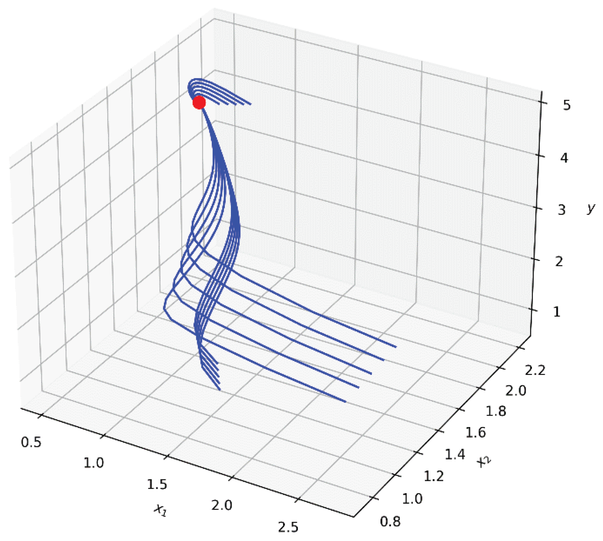
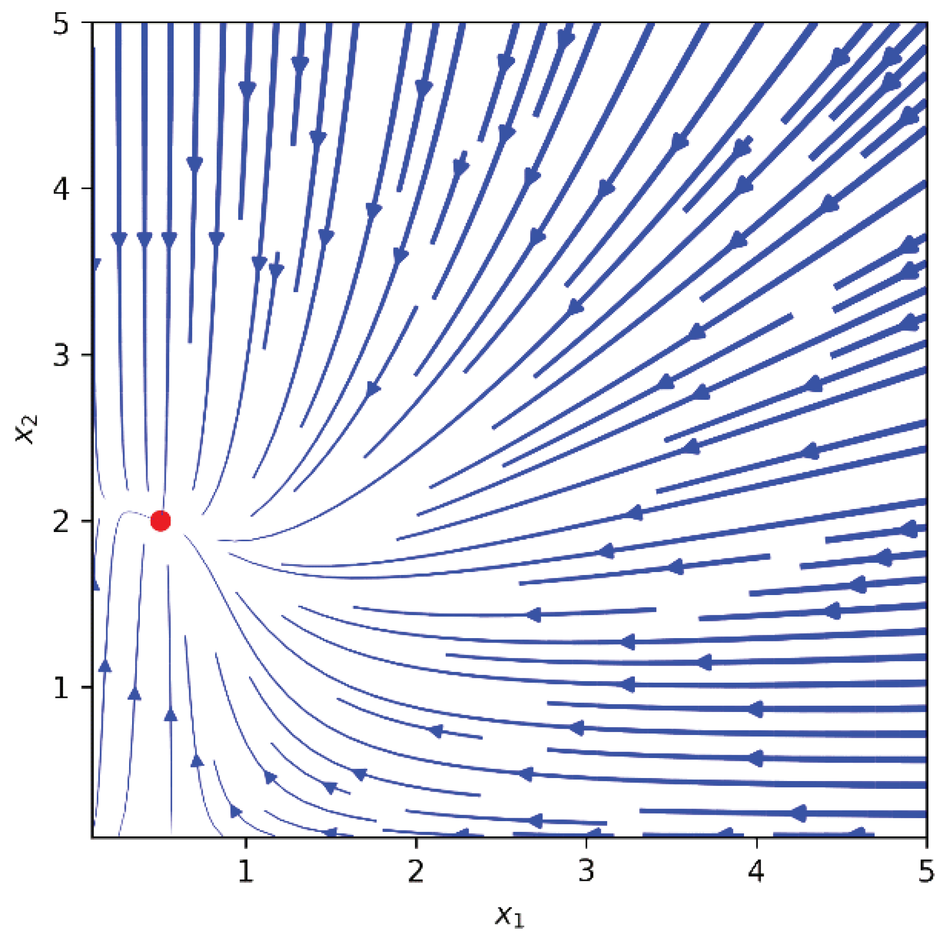
The phase portrait for the equilibrium state ${\overline{E}}_7(0.5,2,4)$ is shown in Figure 1. Projection onto the plane for the model (2), taking into account the selected set of parameters, is shown in Figure 2.

In Figure 1 and Figure 2, we marked the state of equilibrium ${\overline{E}}_7(0.5,2,4)$, corresponding to the selected set of parameters by the red dot. It should be highlighted that this equilibrium state is a stable node with permanent coexistence. It is possible to obtain another type of phase portrait with a stable state of equilibrium by changing the form of the criterion (3).

3. Deterministic Models with Control and Methods of Their Research

We formulate the optimal control problem for the population model (2). Let the differential equations of the controlled model have the form

$$\begin{array}{cc}\hfill {\dot{x}}_1& =x_1(a_1-{\epsilon }_{11}{x}_1-{\epsilon }_{12}{x}_2-by)-u_1,\hfill \\ \hfill {\dot{x}}_2& =x_2(a_2-{\epsilon }_{21}{x}_1-{\epsilon }_{22}{x}_2-by)-u_2,\hfill \\ \hfill \dot{y}& =y(-c+d{x}_1+d{x}_2)-u_3,\hfill \end{array}$$

(4)

where $u_i,i=1,2,3$ are control functions. Other designations are similar to the designations for the model (1). The initial and boundary conditions for the model (4) have the form

$$X\left(0\right)=(0,0,0),X\left(T\right)=(x_{11},x_{21},y_1),$$

(5)

$$0\le u_1\le u_{11},0\le u_2\le u_{21},0\le u_3\le u_{31},t\in [0,T].$$

(6)

For the Equations (4)–(6), we propose the following control quality functional:

$$J\left(U\right)={\int }_0^T∥U\left(t\right)∥dt,U=(u_1,u_2,u_3).$$

(7)

Note that minimization of functional (7) corresponds to minimization of losses from regulation of population density $x_1,x_2,y$. Thus, the optimal control problem for (4) is as follows: find such a $J\left(u\right)\to min$, that satisfies conditions (5), (6) taking into account $x_i>0,y>0,i=1,2$.

By analogy with the work [28] for the design of controls, we use a parametric control model in the form of polynomials. The specified model has the form

$$u_i\left(t\right)=∥R\mathsf{\Omega }∥,R={(r_{i1},r_{i2},\dots ,r_{in})}^{*},\mathsf{\Omega }=(t^0,t^1,\dots ,t^m),i=1,2,3.$$

Note that the control model parameters are the coefficients $r_{i1},r_{i2},\dots ,r_{in}$. We propose a method for calculating $r_{i1},r_{i2},\dots ,r_{in}$ using heuristic algorithms of global parametric optimization.

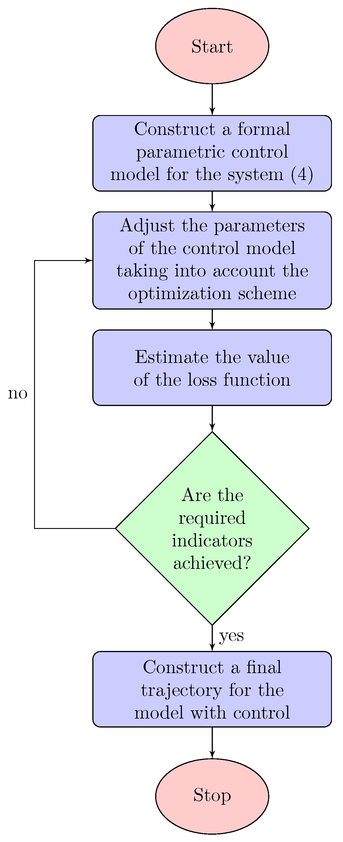
As it is possible to use various types of parametric control for (4), we propose a generalized algorithm for constructing optimal trajectories based on reinforcement learning. The block diagram of the algorithm is shown in the Figure 3.

Thus, the optimal control problem consists in finding such $u_i=u_i\left(t\right)$ that satisfy (5), (6), (7). To solve this problem using the algorithm in Figure 3 it is necessary to

(a)

construct the loss function,

(b)

construct a parametric control model and

(c)

use the global parametric optimization algorithm to find the coefficients of the control model with a minimum loss function.

We propose the design of stochastic models with control taking into account the “predator–two prey” interaction. To study such models, it is advisable to use the control laws $u_1$, $u_2$ and $u_3$ using the algorithm for obtaining the optimal trajectory of the model (4).

We use the algorithm in Figure 3 within the framework of solving the optimal control problem for the model (4) formulated in this article. Loss function to be minimized is

$$f\left(k_1[X\left(T_e\right)-X\left(T\right)],k_{2}J\left(U\right)\right),$$

(8)

where $k_1$, $k_2$ are weight coefficients, $X\left(T_e\right)$ is the value of $X\left(T\right)$ at step 4 of the algorithm in Figure 3, f is a scalar ranking function.

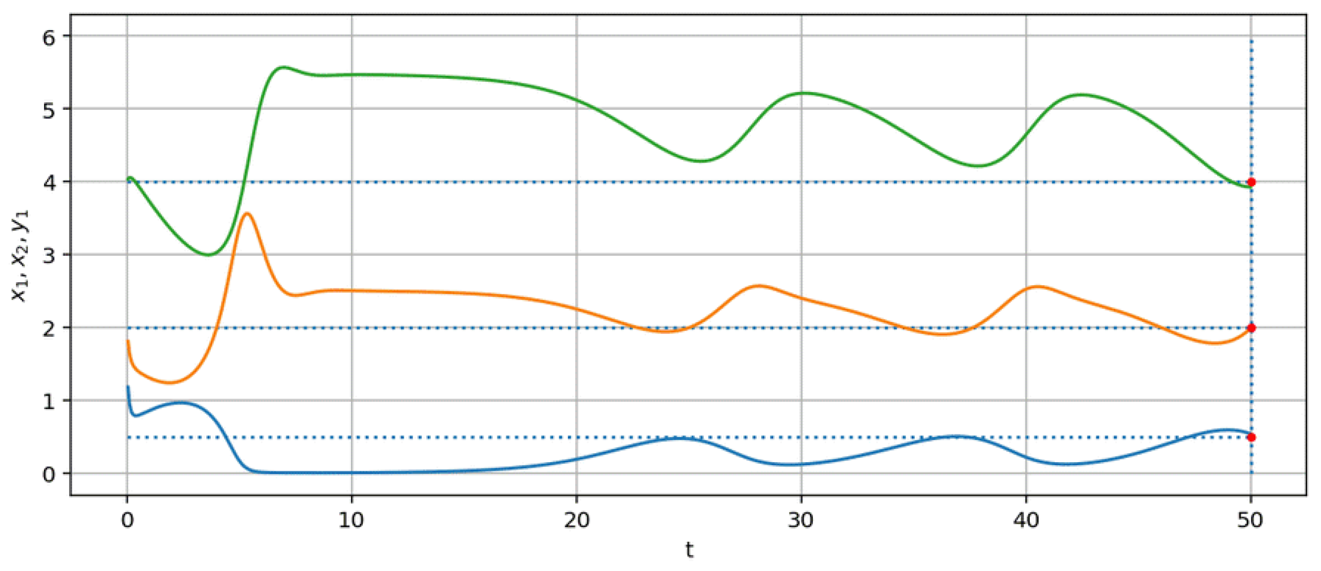
To find the coefficients of the matrix R and carry out computational experiments, a program in Python 3 is developed. The following values of the parametric coefficients with $\delta =(16,8,8,4,3.5,1,1,2.5/3,1/3)$ are obtained:

$$\left(\begin{array}{c}{R}_1\\ R_2\\ R_3\end{array}\right)=\left(\begin{array}{ccc}-8.6426\times {10}^{-3}& 8.8785\times {10}^{-4}& -1.0422\times {10}^{-5}\\ 9.1043\times {10}^{-2}& -7.1641\times {10}^{-3}& 1.4524\times {10}^{-4}\\ -1.8462\times {10}^{-2}& 3.8469\times {10}^{-3}& -8.4859\times {10}^{-5}\end{array}\right)$$

Small values of the parametric coefficients are consistent with the optimality criterion (7). The trajectories of the controlled system (4) with the coefficient matrix R are shown in Figure 4.

Note that at $t<20$ there is no oscillating change in population density in the controlled system. At $t>20$, the type of the motion becomes close to an uncontrollable system, while the trajectory satisfies the boundary conditions with respect to $X\left(T\right)$. Further, in Section 4, we carry out the stochastization of the models (2), (4) to study the qualitative features of the influence of the synthesized control law on the dynamics of population density.

4. Stochastization of the Trophic Chain Model

Consider a system of n components in which s different interactions occur:

$$\sum _a{N}_a^A{X}_a\stackrel{k_A^{+}}{\underset{k_A^{-}}{\rightleftarrows }}\sum _a{M}_a^A{X}_a,A=\overline{1,s},a=\overline{1,n}.$$

Coefficient $N_a^A$ at $X_a$ is a number of components of the form $X_a$ on the left part of the equation, $M_a^A$ is a number of components of the form $X_a$ on the right part of the equation. We use a vector representation:

$$\begin{array}{cc}\hfill & x=(x_1,x_2,\dots ,x_n),\hfill \\ \hfill & N^A=(N_1^A,N_2^A,\dots ,N_n^A),\hfill \\ \hfill & M^A=(M_1^A,M_2^A,\dots ,M_n^A),\hfill \end{array}$$

where $x_a$ is a number of components of the form $X_a$. We also define

$$r^A=M^A-N^A.$$

Thus, one step of interaction A in the forward and reverse directions can be written in the form of two relations:

$$\begin{array}{cc}\hfill & x\to x+r^A,\hfill \\ \hfill & x\to x-r^A.\hfill \end{array}$$

Probabilities of transition from the state x to state $x\pm r^A$ per unit of time are proportional to the number of ways of choosing the combination $N_a^A$ or $M_a^A$ from x components and are defined by the expressions

$$\begin{array}{cc}\hfill & s_A^{+}\left(x\right)=k_A^{+}\prod _a\frac{x_a!}{(x_a-N_a^A)!},\hfill \\ \hfill & s_A^{-}\left(x\right)=k_A^{-}\prod _a\frac{x_a!}{(x_a-M_a^A)!}.\hfill \end{array}$$

Thus, the general form of the master equation for an integer variable x varying in steps of length $r^A$ takes the form:

$$\begin{array}{c}{\partial }_{t}P(x,t)=\sum _A\left[\left(s_A^{-}(x+r^A)P(x+r^A,t)-s_A^{+}\left(x\right)P(x,t)\right)\right.+\hfill \\ \hspace{1em}\hspace{1em}\hspace{1em}\hspace{1em}\hspace{1em}\hspace{1em}\hspace{1em}\hspace{1em}\hspace{1em}\hspace{1em}\hspace{1em}\hspace{1em}\hspace{1em}\hspace{1em}\hspace{1em}\hspace{1em}\hspace{1em}\hspace{1em}+\left.\left(s_A^{+}(x-r^A)P(x-r^A,t)-s_A^{-}\left(x\right)P(x,t)\right)\right].\hfill \end{array}$$

(9)

Further, the Kramers–Moyal expansion is used to transition from the master equation to the Fokker–Planck equation. We consider the following assumptions. First, it is assumed that only small jumps take place, i.e., $s_A\left(x\right)$ is a function that changes slowly with x. The second assumption is that $P(x,t)$ also slowly changes with change x. Then, it is possible to perform a translation from the point $(x\pm r^A)$ to point x taking into account the decomposition of the right part into a Taylor series:

$${\partial }_{t}P(x,t)=\sum _A\left[\sum _j\left(\frac{{(r^A\nabla )}^j}{j!}{s}_A^{-}\left(x\right)P(x,t)\right)+\sum _j\left(\frac{{(-r^A\nabla )}^j}{j!}{s}_A^{+}\left(x\right)P(x,t)\right)\right].$$

Discarding terms of order higher than two, we obtain the Fokker–Planck equation

$${\partial }_{t}P(x,t)=-\sum _a{\partial }_a\left[F_a\left(x\right)P(x,t)\right]+\frac{1}{2}\sum _{a,b}{\partial }_a{\partial }_b\left[G_{ab}\left(x\right)P(x,t)\right],$$

(10)

where

$$\begin{array}{cc}\hfill & F_a\left(x\right)=\sum _A{r}_a^A\left[s_A^{+}\left(x\right)-s_A^{-}\left(x\right)\right],\hfill \\ \hfill & G_{ab}\left(x\right)=\sum _A{r}_a^A{r}_b^A\left[s_A^{+}\left(x\right)+s_A^{-}\left(x\right)\right].\hfill \end{array}$$

The Fokker–Planck equation describes the time evolution of the probability density function. For the Fokker–Planck Equation (10), one can write down the corresponding stochastic differential equation in the Langevin form

$$dx=f(x,t)dt+g(x,t)dW,$$

where $x\in R^N$ is the system state function, $W\in R^N$ is the standard N-dimensional Brownian motion. It is known that the following relations hold for the coefficients:

$$\begin{array}{cc}\hfill & f\left(x\right)=F\left(x\right),\hfill \\ \hfill & g\left(x\right)=G\left(x\right)G{\left(x\right)}^T.\hfill \end{array}$$

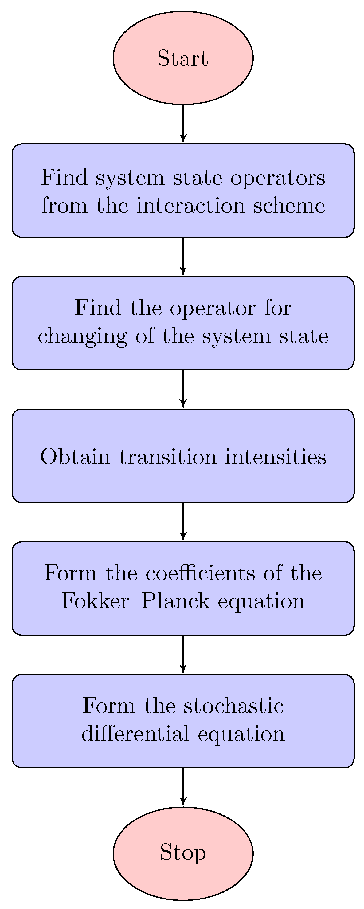
The algorithm aimed at practical application for obtaining a stochastic differential equation from the interaction scheme shown on Figure 5.

A numerical experiment is carried out for various sets of the model parameters [32]. It is found that for the particular case of the model (1) under the constraints ${\epsilon }_{11}={\epsilon }_{22}={\epsilon }_{12}={\epsilon }_{21}=\epsilon$ and $b_1=b_2$, $a_1=a_2$, $d_1=d_2$ the stability type of systems is significantly influenced by the coefficients of intraspecific and interspecific competition. Oscillations are formed if $\epsilon =\delta =0$ and if $a_1=k{a}_2$, $d_1=l{d}_2$ with $l=k$. At $\epsilon =\delta \ne 0$ the oscillations are damped. At $a_1=k{a}_2$, $d_1=l{d}_2$ with $l\ne k$ one of the populations of prey is dying out.

Next, we will consider the application of this method to the model (2). According to the method described above, for stochastization of the model it is necessary to write down the interaction scheme. Suppose that system interactions defined by the following scheme:

$$\begin{array}{cc}\hfill & X_i\stackrel{a_i}{\to }2X_i,i=1,2,\hfill \\ \hfill & X_i+X_j\stackrel{{\epsilon }_{ij}}{\to }{X}_j,i,j=1,2,\hfill \\ \hfill & X_i+Y\stackrel{d}{\to }2Y,X_i+Y\stackrel{b}{\to }Y,i=1,2,\hfill \\ \hfill & Y\stackrel{c}{\to }0.\hfill \end{array}$$

(11)

In (11), each line corresponds to a certain type of interaction between populations. Lines 1 and 4 define, respectively, natural reproduction and mortality of population species, provided that there are no other factors. Line 2 for $i=j$ describes intraspecific competition. The specified line for $i\ne j$ corresponds to interspecific competition. Line 3 defines a predator-prey relationship.

For the interaction scheme (11) of the model (2) using the developed software package the coefficients of the three-dimensional Fokker–Planck equation are obtained:

$$F\left(x\right)=\left(\begin{array}{c}{a}_1{x}_1-{\epsilon }_{11}{x}_1^2-{\epsilon }_{12}{x}_2{x}_1-by{x}_1\\ a_2{x}_2-{\epsilon }_{21}{x}_1{x}_2-{\epsilon }_{22}{x}_2^2-by{x}_2\\ -cy+d{x}_{1}y+d{x}_{2}y\end{array}\right),G\left(x\right)=\left(\begin{array}{ccc}{G}_{11}& 0& 0\\ 0& G_{22}& 0\\ 0& 0& G_{33}\end{array}\right),$$

where $F\left(x\right)$ is the drift vector, the $G\left(x\right)$ is the diffusion matrix, $G_{11}=a_1{x}_1+{\epsilon }_{11}{x}_1^2+{\epsilon }_{12}{x}_2{x}_1+by{x}_1$, $G_{22}=a_2{x}_2+{\epsilon }_{21}{x}_1{x}_2+{\epsilon }_{22}{x}_2^2+by{x}_2$, $G_{33}=cy+d{x}_{1}y+d{x}_{2}y$.

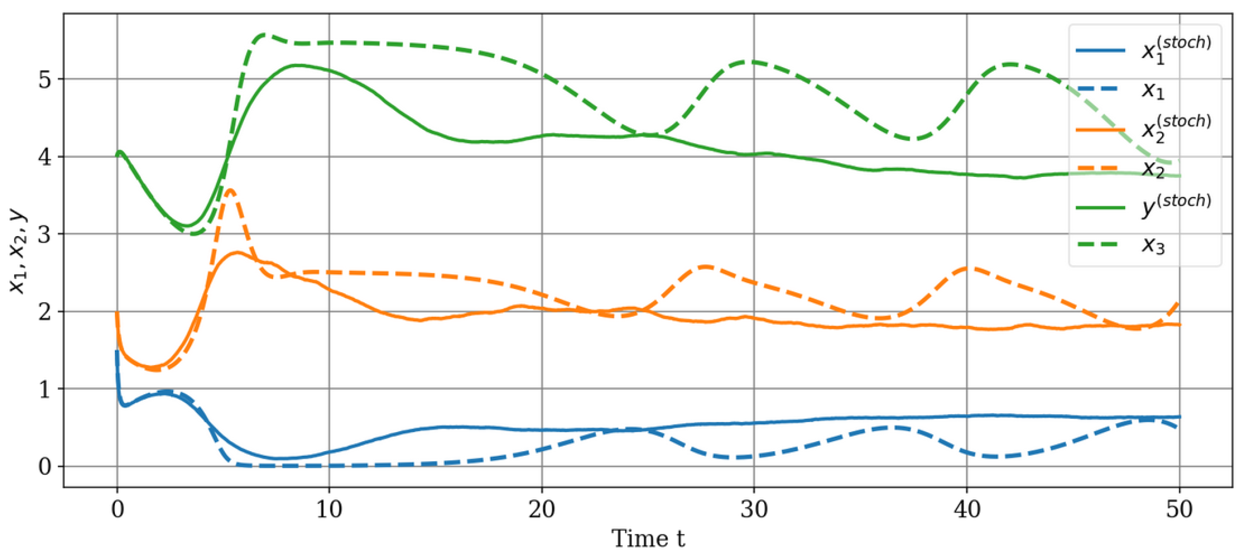
For the numerical analysis of the obtained stochastic model, we consider the time interval [0, 50]. The choice of parameters is consistent with the choice of parameters for the deterministic model (2). Figure 6 shows the trajectories of the stochastic model in comparison with the trajectories of the deterministic model (2).

The next step in the study of the model is the construction of a stochastic model for a system (4) with control. Similarly to a system without control we obtain the interaction scheme which will have the following form:

$$\begin{array}{cc}\hfill & X_i\stackrel{a_i}{\to }2X_i,i=1,2,\hfill \\ \hfill & X_i+X_j\stackrel{{\epsilon }_{ij}}{\to }{X}_j,i,j=1,2,\hfill \\ \hfill & X_i+Y\stackrel{d}{\to }2Y,X_i+Y\stackrel{b}{\to }Y,i=1,2,\hfill \\ \hfill & Y\stackrel{c}{\to }0,\hfill \\ \hfill & X_i\stackrel{u_i}{\to }0,Y\stackrel{u_3}{\to }0,i=1,2.\hfill \end{array}$$

(12)

The description of the top four lines (12) corresponds to the scheme (11), and the last line is added to describe the control.

For the interaction scheme (12) of the model (4), the coefficients of the three-dimensional Fokker–Planck equation are obtained:

$$F\left(x\right)=\left(\begin{array}{c}{a}_1{x}_1-{\epsilon }_{11}{x}_1^2-{\epsilon }_{12}{x}_2{x}_1-by{x}_1-u_1\\ a_2{x}_2-{\epsilon }_{21}{x}_1{x}_2-{\epsilon }_{22}{x}_2^2-by{x}_2-u_2\\ -cy+d{x}_{1}y+d{x}_{2}y-u_3\end{array}\right),G\left(x\right)=\left(\begin{array}{ccc}{G}_{11}& 0& 0\\ 0& G_{22}& 0\\ 0& 0& G_{33}\end{array}\right),$$

where $F\left(x\right)$ is the drift vector, the $G\left(x\right)$ is the diffusion matrix, $G_{11}=a_1{x}_1+{\epsilon }_{11}{x}_1^2+{\epsilon }_{12}{x}_2{x}_1+by{x}_1+u_1$, $G_{22}=a_2{x}_2+{\epsilon }_{21}{x}_1{x}_2+{\epsilon }_{22}{x}_2^2+by{x}_2+u_2$ and $G_{33}=cy+d{x}_{1}y+d{x}_{2}y+u_3$.

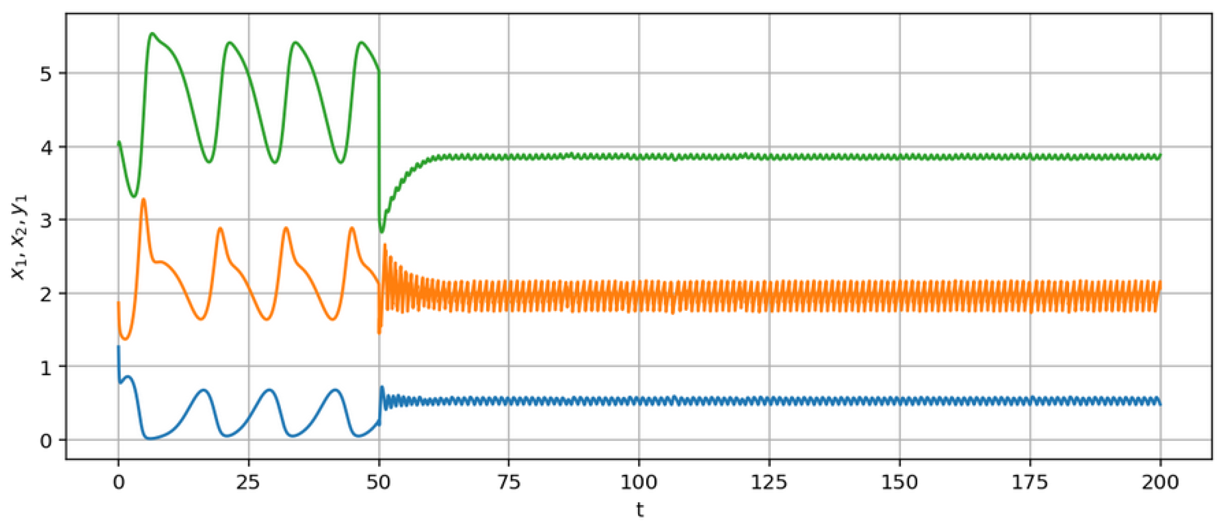
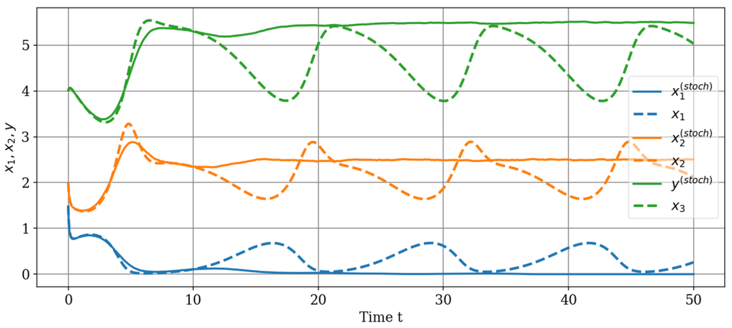
For a numerical experiment in relation to a system with control, parameters similar to the parameters of a system without control are chosen. The results of the numerical solution of the stochastic differential equation in comparison with the ordinary differential equation are presented in Figure 7.

A comparative analysis of the deterministic system (2) behavior and corresponding stochastic system behavior shows that for the system without control the stochastization destroys oscillatory trajectories. These trajectories acquire a monotonous character and enter a stationary mode, which is associated with the extinction of the $x_1$ population. In turn, the stochastization of the controlled system allows to keep such $x_1$ population density that does not vanish. It is worth nothing that the values $x_1,x_2,y$ at time 50 are close to the optimal values corresponding to the deterministic system (4).

5. Optimization of Deterministic Model Trajectories Using Artificial Neural Networks

Next, we consider the problem of optimizing the trajectories of a population model using an algorithm based on a neural network controller. We introduce an additional restriction on the control in the system (4). Let the control functions multiplicatively depend on the density of the corresponding population. Taking into account this restriction, the equations of the system take the form

$$\begin{array}{cc}\hfill {\dot{x}}_1& =x_1(a_1-{\epsilon }_{11}{x}_1-{\epsilon }_{12}{x}_2-by)-u_1{x}_1,\hfill \\ \hfill {\dot{x}}_2& =x_2(a_2-{\epsilon }_{21}{x}_1-{\epsilon }_{22}{x}_2-by)-u_2{x}_2,\hfill \\ \hfill \dot{y}& =y(-c+d{x}_1+d{x}_2)-u_{3}y.\hfill \end{array}$$

(13)

Notations of the model (13) are explained in Section 2. We consider a problem in the search for the optimal control law which is consistent with the asymptotic stability of the equilibrium state and with the permanent coexistence of two prey and a predator.

We propose controller based on an artificial neural network the topology of which is shown in Figure 8.

The loss value is applied to the inputs $(e_1,e_2,e_3)$, the loss value with delay is applied to the inputs $({\widehat{e}}_1,{\widehat{e}}_2,{\widehat{e}}_3)$. Two hidden layers of the neural network have a tangential activation function, the output layer has a logistic activation function with a fixed multiplier. The neural network is trained according to the algorithm in Figure 3, and the loss function has the form (8).

To train a neural network and perform computational experiments, software is developed by the aid of Python 3. The original implementation of the neural network computing module on the basis of Numpy mathematical package is used. We consider the activation of neural network control at $t>50$. Training is carried out for equilibrium state ${\overline{E}}_7(0.5,2,4)$. The trajectories of the system (13) at $\delta =(16,8,8,4,3.5,1,1,2.5/3,1/3)$ are shown in Figure 9.

Note that upon activation of neural network control, the system (13) comes to a state of equilibrium that is close to ${\overline{E}}_7(0.5,2,4)$. Oscillations are observed with a small period and amplitude, and the oscillations do not damp with an increase in the control frequency.

6. Discussion

The carried out qualitative and quantitative analysis of the models of population dynamics and the obtained analytical results make it possible to construct the regions of stability and permanent coexistence of species for various special cases of the model (1). Figure 1 and Figure 2 show the phase portraits for such a set of parameters, which is obtained using evolutionary calculations. At the same time, evolutionary calculations make it possible to search for equilibrium states belonging to the regions of stability and permanent coexistence. The carried out computational experiments show the conformity of the numerical results and Theorems 1–6.

The proposed formulation of the optimal control problem for the model (4) is new and provides for both the possibility of phase and mixed constraints and the use of parametric control, in particular, polynomial control. The novelty of the approach to the synthesis of the model (4) controllers lies in the use of adapted machine learning algorithms based on differential evolution. The considered control quality criterion is aimed at unconditional minimization of the impact on populations. The synthesized control satisfies the conditions of stability and permanent coexistence, taking into account the optimality and the given boundary conditions (Figure 4). The prospect of further research is to consider other type of control quality criteria associated with the control of individual populations.

The transition from models defined by vector ordinary differential equations to the corresponding stochastic models makes it possible to identify and compare qualitative features of dynamics. For uncontrolled and controlled cases, interaction schemes (11) and (12) are constructed, and the influence of stochastization on the dynamics of population density in a model with trophic chains is studied (Figure 6 and Figure 7). Comparative analysis showed that for an uncontrolled system, stochastization leads to the degeneration of the oscillatory mode of trajectories into a monotonic one with the extinction of prey population (Figure 6). The results of stochastization of the controlled system showed that the densities of all three populations remain positive and correlate with the deterministic system at $t=50$ (Figure 7).

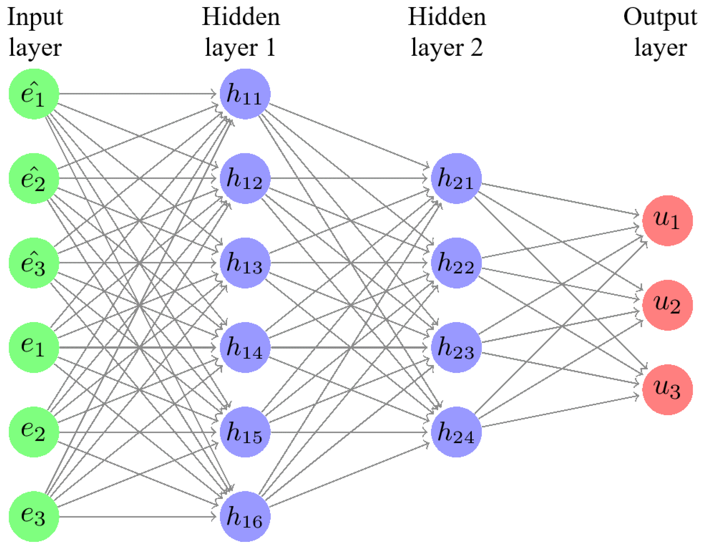
The proposed neural network approach to optimizing the trajectory dynamics of a population model makes it possible to study the features of constructing such a control that is multiplicatively depend on the population density. On the basis of the developed topology of the neural network (Figure 8), a controller is proposed, the implementation of which gives trajectories with the properties of asymptotic stability (Figure 9).

The instrumental and methodological support of mathematical modeling of population systems presented in Section 2, Section 3, Section 4 and Section 5 allows for a comprehensive study of the models under consideration.

Note that the proposed computational procedures involving intelligent analysis demonstrate a fairly high efficiency in solving problems of mathematical modeling of population systems. At the stage of studying deterministic models, the author’s software complex for modeling population systems based on artificial intelligence is used. The specified software package is developed in Python 3 using the mathematical libraries NumPy, SciPy and Matplotlib. As a tool for stochastization of the proposed models, a specialized software package is used to construct stochastic dynamic models and search for appropriate trajectories.

7. Conclusions

This paper proposes a new approach to the synthesis and analysis of nonlinear three-dimensional models of the population size dynamics taking into account trophic chains and competition in prey populations. For different sets of parameters, trajectories and corresponding phase portraits are constructed. The results of an analytical study of stability and permanent coexistence conditions are verified using computational experiments. For a positive equilibrium state for a given set of model parameters, it is shown that the considered equilibrium state belongs to the regions of stability and permanent coexistence of species. The conformity of theoretical results with the results of computational experiments is verified. Stochastization of the deterministic model for uncontrolled and controllable cases is carried out. Comparative analysis of deterministic and stochastic models shows that the behavior of models with the same sets of parameters may have significant differences.

The formulation of the optimal control problem using a parametric polynomial model is proposed. A generalized algorithm for optimal control based on the reinforcement learning is developed. A method for optimizing the trajectory dynamics of a population model on the basis of artificial neural networks using is proposed.

The applied significance of the paper’s results is due to the fact that models (2), (4) and their stochastic generalizations can serve to study the qualitative properties of not only ecological systems, but also socio-economic, demographic, chemical and physical systems. The obtained results can be used in solving problems such as modeling of deterministic and stochastic systems, optimal control of populations and resources, predicting the behavior of dynamic systems in the presence of noise, formalized description of technological processes. In addition, the results can be used in the development of algorithmic support for problem-oriented software packages, as well as in solving of reinforcement learning problems.

Prospects for further research are in the synthesis and computer study of population models with partial control and in expanding the range of numerical methods of global parametric optimization in the search for optimal trajectories. In addition, a promising area of research is the study of the influence of stochastization on the nonlinear models dynamics with neural network control.