Analysis of a Discrete-Time Queueing Model with Disasters

Abstract

Queueing models with disasters can be used to evaluate the impact of a breakdown or a system reset in a service facility. In this paper, we consider a discrete-time single-server queueing system with general independent arrivals and general independent service times and we study the effect of the occurrence of disasters on the queueing behavior. Disasters occur independently from time slot to time slot according to a Bernoulli process and result in the simultaneous removal of all customers from the queueing system. General probability distributions are allowed for both the number of customer arrivals during a slot and the length of the service time of a customer (expressed in slots). Using a two-dimensional Markovian state description of the system, we obtain expressions for the probability, generating functions, the mean values, variances and tail probabilities of both the system content and the sojourn time of an arbitrary customer under a first-come-first-served policy. The customer loss probability due to a disaster occurrence is derived as well. Some numerical illustrations are given.

1. Introduction

Queueing models with negative arrivals have been studied extensively over the last decades, owing to their applicability in the performance analysis of a wide range of systems, such as computers, telecommunication systems and manufacturing systems. The basic version of such models, known as the G-queue, is due to Gelenbe [1] and considers the notion of a negative customer that, upon arrival, removes one ordinary (or positive) customer from the queueing system according to some killing strategy, such as the removal of the customer in service or the removal of the customer that arrived most recently, if any. Another type of negative arrival, introduced by Towsley and Tripathi [2], is disasters that upon occurrence result in the simultaneous removal of all customers from the queueing system. As such, queueing models with disasters can be used to evaluate the impact of a machine breakdown in a production system, a system reset in a service facility or a virus infection affecting a computer system. Queues with disasters are also referred to in the literature as queues with mass exodus, catastrophes, queue flushing or stochastic clearing [3].

In this paper, our focus is on queueing models with disasters in the discrete-time domain, which have so far been analyzed to a lesser extent than their continuous-time counterparts. The first study [3] on discrete-time queues with disasters considered the Geo/Geo/1 queueing model with a Bernoulli distribution of the number of customer arrivals per slot and geometric service times under the impact of Bernoulli disasters. A similar disaster model was used in [4] to model the behavior of an email contact center. A transient analysis of the system content in the Geo/Geo/1 disaster model was performed in [5]. The extension to a discrete-time Geo/G/1 disaster model with Bernoulli arrivals and general independent service times was considered in [6] (system content) and [7,8] (sojourn time). The Geo/G/1 disaster model was also analyzed in [9] under an N-policy operation and in [10,11,12] under repair times after a disaster. The queue length and sojourn time in a G/Geo/1 disaster queue with general independent interarrival times between customers and, at most, 1 customer arrival per slot were investigated in [13], while disaster queues with bursty Bernoulli arrivals and geometric service times were considered in [14,15].

Our current work further extends the existing results in the literature to a discrete-time disaster model, where general probability distributions are allowed for both the number of customer arrivals during a slot and the length of a customer service time. We present a full queueing analysis of this queueing model with disasters and derive expressions for the probability generating functions as well as the mean values, variances and tail probabilities of both the system content and the sojourn time under a first-come-first-served (FCFS) policy.

For related work on discrete-time G-queues with negative customers, the reader is referred to [3,7,14,16,17,18,19,20,21,22,23]. For work on continuous-time queueing models with negative customers and/or disasters, we refer to the bibliography in [24,25] and the more recent papers [26,27,28,29,30,31,32,33,34,35,36]. Additionally, somewhat related to this paper in the sense that customers may leave the system before their service is completed are queueing models with customer impatience or deadlines; we refer to [37] and the references therein for an overview of such models.

The paper is organized as follows. The specific assumptions of the considered queueing model are detailed in Section 2. In Section 3, system equations are established that describe the evolution of the state of the queueing system from slot to slot. Based on these system equations, an expression for the steady-state joint probability generating function (pgf) of the system state variables is obtained in Section 4 in terms of the unknown probability of having an empty system. A technique to calculate this remaining unknown is presented in Section 5, together with the analysis of the main characteristics of the system content. Section 6 then derives the pgf of the unfinished work in the system, as an intermediate step for the analysis of the characteristics of the sojourn time in Section 7. The customer loss probability due to a disaster occurrence is derived in Section 8. Some numerical examples to illustrate the analysis are given in Section 9, before the paper is concluded in Section 10.

2. Queueing Model

We consider a discrete-time queueing system with one server and an infinite waiting room for customers. The time axis is divided into fixed-length slots. New customers arrive at the system in a stochastic way, according to a general independent arrival process, i.e., the numbers of customers arriving during the consecutive slots are assumed to be independent and identically distributed (i.i.d.) discrete random variables. Their common probability mass function (pmf) is indicated as

$$a\left(n\right)=\mathrm{Prob}\left[n\mathrm{customer}\mathrm{arrivals}\mathrm{during}\mathrm{a}\mathrm{slot}\right],n\ge 0,$$

with corresponding pgf

$$A\left(z\right)=\sum _{n=0}^{\infty }a\left(n\right)z^n.$$

The mean arrival rate, i.e., the mean number of customer arrivals during a slot, is given by

$$\lambda =A^{\prime }\left(1\right).$$

The service of a customer is assumed to require a positive integer number of slots and can start or end at slot boundaries only. More specifically, the service times of the customers are assumed to constitute a sequence of i.i.d. positive discrete random variables with common pmf

$$s\left(n\right)=\mathrm{Prob}\left[\mathrm{service}\mathrm{of}\mathrm{a}\mathrm{customer}\mathrm{takes}n\mathrm{slots}\right],n\ge 1,$$

corresponding pgf

$$S\left(z\right)=\sum _{n=1}^{\infty }s\left(n\right)z^n$$

and mean service time

$$S^{\prime }\left(1\right)=\frac{1}{\mu },$$

where $\mu$ is the so-called mean service rate, i.e., the mean number of customers that can be served per slot. The service times are also assumed to be independent of the random variables used in the description of the arrival process.

The queueing system is subject to so-called independent Bernoulli disasters, i.e., during any slot, either a disaster occurs with probability $\sigma$ ($\sigma >0$) or no disaster occurs with probability $1-\sigma$, independently from slot to slot. When such a disaster occurs during a slot, all customers in the system as well as all new arrivals during the slot get lost. In the sequel, we specifically consider that in case of a disaster, all customers are removed from the system at the end of the disaster slot, thus leaving the system empty at the end of that slot.

3. System Equations

Let the random variable $u_k$ denote the system content, i.e., the total number of customers in the system, at the beginning of slot k. Let $a_k$ be the number of customer arrivals during slot k, and let $d_k$ indicate the number of disasters occurring during slot k. Clearly, to describe the evolution of the system content from slot k to slot $k+1$, some information is also needed about the still remaining part of the service time of the customer in service, if any, at the beginning of slot k. We therefore define the random variable $h_k$ as follows: $h_k$ denotes the remaining number of slots needed to complete the service of the customer currently in service at the beginning of slot k, if $u_k\ge 1$, and $h_k=0$ if $u_k=0$. Note that this definition implies that $h_k>0$ if and only if $u_k>0$. Similarly, $h_k=0$ if and only if $u_k=0$. Finally, we let $s^{*}$ indicate the service time of the next customer to receive service at the beginning of slot k.

With these definitions, the behavior of the queueing system is then characterized by the following system equations:

(a)

If $d_k=1$:

$$h_{k+1}=u_{k+1}=0.$$

(1)

(b)

If $d_k=0$ and $h_k=0$:

$$\begin{array}{cc}\hfill & u_{k+1}=a_k,\hfill \end{array}$$

(2)

$$\begin{array}{cc}\hfill & h_{k+1}=\left\{\begin{array}{cc}0 , \hfill & \mathrm{if} a_k=0,\hfill \\ s^{*} , \hfill & \mathrm{if} a_k>0.\hfill \end{array}\right.\hfill \end{array}$$

(3)

(c)

If $d_k=0$ and $h_k=1$:

$$\begin{array}{cc}\hfill & u_{k+1}=u_k-1+a_k,\hfill \end{array}$$

(4)

$$\begin{array}{cc}\hfill & h_{k+1}=\left\{\begin{array}{cc}0 , \hfill & \mathrm{if} u_k=1\mathrm{and}{a}_k=0,\hfill \\ s^{*} , \hfill & \mathrm{if} u_k-1+a_k>0.\hfill \end{array}\right.\hfill \end{array}$$

(5)

(d)

If $d_k=0$ and $h_k>1$:

$$\begin{array}{cc}\hfill & u_{k+1}=u_k+a_k,\hfill \end{array}$$

(6)

$$\begin{array}{cc}\hfill & h_{k+1}=h_k-1.\hfill \end{array}$$

(7)

Equations (1)–(7) are based on the following observations. If there is a disaster in slot k, all customers (including new arrivals during slot k) are removed from the system, so we have an empty system at the beginning of slot $k+1$. In case no disaster occurs during slot k and the system is empty at the beginning of slot k, then at the beginning of slot $k+1$, the system only contains the new arrivals during slot k, and, if any, one of these new arrivals are taken into service. If $h_k=1$ and there is no disaster in slot k, the customer in service leaves the system at the end of slot k; moreover, the service of a new customer starts at the beginning of slot $k+1$ unless the system has become empty. Finally, if $h_k>1$ and there is no disaster in slot k, no customer leaves the system at the end of slot k, and the remaining service time of the customer in service decreases by one slot.

It is obvious from the system equations that knowledge of the values of $h_k$ and $u_k$ suffices to determine the joint probability distribution of $h_{k+1}$ and $u_{k+1}$. The sequence of pairs $\left\{(h_k,u_k)\right\}$, therefore, forms a two-dimensional first-order Markov chain and the state of the queueing system in slot k is fully characterized by the pair $(h_k,u_k)$.

4. Queueing Analysis

By means of the system Equations (1)–(7), we can now analyze the queueing behavior. To do so, we first define $P_k(x,z)$ as the joint pgf of the state vector $(h_k,u_k)$ at the beginning of slot k:

$$P_k(x,z)\triangleq \mathrm{E}\left[x^{h_k}{z}^{u_k}\right]=\sum _{i=0}^{\infty }\sum _{n=0}^{\infty }\mathrm{Prob}\left[h_k=i,u_k=n\right]x^i{z}^n,$$

where the operator $\mathrm{E}\left[\dots \right]$ indicates the expected value of the random expression between the square brackets.

The next step in our analysis is then to derive a relationship between the pgfs $P_k(x,z)$ and $P_{k+1}(x,z)$ of the state vectors at the beginning of two consecutive slots. Using Equations (1)–(7), we write the function $P_{k+1}(x,z)$ as

$$\begin{array}{cc}\hfill P_{k+1}(x,z)& \triangleq \mathrm{E}\left[x^{h_{k+1}}{z}^{u_{k+1}}\right]\hfill \\ \hfill & =\mathrm{Prob}\left[d_k=1\right]\mathrm{E}\left[x^0{z}^0|d_k=1\right]\hfill \\ \hfill & +\mathrm{Prob}\left[h_k=0,a_k=0,d_k=0\right]\mathrm{E}\left[x^0{z}^0|h_k=0,a_k=0,d_k=0\right]\hfill \\ \hfill & +\mathrm{Prob}\left[h_k=0,a_k>0,d_k=0\right]\mathrm{E}\left[x^{s^{*}}{z}^{a_k}|h_k=0,a_k>0,d_k=0\right]\hfill \\ \hfill & +\mathrm{Prob}\left[h_k=1,u_k=1,a_k=0,d_k=0\right]\hfill \\ \hfill & ·\mathrm{E}\left[x^0{z}^0|h_k=1,u_k=1,a_k=0,d_k=0\right]\hfill \\ \hfill & +\mathrm{Prob}\left[h_k=1,u_k-1+a_k>0,d_k=0\right]\hfill \\ \hfill & ·\mathrm{E}\left[x^{s^{*}}{z}^{u_k-1+a_k}|h_k=1,u_k-1+a_k>0,d_k=0\right]\hfill \\ \hfill & +\mathrm{Prob}\left[h_k>1,d_k=0\right]\mathrm{E}\left[x^{h_k-1}{z}^{u_k+a_k}|h_k>1,d_k=0\right].\hfill \end{array}$$

(8)

Note that the system state variables $h_k$ and $u_k$ are statistically independent of the variables $a_k$, $d_k$ and $s^{*}$ due to the uncorrelated nature of both the customer arrival process and the occurrence of disasters from slot to slot and the i.i.d. nature of the service times of the customers. This allows us to further rewrite $P_{k+1}(x,z)$ as follows:

$$\begin{array}{cc}\hfill P_{k+1}(x,z)& =\mathrm{Prob}\left[d_k=1\right]+\mathrm{Prob}\left[d_k=0\right]\{\mathrm{Prob}\left[h_k=0\right]\mathrm{Prob}\left[a_k=0\right]\hfill \\ \hfill & +\mathrm{Prob}\left[h_k=0\right]\mathrm{Prob}\left[a_k>0\right]S\left(x\right)\mathrm{E}\left[z^{a_k}|a_k>0\right]\hfill \\ \hfill & +\mathrm{Prob}\left[h_k=1,u_k=1\right]\mathrm{Prob}\left[a_k=0\right]\hfill \\ \hfill & +\mathrm{Prob}\left[h_k=1,u_k-1+a_k>0\right]S\left(x\right)\mathrm{E}\left[z^{u_k-1+a_k}|h_k=1,u_k-1+a_k>0\right]\hfill \\ \hfill & +\mathrm{Prob}\left[h_k>1\right]\frac{1}{x}A\left(z\right)\mathrm{E}\left[x^{h_k}{z}^{u_k}|h_k>1\right]\}.\hfill \end{array}$$

(9)

Using the property that $\mathrm{Prob}\left[h_k=0\right]=P_k(0,0)$ and the law of total expectation, we then obtain

$$\begin{array}{cc}\hfill P_{k+1}(x,z)& =\sigma +(1-\sigma )\{P_k(0,0)A\left(0\right)+P_k(0,0)S\left(x\right)[A\left(z\right)-A\left(0\right)]\hfill \\ \hfill & +\mathrm{Prob}\left[h_k=1,u_k=1\right]A\left(0\right)\hfill \\ \hfill & +S\left(x\right)\{\mathrm{Prob}\left[h_k=1\right]\mathrm{E}\left[z^{u_k-1+a_k}|h_k=1\right]\hfill \\ \hfill & -\mathrm{Prob}\left[h_k=1,u_k=1\right]\mathrm{Prob}\left[a_k=0\right]\mathrm{E}\left[z^{u_k-1+a_k}|h_k=1,u_k=1,a_k=0\right]\}\hfill \\ \hfill & +\frac{1}{x}A\left(z\right)\{P_k(x,z)-\mathrm{Prob}\left[h_k=1\right]\mathrm{E}\left[x^{h_k}{z}^{u_k}|h_k=1\right]\hfill \\ \hfill & -\mathrm{Prob}\left[h_k=0\right]\mathrm{E}\left[x^{h_k}{z}^{u_k}|h_k=0\right]\left\}\right\}.\hfill \end{array}$$

(10)

Let us now define the function $R_k\left(z\right)$ as

$$R_k\left(z\right)\triangleq \mathrm{Prob}\left[h_k=1\right]\mathrm{E}\left[z^{u_k-1}|h_k=1\right]=\sum _{n=1}^{\infty }\mathrm{Prob}\left[h_k=1,u_k=n\right]z^{n-1},$$

(11)

such that $R_k\left(0\right)=\mathrm{Prob}\left[h_k=1,u_k=1\right]$. Then we finally find the following relationship between $P_k(x,z)$ and $P_{k+1}(x,z)$:

$$\begin{array}{cc}\hfill P_{k+1}(x,z)& =\sigma +(1-\sigma )\{P_k(0,0)A\left(0\right)[1-S\left(x\right)]+P_k(0,0)S\left(x\right)A\left(z\right)\hfill \\ \hfill & +R_k\left(0\right)A\left(0\right)+S\left(x\right)A\left(z\right)R_k\left(z\right)-S\left(x\right)A\left(0\right)R_k\left(0\right)\hfill \\ \hfill & +\frac{1}{x}A\left(z\right)\left\{P_k(x,z)-xz{R}_k\left(z\right)-P_k(0,0)\right\}\}.\hfill \end{array}$$

(12)

Since we are interested in the steady-state behavior of the queueing system, we let the time index k go to ∞. In steady state (for $k\to \infty$), the pgfs $P_k(x,z)$ and $P_{k+1}(x,z)$ both converge to a common limiting function

$$P(x,z)\triangleq \underset{k\to \infty }{\lim }{P}_k(x,z).$$

(13)

Note that due to the possible occurrence of disasters ($\sigma >0$), such a steady state will always exist. Equation (12) then leads to a linear equation for $P(x,z)$ with the following solution:

$$\begin{array}{cc}\hfill P(x,z)& =\frac{1}{x-(1-\sigma )A\left(z\right)}\{\sigma x+A\left(0\right)x(1-\sigma )[1-S(x\left)\right]\left[P\right(0,0)+R(0\left)\right]\hfill \\ \hfill & +P(0,0)A\left(z\right)(1-\sigma )\left[xS\right(x)-1]+A\left(z\right)x(1-\sigma )R\left(z\right)\left[S\right(x)-z]\},\hfill \end{array}$$

(14)

where

$$R\left(z\right)\triangleq \underset{k\to \infty }{\lim }{R}_k\left(z\right).$$

It now remains to determine the unknown function $R\left(z\right)$ and the two unknown probabilities $R\left(0\right)$ and $P(0,0)$. This can be done as follows. First note that, due to the fact that $h_k=0$ if and only if $u_k=0$, the following property holds:

$$P(x,0)=P(0,0),\mathrm{for}\mathrm{all}x.$$

In particular, this means that $P(1,0)$ as obtained from (14) should equal $P(0,0)$, which leads to the following relationship between $P(0,0)$ and $R\left(0\right)$:

$$P(0,0)=\sigma +A\left(0\right)(1-\sigma )\left[P\right(0,0)+R(0\left)\right].$$

(15)

Next, we notice that the pgf $P(x,z)$ must be bounded for all values of its arguments x and z such that $\left|x\right|\le 1$ and $\left|z\right|\le 1$. In particular, this should be true for $x=(1-\sigma )A\left(z\right)$ and $\left|z\right|\le 1$, since $(1-\sigma )\left|A\left(z\right)\right|\le 1$ for all such z, as $A\left(z\right)$ is a pgf. If we now choose $x=(1-\sigma )A\left(z\right)$ in Equation (14), where $\left|z\right|\le 1$, it is clear that the denominator of $P(x,z)$ vanishes. Of course, the numerator of $P(x,z)$ in (14) must then also be equal to zero for $x=(1-\sigma )A\left(z\right)$ with $\left|z\right|\le 1$. This requirement together with the relation (15) then leads to the following equation for $R\left(z\right)$:

$$(1-\sigma )A\left(z\right)R\left(z\right)=S\left((1-\sigma )A\left(z\right)\right)\frac{P(0,0)\left[\right(1-\sigma \left)A\right(z)-1]+\sigma }{z-S\left(\right(1-\sigma \left)A\right(z\left)\right)}.$$

(16)

From (14) together with Equations (15) and (16), an expression for $P(x,z)$ can then be derived in terms of the single unknown probability $P(0,0)$:

$$\begin{array}{cc}\hfill P(x,z)& =\frac{1}{x-(1-\sigma )A\left(z\right)}\{\sigma x+x[1-S(x\left)\right]\left[P\right(0,0)-\sigma ]\hfill \\ \hfill & +P(0,0)A\left(z\right)(1-\sigma )\left[xS\right(x)-1]\hfill \\ \hfill & +xS\left((1-\sigma )A\left(z\right)\right)\frac{P(0,0)\left[\right(1-\sigma \left)A\right(z)-1]+\sigma }{z-S\left(\right(1-\sigma \left)A\right(z\left)\right)}[S\left(x\right)-z]\}.\hfill \end{array}$$

(17)

The classical approach to determine the final remaining unknown $P(0,0)$ would now be to express the normalization condition for the joint distribution of the state vector. However, in our case it turns out that $P(1,1)=1$, irrespective of the value of $P(0,0)$. So, a different approach is needed to obtain $P(0,0)$, which is presented in the next section. Once $P(0,0)$ is determined and, hence, the joint probability generating function $P(x,z)$ is fully known, all main performance measures of the queueing system (namely the moments and tail probabilities of the system content and the sojourn time as well as the customer loss probability) can be derived directly from the function $P(x,z)$, i.e., without any need for inversion of this joint pgf or calculation of joint probabilities. The methodology is explained in the next sections.

5. System Content

The pgf $U\left(z\right)$ of the system content u observed at the beginning of a random slot in the steady state can be obtained from $P(x,z)$ by simply putting $x=1$: $U\left(z\right)=P(1,z)$. After rearranging some terms, we obtain

$$U\left(z\right)=\frac{S\left(\right(1-\sigma \left)A\right(z\left)\right)[1-(1-\sigma \left)A\right(z\left)\right](z-1)P(0,0)+\sigma z[1-S((1-\sigma )A\left(z\right)\left)\right]}{[1-(1-\sigma \left)A\right(z\left)\right][z-S((1-\sigma )A\left(z\right)\left)\right]}.$$

(18)

We can now find the unknown $P(0,0)=U\left(0\right)$ by noting that the function $U\left(z\right)$, as a pgf, must be bounded for all z with $\left|z\right|\le 1$. Using Rouché’s theorem, it can be shown (see Appendix A, Property A1) that the factor $z-S\left(\right(1-\sigma \left)A\right(z\left)\right)$ in the denominator of $U\left(z\right)$ in (18) has exactly one zero inside the unit circle in the complex z-plane. Let us denote this zero by $z^{*}$. It satisfies the following equation:

$$z^{*}-S\left((1-\sigma )A\left(z^{*}\right)\right)=0,\mathrm{with}\left|z^{*}\right|<1.$$

(19)

Clearly, the zero $z^{*}$ of the denominator must then also be a zero of the numerator of $U\left(z\right)$. This property then yields the following linear equation for $P(0,0)$:

$$z^{*}[1-(1-\sigma )A\left(z^{*}\right)](z^{*}-1)P(0,0)+\sigma z^{*}(1-z^{*})=0,$$

(20)

where we also use Equation (19). Since $z^{*}\ne 1$ and under the assumption that $z^{*}\ne 0$, the probability $P(0,0)$ then directly follows from (20) as

$$P(0,0)=\frac{\sigma }{1-(1-\sigma )A\left(z^{*}\right)}.$$

(21)

It is worth noting here that in view of (19), $z^{*}=0$ is only possible in the case that $A\left(0\right)=0$. In such a case, new arrivals occur in each slot and the system can only be empty at the beginning of a slot if there is a disaster during the previous slot, so $P(0,0)=\sigma$. The latter is, in fact, in full agreement with the result (21), so the expression (21) for $P(0,0)$ turns out to be generally valid. The value of $z^{*}$ in this expression for $P(0,0)$ needs to be determined numerically from (19), e.g., by means of Newton–Raphson’s method.

Based on the pgf $U\left(z\right)$, the moments and tail probabilities of the system content can now be derived, as explained below.

5.1. Mean and Variance of the System Content

In general, any moment of the system-content distribution can be obtained by expressing the desired moment of u as a function of the consecutive derivatives of the pgf $U\left(z\right)$ with respect to z for $z=1$. Here, we give the results obtained from Equation (18) for the mean value $\mathrm{E}\left[u\right]$ and the variance $\mathrm{var}\left[u\right]$ of the system content:

$$\mathrm{E}\left[u\right]=U^{\prime }\left(1\right)=\frac{1-\sigma }{\sigma }{A}^{\prime }\left(1\right)+\frac{S(1-\sigma )}{1-S(1-\sigma )}[P(0,0)-1]$$

(22)

and

$$\begin{array}{cc}\hfill \mathrm{var}\left[u\right]& =U^{″}\left(1\right)+U^{\prime }\left(1\right)-{U^{\prime }\left(1\right)}^2\hfill \\ \hfill & =\frac{1-\sigma }{\sigma }\left\{A^{\prime }\left(1\right)+A^{″}\left(1\right)+2{\left(A^{\prime }\left(1\right)\right)}^2\frac{1-\sigma }{\sigma }\right\}-\frac{2(1-\sigma )A^{\prime }\left(1\right)S(1-\sigma )}{\sigma (1-S(1-\sigma \left)\right)}\hfill \\ \hfill & +\frac{P(0,0)-1}{{[1-S(1-\sigma \left)\right]}^2}\left\{2(1-\sigma )A^{\prime }\left(1\right)S^{\prime }(1-\sigma )-S(1-\sigma )[1+S(1-\sigma )]\right\}\hfill \\ \hfill & -{\left\{\frac{1-\sigma }{\sigma }{A}^{\prime }\left(1\right)+\frac{S(1-\sigma )}{1-S(1-\sigma )}[P(0,0)-1]\right\}}^2.\hfill \end{array}$$

(23)

5.2. Tail Distribution of the System Content

Another important characteristic is the tail distribution of the system content. We use here an approximation technique as described, for example, in [38]. Specifically, from the inversion formula for z-transforms, it follows that the pmf of the system content can be expressed as a weighted sum of negative nth powers of the poles of the pgf $U\left(z\right)$. Since all these poles have a modulus larger than 1, it is clear that for n sufficiently large, $\mathrm{Prob}\left[u=n\right]$ is dominated by the contribution of the pole having the smallest modulus. It can be argued (see, for example, [38]) that this dominant pole must be real and positive to ensure that the tail probabilities are non-negative anywhere. Moreover, it can be shown (see Appendix A, Property A2) that the dominant pole of $U\left(z\right)$ has multiplicity 1. As such, $\mathrm{Prob}\left[u=n\right]$ can be approximated as

$$\mathrm{Prob}\left[u=n\right]\approx -\frac{b_u}{z_u}{\left(z_u\right)}^{-n},$$

(24)

for large n, where $z_u$ is the dominant pole of $U\left(z\right)$ and $b_u$ is the residue of $U\left(z\right)$ in the point $z=z_u$. From the expression (18) for $U\left(z\right)$, it follows (see Appendix A, Property A2) that $z_u$ is the unique real root larger than 1 of the equation

$$z-S\left(\right(1-\sigma \left)A\right(z\left)\right)=0.$$

(25)

Note that $z_u$ and $z^{*}$ are roots of the same equation; see also (19). The value of $z_u$ can be calculated numerically from (25) via the Newton–Raphson procedure. The residue $b_u$ can be calculated as

$$\begin{array}{cc}\hfill b_u& =\underset{z\to z_u}{\lim }(z-z_u)U\left(z\right)\hfill \\ \hfill & =\frac{z_u(z_u-1)\left\{[1-(1-\sigma )A\left(z_u\right)]P(0,0)-\sigma \right\}}{[1-(1-\sigma )A\left(z_u\right)][1-S^{\prime }\left((1-\sigma )A\left(z_u\right)\right)(1-\sigma )A^{\prime }\left(z_u\right)]}.\hfill \end{array}$$

(26)

6. Unfinished Work

As an intermediate step in the study of the sojourn time of an arbitrary customer, we determine the pgf $W\left(z\right)$ of the unfinished work in the queueing system at the beginning of a slot in the steady state. Let the random variable $w_k$ indicate the unfinished work at the beginning of slot k, i.e., the remaining number of slots required to complete the service of all customers present in the system at the beginning of slot k. The unfinished work $w_k$ can then be expressed in terms of the system state variables $h_k$ and $u_k$ as follows:

$$w_k=\left\{\begin{array}{cc}0 \hspace{1em}\hspace{1em}\hspace{1em} ,\hfill & \mathrm{if} h_k=0,\hfill \\ h_k+{\displaystyle \sum _{i=1}^{u_k-1}}{s}_i,\hfill & \mathrm{if} h_k\ge 1,\hfill \end{array}\right.$$

(27)

where the variables $s_i$ are the full service times of the $u_k-1$ customers still awaiting service at the beginning of slot k. Next, from (27), we derive an expression for the steady-state pgf $W\left(z\right)$ of the unfinished work in terms of the steady-state joint pgf of the system state variables:

$$\begin{array}{cc}\hfill W\left(z\right)& =\underset{k\to \infty }{\lim }\mathrm{E}\left[z^{w_k}\right]\hfill \\ \hfill & =\underset{k\to \infty }{\lim }\left\{\mathrm{Prob}\left[h_k=0\right]+\mathrm{Prob}\left[h_k\ge 1\right]\mathrm{E}\left[z^{h_k+{\displaystyle \sum _{i=1}^{u_k-1}}{s}_i}\mid h_k\ge 1\right]\right\}\hfill \\ \hfill & =\underset{k\to \infty }{\lim }\left\{P_k(0,0)+\mathrm{Prob}\left[h_k\ge 1\right]\mathrm{E}\left[z^{h_k}{S\left(z\right)}^{u_k-1}\mid h_k\ge 1\right]\right\}\hfill \\ \hfill & =\underset{k\to \infty }{\lim }\{P_k(0,0)+\frac{1}{S\left(z\right)}\mathrm{E}\left[z^{h_k}{S\left(z\right)}^{u_k}\right]\hfill \\ \hfill & -\frac{1}{S\left(z\right)}\mathrm{Prob}\left[h_k=0\right]\mathrm{E}\left[z^{h_k}{S\left(z\right)}^{u_k}\mid h_k=0\right]\}\hfill \\ \hfill & =P(0,0)+\frac{P(z,S(z\left)\right)-P(0,0)}{S\left(z\right)}.\hfill \end{array}$$

(28)

Finally, using (17) and after some further mathematical manipulations, we obtain the following result:

$$W\left(z\right)=\frac{\sigma z+P(0,0)(1-\sigma )A\left(S\right(z\left)\right)(z-1)}{z-(1-\sigma )A\left(S\right(z\left)\right)},$$

(29)

where $P(0,0)$ is given by (21). This result will prove useful to derive the pgf of the customer sojourn time in the next section.

7. Sojourn Time

We define the sojourn time of a customer as the total (integer) number of slots between the end of the arrival slot of the customer and the departure instant of the customer from the system. In this section, we analyze the sojourn time of an arbitrary customer under the assumption of a FCFS queueing discipline.

Let us consider an arbitrary customer, say customer C, that arrives in the system during some slot in the steady state, referred to as slot I. Let t with pgf $T\left(z\right)$ denote the sojourn time of C. To derive $T\left(z\right)$, we use a two-step approach. Firstly, we focus on the number of slots $t_{\max }$ that C would spend in the system until its service is completed in case no disasters occur while C is in the system. Note that, due to the occurrence of disasters, C can actually be removed from the system before its service is completed, so $t_{\max }$ is an upper bound on the actual sojourn time t of C. If we define $\tilde{w}$ as the unfinished work observed at the beginning of slot I and f as the number of customers arriving during slot I before customer C, then the maximum sojourn time $t_{\max }$ is expressed as follows:

$$t_{\max }={(\tilde{w}-1)}^{+}+\sum _{i=1}^{f+1}{\tilde{s}}_i,$$

(30)

where ${(\dots )}^{+}$ denotes $\max (0,\dots )$ and the variables ${\tilde{s}}_i$ are the service times of C and the customers arriving during slot I and to be served before C. The pgf $F\left(z\right)$ of f is known to be given by (see, for example, [39])

$$F\left(z\right)=\frac{A\left(z\right)-1}{A^{\prime }\left(1\right)(z-1)}.$$

(31)

Moreover, due to the uncorrelated nature of the arrival process from slot to slot, $\tilde{w}$ has the same pgf $W\left(z\right)$ as the unfinished work at the beginning of an arbitrary slot and the variables $\tilde{w}$ and f are statistically independent. The variables ${\tilde{s}}_i$ are i.i.d. with common pgf $S\left(z\right)$. Translating (30) to pgfs, we then find

$$T_{\max }\left(z\right)=\frac{W\left(z\right)+(z-1)W\left(0\right)}{z}S\left(z\right)F\left(S\left(z\right)\right),$$

(32)

or, using Equations (29) and (31),

$$T_{\max }\left(z\right)=\frac{[\sigma +(z-1\left)P\right(0,0\left)\right]S\left(z\right)\left[A\right(S\left(z\right))-1]}{[z-(1-\sigma )A\left(S\left(z\right)\right)]A^{\prime }\left(1\right)[S\left(z\right)-1]}.$$

(33)

Secondly, we note that for a given value of $t_{\max }$, the actual sojourn time t of C cannot be larger than $t_{\max }$, and its specific value depends on the occurrence process of disasters. In particular, in view of the independent Bernoulli nature of the disaster process, it can be shown that the conditional pmf of t, given that $t_{\max }=i$$(i\ge 1)$, equals

$$\mathrm{Prob}\left[t=n|t_{\max }=i\right]=\left\{\begin{array}{c}{(1-\sigma )}^n\sigma ,0\le n<i,\hfill \\ {(1-\sigma )}^i,n=i,\hfill \\ 0,n>i.\hfill \end{array}\right.$$

(34)

Indeed, the sojourn time t is zero if a disaster occurs during slot I. For $t_{\max }=i$, the variable t takes a value n$(0<n<i)$ if there are no disasters in slot I nor in the $n-1$ slots following slot I, and a disaster occurs in the nth slot after slot I. Finally, as long as there are no disasters in slot I or in the $i-1$ slots after slot I, the customer spends the maximum number of i slots in the system. Using the above conditional pmf (34) and the law of total expectation, the pgf $T\left(z\right)$ of t is then found as

$$\begin{array}{cc}\hfill T\left(z\right)\triangleq \mathrm{E}\left[z^t\right]& =\sum _{i=1}^{\infty }\mathrm{Prob}\left[t_{\max }=i\right]\mathrm{E}\left[z^t|t_{\max }=i\right]\hfill \\ \hfill & =\sum _{i=1}^{\infty }\mathrm{Prob}\left[t_{\max }=i\right]\left\{\sum _{n=0}^{i-1}{(1-\sigma )}^n\sigma z^n+{(1-\sigma )}^i{z}^i\right\}\hfill \\ \hfill & =\sum _{i=1}^{\infty }\mathrm{Prob}\left[t_{\max }=i\right]\left\{\sigma \frac{1-{\left[\right(1-\sigma \left)z\right]}^i}{1-(1-\sigma )z}+{\left[\right(1-\sigma \left)z\right]}^i\right\}\hfill \\ \hfill & =\frac{\sigma +(1-\sigma )(1-z)T_{\max }\left((1-\sigma )z\right)}{1-(1-\sigma )z}.\hfill \end{array}$$

(35)

The combination of Equations (33) and (35) finally leads to the following expression for $T\left(z\right)$:

$$\begin{array}{cc}\hfill T\left(z\right)& =\frac{1}{[1-(1-\sigma )z]A^{\prime }\left(1\right)[S\left((1-\sigma )z\right)-1][z-A\left(S\left((1-\sigma )z\right)\right)]}\hfill \\ \hfill & ·\{\sigma A^{\prime }\left(1\right)[S\left((1-\sigma )z\right)-1][z-A\left(S\left((1-\sigma )z\right)\right)]\hfill \\ \hfill & +(1-z)[\sigma +((1-\sigma )z-1\left)P\right(0,0\left)\right]S\left(\right(1-\sigma \left)z\right)\left[A\right(S\left(\right(1-\sigma \left)z\right))-1]\}.\hfill \end{array}$$

(36)

7.1. Mean and Variance of the Sojourn Time

Based on the moment-generating property of pgfs, the following expressions for the mean value and the variance of the sojourn time are obtained from the pgf $T\left(z\right)$:

$$\mathrm{E}\left[t\right]=\frac{1-\sigma }{\sigma }+\frac{S(1-\sigma )}{A^{\prime }\left(1\right)[1-S(1-\sigma )]}[P(0,0)-1]$$

(37)

and

$$\begin{array}{cc}\hfill \mathrm{var}\left[t\right]& =\frac{1-\sigma }{{\sigma }^2}+\frac{2(1-\sigma )S(1-\sigma )}{\sigma A^{\prime }\left(1\right)[S(1-\sigma )-1]}\hfill \\ \hfill & +\frac{P(0,0)-1}{A^{\prime }\left(1\right)[S(1-\sigma )-1]}\{\frac{2(1-\sigma )S(1-\sigma )}{\sigma }+\frac{2(1-\sigma )S^{\prime }(1-\sigma )}{S(1-\sigma )-1}\hfill \\ \hfill & +\frac{2S(1-\sigma )}{1-A\left(S\right(1-\sigma \left)\right)}-S(1-\sigma )\}\hfill \\ \hfill & -{\left\{\frac{\left[P\right(0,0)-1]S(1-\sigma )}{A^{\prime }\left(1\right)[S(1-\sigma )-1]}\right\}}^2.\hfill \end{array}$$

(38)

It was also verified that the above result for $\mathrm{E}\left[t\right]$ is in full agreement with Little’s law: $\mathrm{E}\left[u\right]=A^{\prime }\left(1\right)\mathrm{E}\left[t\right]$.

7.2. Tail Distribution of the Sojourn Time

Similar to Section 5.2, we use a dominant-pole approximation for the tail distribution of the sojourn time. The pmf $\mathrm{Prob}\left[t=n\right]$ is approximated by the following geometric form:

$$\mathrm{Prob}\left[t=n\right]\approx -\frac{b_t}{z_t}{\left(z_t\right)}^{-n},$$

(39)

for n that is sufficiently large. It can be proved (see Appendix A, Property A3) that the dominant pole $z_t$ of $T\left(z\right)$ is the unique real root larger than $\frac{1}{1-\sigma }$ with multiplicity 1 of the equation

$$z-A\left(S\right((1-\sigma )z\left)\right)=0.$$

(40)

The residue $b_t$ then follows from (36) as

$$\begin{array}{cc}\hfill b_t& =\underset{z\to z_t}{\lim }(z-z_t)T\left(z\right)\hfill \\ \hfill & =\frac{[\sigma +((1-\sigma )z_t-1)P(0,0)]S\left((1-\sigma )z_t\right){(z_t-1)}^2}{A^{\prime }\left(1\right)[1-(1-\sigma )z_t][1-S\left((1-\sigma )z_t\right)][1-A^{\prime }\left(S\left((1-\sigma )z_t\right)\right)S^{\prime }\left((1-\sigma )z_t\right)(1-\sigma )]}.\hfill \end{array}$$

(41)

8. Loss Probability

Due to the occurrence of disasters, some customers are removed from the system and get lost without receiving complete service. Let the random variable ${\ell }_k$ denote the number of customers that get lost due to a disaster occurring during slot k. Then ${\ell }_k$ can be expressed as follows:

$${\ell }_k=\left\{\begin{array}{cc}{a}_k+u_k, \hfill & \mathrm{if} d_k=1,\hfill \\ 0 \hspace{1em}\hspace{1em},\hfill & \mathrm{if} d_k=0.\hfill \end{array}\right.$$

(42)

The steady-state pgf $L\left(z\right)$ of the number of lost customers during a slot immediately follows from (42) as

$$L\left(z\right)=1-\sigma +\sigma A\left(z\right)U\left(z\right).$$

(43)

Finally, the customer loss probability $\mathrm{CLP}$, i.e., the fraction of the arriving customers that get lost due to a disaster, is then obtained from (43) as

$$\mathrm{CLP}=\frac{L^{\prime }\left(1\right)}{A^{\prime }\left(1\right)}=1+\frac{\sigma S(1-\sigma )\left[P\right(0,0)-1]}{[1-S(1-\sigma )]A^{\prime }\left(1\right)}.$$

(44)

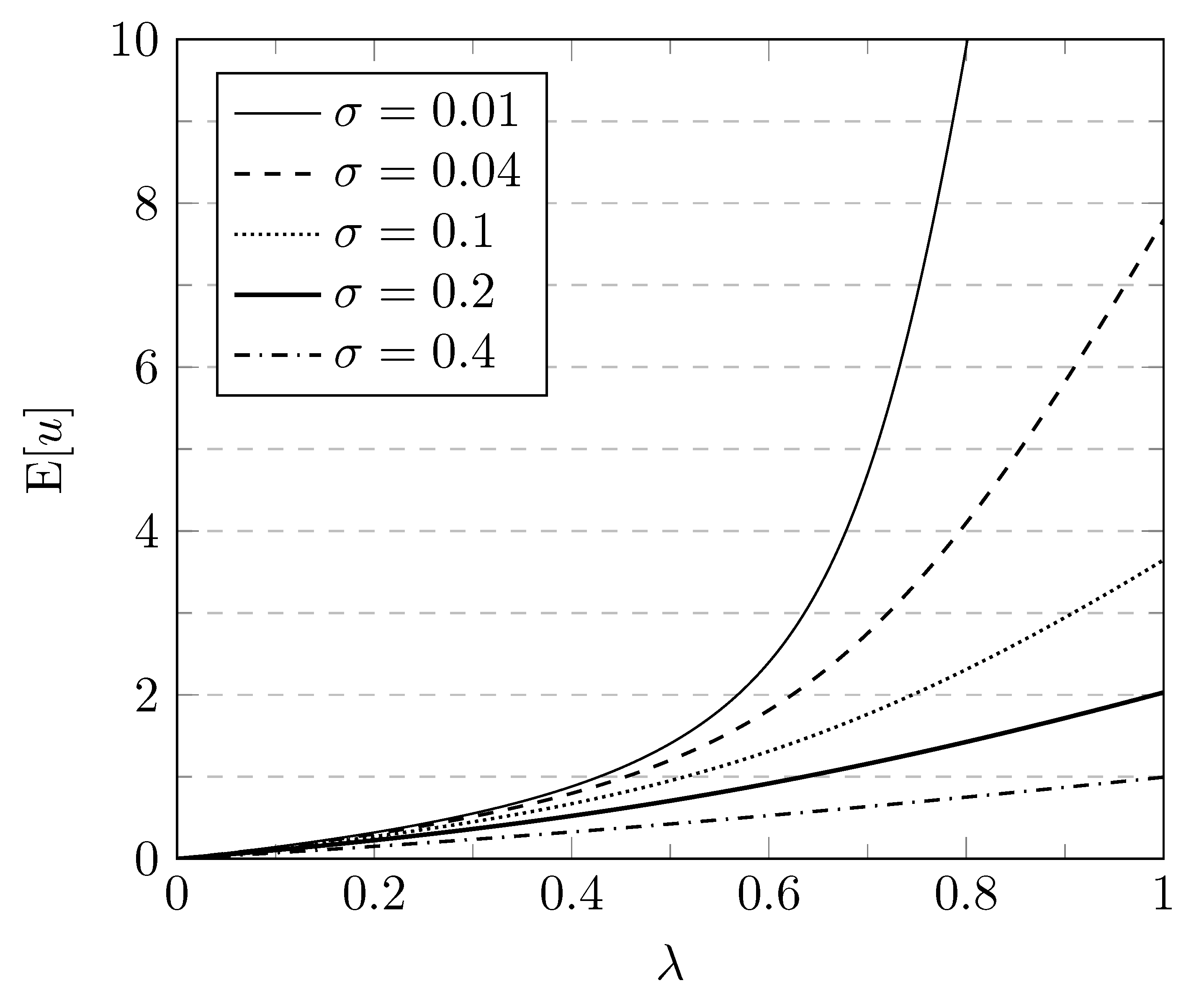
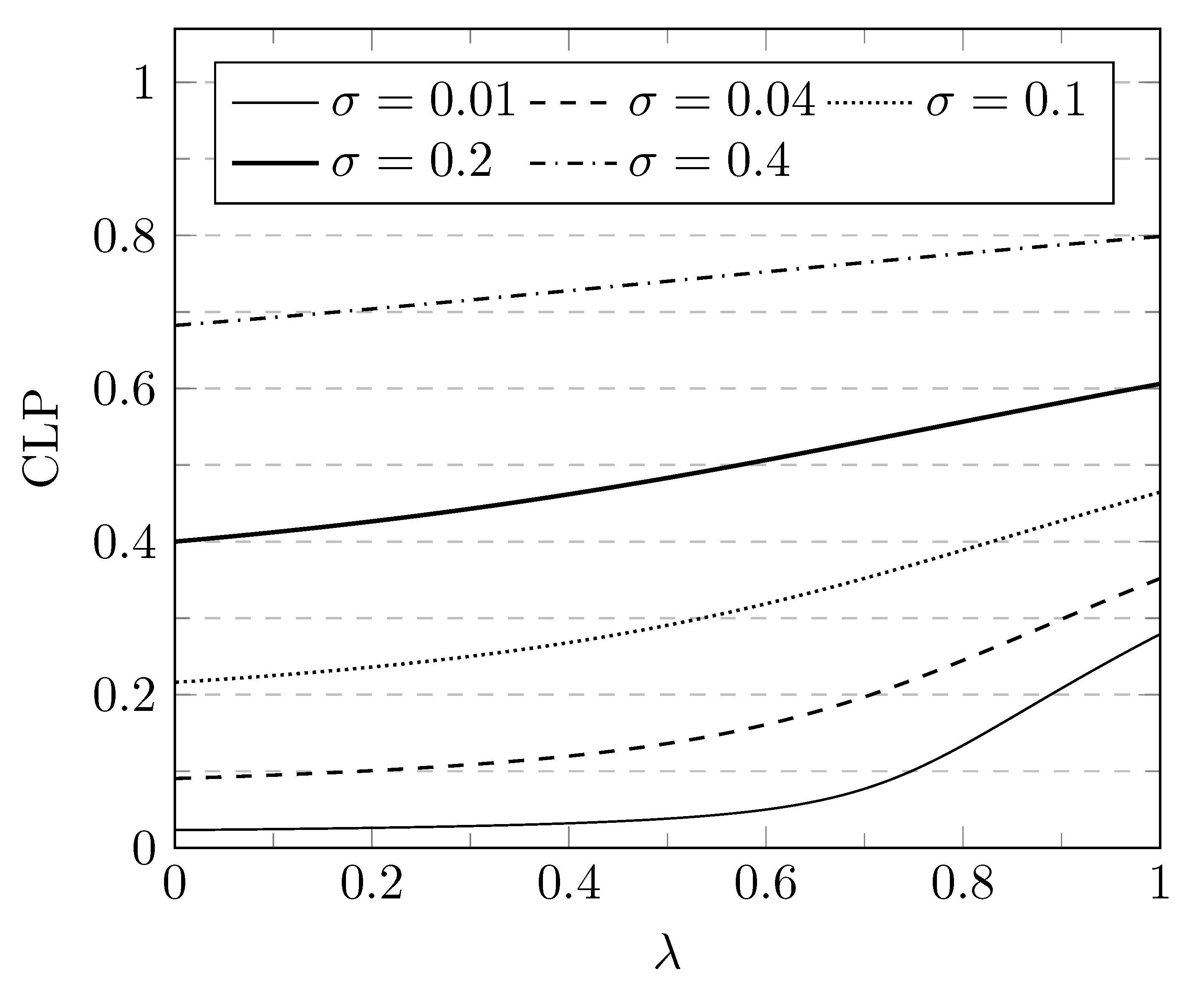
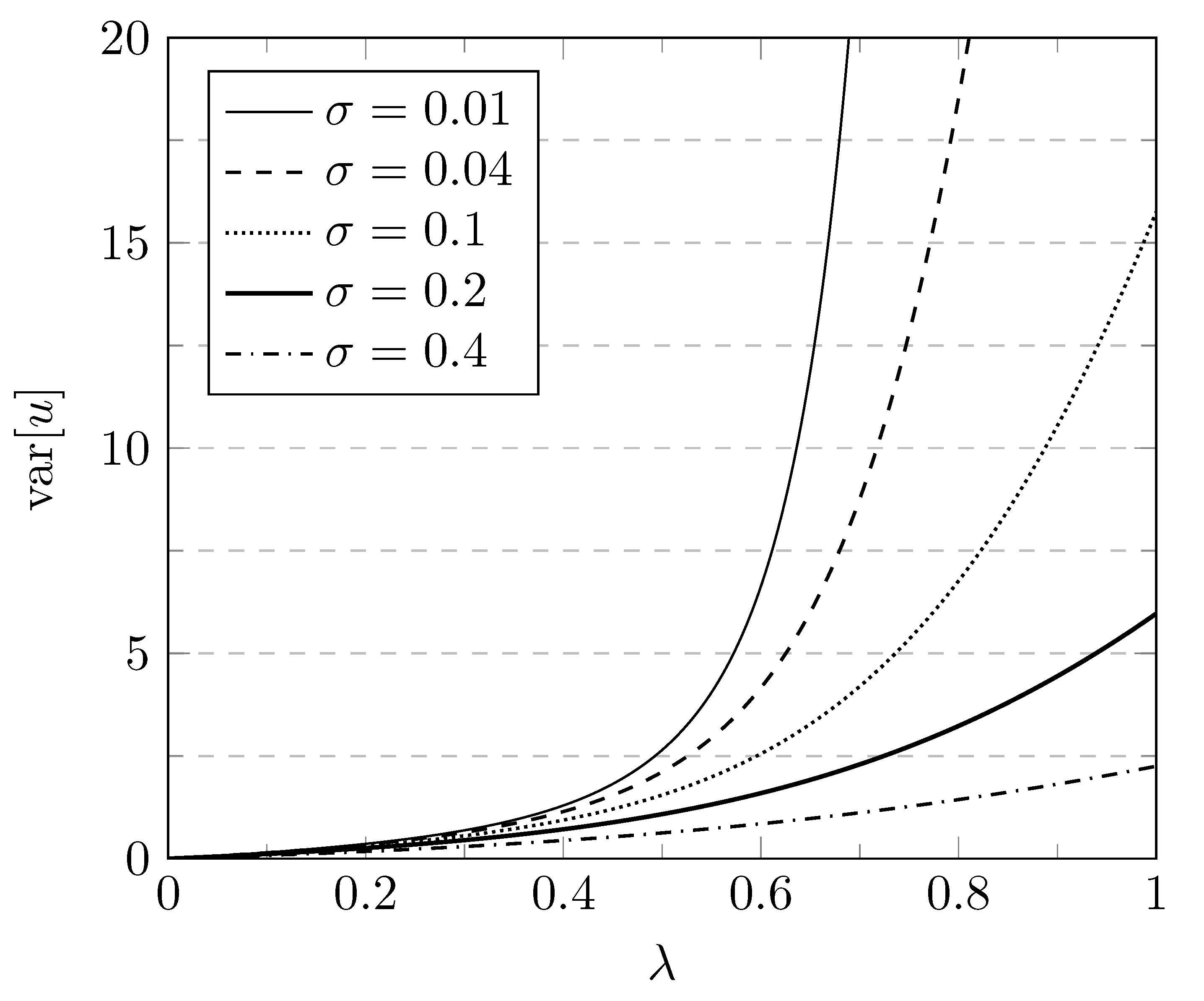
9. Numerical Examples

In order to illustrate the results obtained above, let us consider a number of numerical examples. In a first set of examples, in Figure 1, Figure 2, Figure 3 and Figure 4, we consider a Poisson distribution for the number of customer arrivals during a slot, i.e.,

$$A\left(z\right)=e^{\lambda (z-1)},$$

and a (shifted) geometric distribution for the service times, i.e.,

$$S\left(z\right)=\frac{\mu z}{1-(1-\mu )z},$$

with $\mu =0.75$ ($S^{\prime }\left(1\right)=\frac{1}{\mu }=1.33$). In Figure 1, the mean system content $\mathrm{E}\left[u\right]$ is plotted versus the arrival rate $\lambda$, for different values of the disaster probability $\sigma$. Similarly, Figure 2 shows the variance of the system content $\mathrm{var}\left[u\right]$, the mean sojourn time $\mathrm{E}\left[t\right]$ is plotted in Figure 3 and the customer loss probability is shown in Figure 4, all versus $\lambda$ for different values of $\sigma$. We observe that for an increasing disaster probability, $\mathrm{E}\left[u\right]$, $\mathrm{var}\left[u\right]$ and $\mathrm{E}\left[t\right]$ are decreasing, while $\mathrm{CLP}$ is increasing. This is clearly as intuitively expected. Indeed, the more often the system gets emptied due to a disaster occurrence (higher $\sigma$), the more customers are expected to get lost and the lower and less variable the system content and sojourn time thus become.

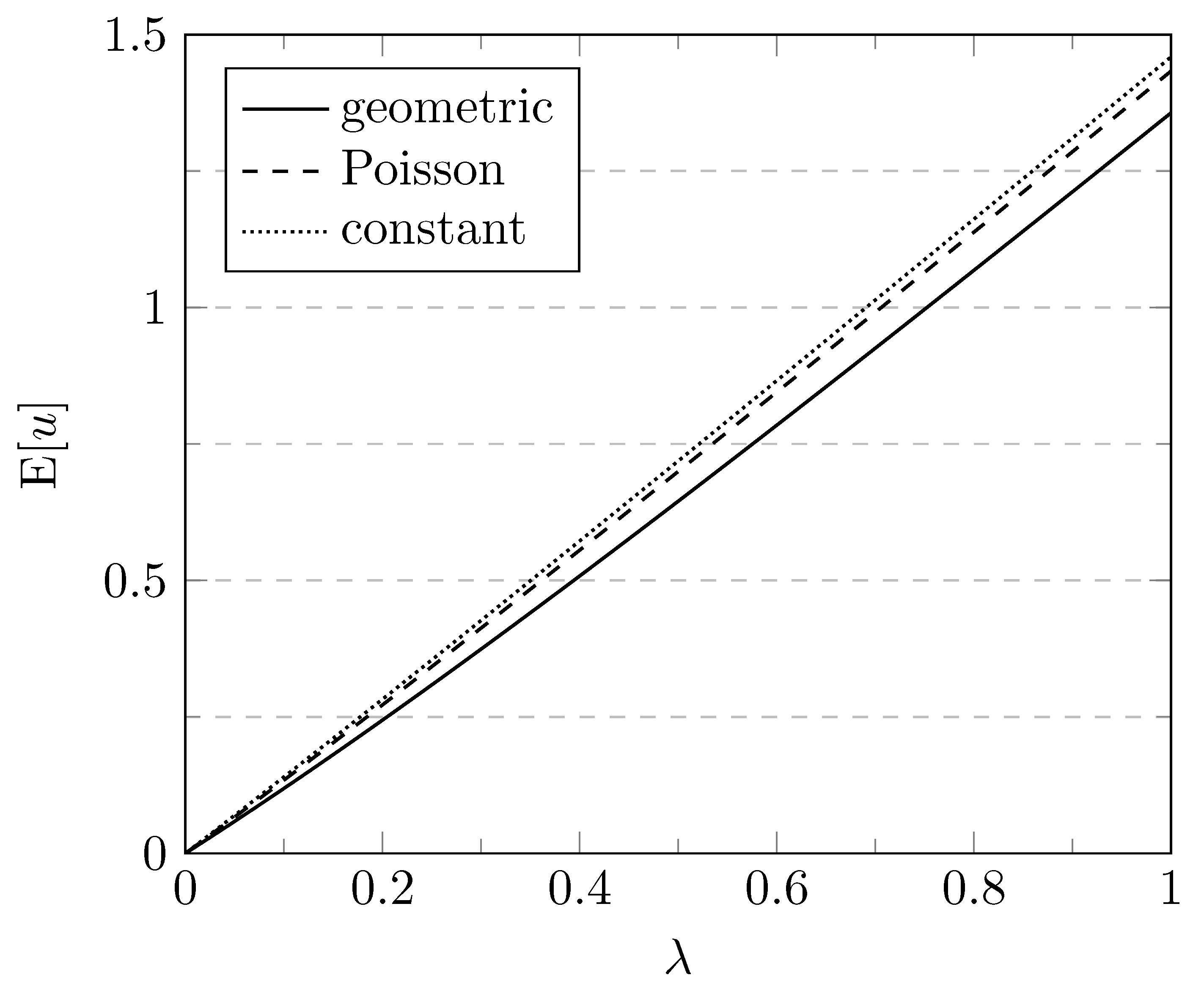
Next, in Figure 5, a number of different distributions are considered for the customer service times, all with the same mean service time $S^{\prime }\left(1\right)=\frac{1}{\mu }=5$: a (shifted) geometric distribution, a (shifted) Poisson distribution with

$$S\left(z\right)=z{e}^{(\frac{1}{\mu }-1)(z-1)}$$

and constant service times with

$$S\left(z\right)=z^{\frac{1}{\mu }}.$$

Figure 5 shows the mean system content versus $\lambda$, for Poisson arrivals and a disaster probability $\sigma =0.4$. For $S^{\prime }\left(1\right)=5$, the variance of the service times increases from 0 in the case of constant service times, to $\frac{1}{\mu }-1=4$ in the case of Poisson service times, and finally to $\frac{1-\mu }{{\mu }^2}=20$ in the case of geometric service times. We observe that $\mathrm{E}\left[u\right]$ decreases as the variance of the service times increases. Note that this is different from what is seen in classical queueing systems without disasters, where the mean system content typically increases with higher irregularity in the service times. The behavior of Figure 5 then follows from the fact that in the case of disaster occurrence, typically more customers are removed from the system when the service times are more variable, resulting in a lower system content on average.

In Figure 6, Figure 7 and Figure 8, we consider Poisson arrivals and a (shifted) Poisson distribution for the service times. In Figure 6, the mean system content is shown versus the mean service time $S^{\prime }\left(1\right)$ for $\lambda =0.4$ and various values of $\sigma$. Similarly, Figure 7 shows the variance $\mathrm{var}\left[u\right]$ of the system content, and Figure 8 shows the customer loss probability. From these figures, it can be seen that for a given value of $\lambda$, $\mathrm{E}\left[u\right]$, $\mathrm{var}\left[u\right]$ and $\mathrm{CLP}$ all increase with increasing values of $S^{\prime }\left(1\right)$, which could be expected due to the increasing system load $\lambda S^{\prime }\left(1\right)$. For increasing values of $\sigma$, we observe again that $\mathrm{E}\left[u\right]$ and $\mathrm{var}\left[u\right]$ are decreasing, while the loss probability increases, as is intuitively clear.

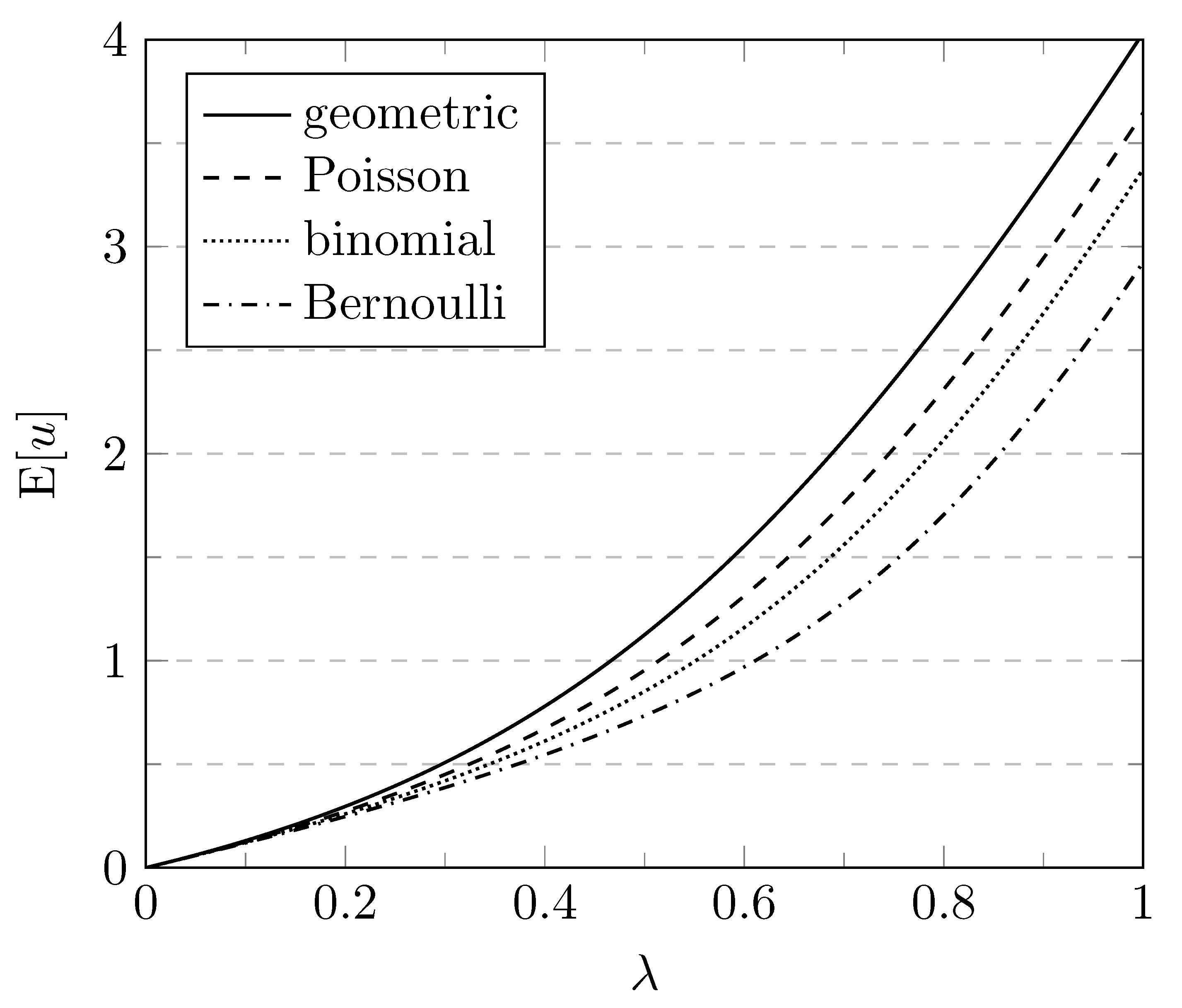
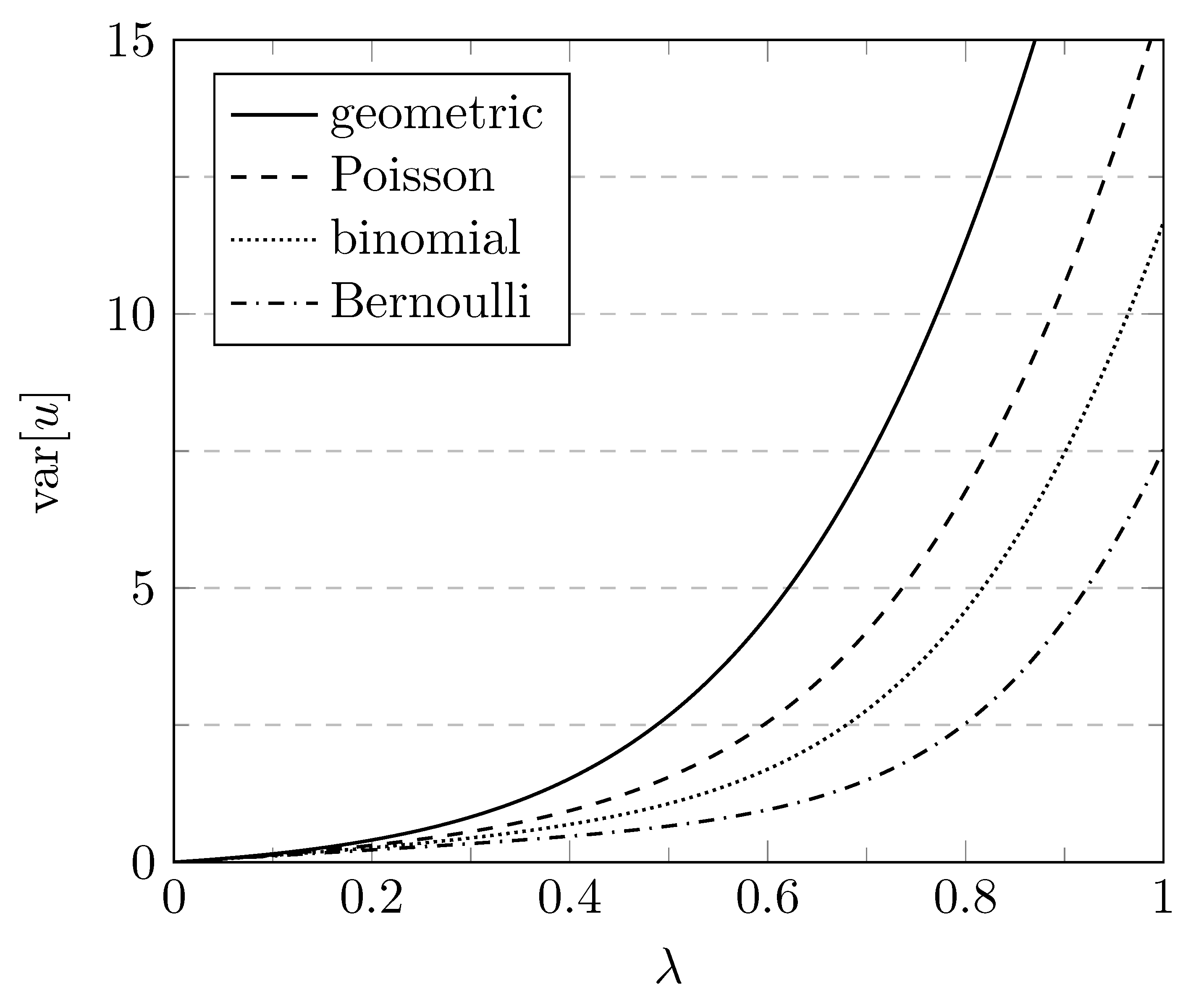
In Figure 9, Figure 10 and Figure 11, (shifted) geometric service times are considered with $\mu =0.75$. A number of different arrival distributions are considered, all with the same mean arrival rate $\lambda$: Poisson arrivals, Bernoulli arrivals, i.e.,

$$A\left(z\right)=1-\lambda +\lambda z,$$

geometric arrivals, i.e.,

$$A\left(z\right)=\frac{1}{1+\lambda -\lambda z},$$

and binomial arrivals, i.e.,

$$A\left(z\right)={\left(1-\frac{\lambda }{N}+\frac{\lambda }{N}z\right)}^N,$$

where $N=2$. Figure 9 and Figure 10 show the mean system content $\mathrm{E}\left[u\right]$ and the variance of the system content $\mathrm{var}\left[u\right]$ versus $\lambda$, for a fixed disaster probability $\sigma =0.1$. We observe that both $\mathrm{E}\left[u\right]$ and $\mathrm{var}\left[u\right]$ decrease in the order of geometric, Poisson, binomial and Bernoulli arrivals. This means that for given values of $\lambda$ and $\mu$, $\mathrm{E}\left[u\right]$ and $\mathrm{var}\left[u\right]$ decrease as the variance of the number of arrivals per slot decreases.

In Figure 11, the variance of the system content is plotted versus $\sigma$ for the same four arrival distributions with a fixed value of $\lambda =0.9$. For all arrival distributions, the variance $\mathrm{var}\left[u\right]$ decreases while the value of $\sigma$ is increasing, in accordance with the observations of Figure 2.

In Figure 12, the tail distribution of the system content is plotted on a logarithmic scale for (shifted) Poisson service times with $\mu =0.75$, Poisson arrivals with arrival rate $\lambda =1$ and different values of the disaster probability $\sigma$. For the same setting, Figure 13 shows the tail distribution of the sojourn time. We observe that, similar to the moments of the system content and the sojourn time, also the corresponding tail probabilities are decreasing functions of the disaster probability.

Finally,

Table 1. Tail probabilities, mean and variance of the system content u and the sojourn time t for Poisson arrivals with $\lambda =0.4$, Poisson service times with $\mu =0.2$ and different values of $\sigma$.

	$\mathit{\sigma }=0.05$		$\mathit{\sigma }=0.2$
$\mathit{n}$	$\mathrm{Prob}\left[\mathit{u}=\mathit{n}\right]$	$\mathrm{Prob}\left[\mathit{t}=\mathit{n}\right]$	$\mathrm{Prob}\left[\mathit{u}=\mathit{n}\right]$	$\mathrm{Prob}\left[\mathit{t}=\mathit{n}\right]$
10	$2.5647668\times {10}^{-2}$	$3.9904988\times {10}^{-2}$	$1.2037267\times {10}^{-3}$	$1.4136466\times {10}^{-2}$
20	$3.2333712\times {10}^{-3}$	$1.5896751\times {10}^{-2}$	$2.5425991\times {10}^{-6}$	$4.6894762\times {10}^{-4}$
30	$4.0762729\times {10}^{-4}$	$6.3327096\times {10}^{-3}$	$5.3706629\times {10}^{-9}$	$1.5556354\times {10}^{-5}$
40	$5.1389091\times {10}^{-5}$	$2.5227300\times {10}^{-3}$	$1.1344305\times {10}^{-11}$	$5.1604946\times {10}^{-7}$
50	$6.4785619\times {10}^{-6}$	$1.0049674\times {10}^{-3}$	$2.3962267\times {10}^{-14}$	$1.7118859\times {10}^{-8}$
60	$8.1674464\times {10}^{-7}$	$4.0034385\times {10}^{-4}$	$5.0614846\times {10}^{-17}$	$5.6788228\times {10}^{-10}$
70	$1.0296603\times {10}^{-7}$	$1.5948299\times {10}^{-4}$	$1.0691236\times {10}^{-19}$	$1.8838304\times {10}^{-11}$
80	$1.2980806\times {10}^{-8}$	$6.3532442\times {10}^{-5}$	$2.2582808\times {10}^{-22}$	$6.2492127\times {10}^{-13}$
90	$1.6364749\times {10}^{-9}$	$2.5309103\times {10}^{-5}$	$4.7701050\times {10}^{-25}$	$2.0730453\times {10}^{-14}$
100	$2.0630845\times {10}^{-10}$	$1.0082261\times {10}^{-5}$	$1.0075763\times {10}^{-27}$	$6.8768935\times {10}^{-16}$
	$\mathrm{E}\left[u\right]=4.663592380$		$\mathrm{E}\left[u\right]=1.292139933$
	$\mathrm{var}\left[u\right]=23.95418492$		$\mathrm{var}\left[u\right]=2.933050427$
	$\mathrm{E}\left[t\right]=11.65898095$		$\mathrm{E}\left[t\right]=3.230349832$
	$\mathrm{var}\left[t\right]=120.6749369$		$\mathrm{var}\left[t\right]=10.28852063$

presents some numerical results on the tail probabilities, the mean value and the variance of both the system content u and the sojourn time t for two different values of the disaster probability $\sigma$. We consider Poisson arrivals with $\lambda =0.4$ and Poisson service times with $\mu =0.2$ ($S^{\prime }\left(1\right)=\frac{1}{\mu }=5$).

10. Conclusions

In this paper, we studied the impact of disasters on the behavior of a discrete-time single-server queueing system under general probability distributions for both the number of customer arrivals during a slot and the length of the service time of a customer. Using a supplementary variable technique, we derived expressions for the pgfs, moments and tail probabilities of the system content and the sojourn time, and an expression for the customer loss probability due to disasters. Through numerical examples, the impact of disasters on the system characteristics was assessed. In contrast to classical queueing systems without disasters, we observed that for systems with disasters under a given system load, the mean system content decreases with increasing irregularity in the service times.

References

1. Gelenbe, E. Product-form queueing networks with negative and positive customers. J. Appl. Probab. 1991, 28, 656–663. [Google Scholar] [CrossRef]
2. Towsley, D.; Tripathi, S.K. A single server priority queue with server failures and queue flushing. Oper. Res. Lett. 1991, 10, 353–362. [Google Scholar] [CrossRef]
3. Atencia, I.; Moreno, P. The discrete-time Geo/Geo/1 queue with negative customers and disasters. Comput. Oper. Res. 2004, 31, 1537–1548. [Google Scholar] [CrossRef]
4. Jolai, F.; Asadzadeh, S.M.; Taghizadeh, M.R. Performance estimation of an email contact center by a finite source discrete time Geo/Geo/1 queue with disasters. Comput. Ind. Eng. 2008, 55, 543–556. [Google Scholar] [CrossRef]
5. Sudhesh, R.; Priya, R.; Lenin, R.B. Transient analysis of a single-server discrete-time queue with system disaster. RAIRO—Oper. Res. 2017, 51, 123–134. [Google Scholar] [CrossRef]
6. Yi, X.W.; Kim, J.D.; Choi, D.W.; Chae, K.C. The Geo/G/1 queue with disasters and multiple working vacations. Stoch. Model. 2007, 23, 537–549. [Google Scholar] [CrossRef]
7. Park, H.M.; Yang, W.S.; Chae, K.C. The Geo/G/1 queue with negative customers and disasters. Stoch. Model. 2009, 25, 673–688. [Google Scholar] [CrossRef]
8. Lee, D.H. Comments on ’Geo/G/1 queue with negative customers and disasters’. Stoch. Model. 2012, 28, 663–665. [Google Scholar] [CrossRef]
9. Lee, D.H.; Yang, W.S. The N-policy of a discrete time Geo/G/1 queue with disasters and its application to wireless sensor networks. Appl. Math. Model. 2013, 37, 9722–9731. [Google Scholar] [CrossRef]
10. Lee, D.H.; Yang, W.S.; Park, H.M. Geo/G/1 queues with disasters and general repair times. Appl. Math. Model. 2011, 35, 1561–1570. [Google Scholar] [CrossRef] [Green Version]
11. Yera, Y.G.; Fernández, C.A.; Valdés, J.E. A variant of the Geo/G/1 queues with disasters and general repair times. Commun. Stat.—Theory Methods 2019, 48, 6119–6133. [Google Scholar] [CrossRef]
12. Gao, S.; Wang, J.; Do, T.V. Analysis of a discrete-time repairable queue with disasters and working breakdowns. RAIRO—Oper. Res. 2019, 53, 1197–1216. [Google Scholar] [CrossRef] [Green Version]
13. Park, H.M.; Yang, W.S.; Chae, K.C. Analysis of the GI/Geo/1 queue with disasters. Stoch. Anal. Appl. 2010, 28, 44–53. [Google Scholar] [CrossRef]
14. Wang, J.; Huang, Y.; Do, T.V. A single-server discrete-time queue with correlated positive and negative customer arrivals. Appl. Math. Model. 2013, 37, 6212–6224. [Google Scholar] [CrossRef]
15. Sudhesh, R.; Vaithujanathan, A. Analysis of state-dependent discrete-time queue with system disaster. RAIRO—Oper. Res. 2019, 53, 1915–1927. [Google Scholar] [CrossRef]
16. Atencia, I.; Moreno, P. A single-server G-queue in discrete-time with geometrical arrival and service process. Perform. Eval. 2005, 59, 85–97. [Google Scholar] [CrossRef] [Green Version]
17. Zhou, W.-H. Performance analysis of discrete-time queue GI/G/1 with negative arrivals. Appl. Math. Comput. 2005, 170, 1349–1355. [Google Scholar] [CrossRef]
18. Wang, J.; Zhang, P. A discrete-time retrial queue with negative customers and unreliable server. Comput. Ind. Eng. 2009, 56, 1216–1222. [Google Scholar] [CrossRef]
19. Wang, J.; Zhang, P. A single-server discrete-time retrial G-queue with server breakdowns and repairs. Acta Math. Appl. Sin. (Engl. Ser.) 2009, 25, 675–684. [Google Scholar] [CrossRef]
20. Chae, K.C.; Park, H.M.; Yang, W.S. A GI/Geo/1 queue with negative and positive customers. Appl. Math. Model. 2010, 34, 1662–1671. [Google Scholar] [CrossRef]
21. Wang, J.; Huang, Y.; Dai, Z. A discrete-time on-off source queueing system with negative customers. Comput. Ind. Eng. 2011, 61, 1226–1232. [Google Scholar] [CrossRef]
22. Gao, S.; Wang, J.; Zhang, D. Discrete-time GIX/Geo/1/N queue with negative customers and multiple working vacations. J. Korean Stat. Soc. 2013, 42, 515–528. [Google Scholar] [CrossRef]
23. Ma, Z.; Guo, Y.; Wang, P.; Hou, Y. The Geo/Geo/1+1 queueing system with negative customers. Math. Probl. Eng. 2013, 2013. [Google Scholar] [CrossRef] [Green Version]
24. Do, T.V. An initiative for a classified bibliography on G-networks. Perform. Eval. 2011, 68, 385–394. [Google Scholar] [CrossRef]
25. Do, T.V. Bibliography on G-networks, negative customers and applications. Math. Comput. Model. 2011, 53, 205–212. [Google Scholar] [CrossRef]
26. Peng, Y.; Yang, X.Q. On a BMAP/G/1 G-queue with setup times and multiple vacations. Acta Math. Appl. Sin. (Engl. Ser.) 2011, 27, 625–638. [Google Scholar] [CrossRef]
27. Klimenok, V.; Dudin, A. A BMAP/PH/N queue with negative customers and partial protection of service. Commun. Stat.—Simul. Comput. 2012, 41, 1062–1082. [Google Scholar] [CrossRef]
28. Do, T.V.; Papp, D.; Chakka, R.; Sztrik, J.; Wang, J. M/M/1 retrial queue with working vacations and negative customer arrivals. Int. J. Adv. Intell. Paradig. 2014, 6, 52–65. [Google Scholar] [CrossRef] [Green Version]
29. Zhang, M.; Liu, Q. An M/G/1 G-queue with server breakdown, working vacations and vacation interruption. Opsearch 2015, 52, 256–270. [Google Scholar] [CrossRef]
30. Jiang, T.; Liu, L. Analysis of a GI/M/1 queue in a multi-phase service environment with disasters. RAIRO—Oper. Res. 2017, 51, 79–100. [Google Scholar] [CrossRef]
31. Jiang, T.; Liu, L. The GI/M/1 queue in a multi-phase service environment with disasters and working breakdowns. Int. J. Comput. Math. 2017, 94, 707–726. [Google Scholar] [CrossRef]
32. Chin, C.H.; Koh, S.K.; Tan, Y.F.; Pooi, A.H.; Goh, Y.K. Stationary queue length distribution of a continuous-time queueing system with negative arrival. J. Phys. Conf. Ser. 2018, 1132, 012057. [Google Scholar] [CrossRef]
33. Peng, Y. The MAP/G/1 G-queue with unreliable server and multiple vacations. Inform.-J. Comput. Inform. 2019, 43, 545–550. [Google Scholar] [CrossRef] [Green Version]
34. Kumar, N.; Barbhuiya, F.P.; Gupta, U.C. Unified killing mechanism in a single server queue with renewal input. Opsearch 2020, 57, 246–259. [Google Scholar] [CrossRef]
35. Gupta, U.C.; Kumar, N.; Barbhuiya, F.P. A queueing system with batch renewal input and negative arrivals. In Applied Probability and Stochastic Processes; Springer: Singapore, 2020; pp. 143–157. [Google Scholar]
36. Kumar, N.; Gupta, U.C. Analysis of BMAP/MSP/1 queue with MAP generated negative customers and disasters. Commun. Stat.—Theory Methods 2021. [Google Scholar] [CrossRef]
37. Bruneel, H.; Maertens, T. A discrete-time queue with customers with geometric deadlines. Perform. Eval. 2015, 85–86, 52–70. [Google Scholar] [CrossRef] [Green Version]
38. Bruneel, H.; Steyaert, B.; Desmet, E.; Petit, G.H. Analytic derivation of tail probabilities for queue lengths and waiting times in ATM multiserver queues. Eur. J. Oper. Res. 1994, 76, 563–572. [Google Scholar] [CrossRef]
39. Bruneel, H.; Kim, B.G. Discrete-Time Models for Communication Systems Including ATM; Kluwer Academic Publishers: Boston, MA, USA, 1993. [Google Scholar]
40. González, M.O. Classical Complex Analysis; Marcel Dekker: New York, NY, USA, 1992. [Google Scholar]
Figure 1. Mean system content E u versus λ , for Poisson arrivals, geometric service times with μ = 0.75 and different values of σ .
Mathematics 09 03283 g001
Figure 2. Variance of the system content var u versus λ , for Poisson arrivals, geometric service times with μ = 0.75 and different values of σ .
Mathematics 09 03283 g002
Figure 3. Mean sojourn time E t versus λ , for Poisson arrivals, geometric service times with μ = 0.75 and different values of σ .
Mathematics 09 03283 g003
Figure 4. Customer loss probability CLP versus λ for Poisson arrivals, geometric service times with μ = 0.75 and different values of σ .
Mathematics 09 03283 g004
Figure 5. Mean system content E u versus λ , for Poisson arrivals, σ = 0.4 and various distributions for the service times with S ( 1 ) = 5 .
Mathematics 09 03283 g005
Figure 6. Mean system content E u versus S ( 1 ) for Poisson service times, Poisson arrivals with λ = 0.4 and different values of σ .
Mathematics 09 03283 g006
Figure 7. Variance of the system content var u versus S ( 1 ) for Poisson service times, Poisson arrivals with λ = 0.4 and different values of σ .
Mathematics 09 03283 g007
Figure 8. Customer loss probability CLP versus S ( 1 ) for Poisson service times, Poisson arrivals with λ = 0.4 and different values of σ .
Mathematics 09 03283 g008
Figure 9. Mean system content E u versus λ for geometric service times with μ = 0.75 , σ = 0.1 and various distributions for the number of arrivals per slot.
Mathematics 09 03283 g009
Figure 10. Variance of the system content var u versus λ for geometric service times with μ = 0.75 , σ = 0.1 and various distributions for the number of arrivals per slot.
Mathematics 09 03283 g010
Figure 11. Variance of the system content var u versus σ , for geometric service times with μ = 0.75 , λ = 0.9 and various distributions for the number of arrivals per slot.
Mathematics 09 03283 g011
Figure 12. Tail distribution of the system content Prob u = n versus n for Poisson service times with μ = 0.75 , Poisson arrivals with λ = 1 and different values of σ .
Mathematics 09 03283 g012
Figure 13. Tail distribution of the sojourn time Prob t = n versus n for Poisson service times with μ = 0.75 , Poisson arrivals with λ = 1 and different values of σ .
Mathematics 09 03283 g013