Article

Spatio-Temporal Modeling of Immune Response to SARS-CoV-2 Infection

Mathematics Department, Al-Qunfudhah University College, Umm Al-Qura University, Al-Qunfudhah 28821, Saudi Arabia
Mathematics 2021, 9(24), 3274; https://doi.org/10.3390/math9243274
Submission received: 23 November 2021 / Revised: 9 December 2021 / Accepted: 14 December 2021 / Published: 16 December 2021
(This article belongs to the Section Mathematical Biology)

Abstract

:
COVID-19 is a disease occurring as a result of infection by a novel coronavirus called SARS-CoV-2. Since the WHO announced COVID-19 as a global pandemic, mathematical works have taken place to simulate infection scenarios at different scales even though the majority of these models only consider the temporal dynamics of SARS-COV-2. In this paper, we present a new spatio-temporal within-host mathematical model of COVID-19, accounting for the coupled dynamics of healthy cells, infected cells, SARS-CoV-2 molecules, chemokine concentration, effector T cells, regulatory T cells, B-lymphocytes cells and antibodies. We develop a computational framework involving discretisation schemes for diffusion and chemotaxis terms using central differences and midpoint approximations within two dimensional space combined with a predict–evaluate–correct mode for time marching. Then, we numerically investigate the model performance using a list of values simulating the baseline scenario for viral infection at a cellular scale. Moreover, we explore the model sensitivity via applying certain conditions to observe the model validity in a comparison with clinical outcomes collected from recent studies. In this computational investigation, we have a numerical range of 104 to 108 for the viral load peak, which is equivalent to what has been obtained from throat swab samples for many patients.

1. Introduction

In December 2019, the coronavirus disease 2019 (COVID-19) was first identified in Wuhan and rapidly invaded the whole of China and the world [1]. This disease was officially named COVID-19 by the World Health Organization (WHO) on 11 January 2020; then it was announced as a global health emergency on 11 March 2020 [2,3]. Since then, many studies have been done to investigate this global pandemic. As a part of these efforts, we here aim to develop a mathematical model to describe and simulate the interactions between SARS-CoV-2 molecules and the immune system within a two dimensional cellular space. In the following, we present a brief overview of SARS-CoV-2 in terms of its spreading properties, viral replication and mechanism of infection.
Severe acute respiratory syndrome coronavirus 2 (SARS-CoV-2) is a novel virus that has a genetic similarity to SARS-CoV, which is responsible for SARS disease, while the new virus (SARS-CoV-2) causes coronavirus disease 19 (COVID-19) [4]. Both SARS-CoV and SARS-CoV-2 have a common link in terms of mechanism of infection where both of them use the spike proteins (S-protein) to bind Angiotensin-converting enzyme 2 (ACE2), which in turn helps them to reach and attack the cells [4]. Despite this similarity, it has been found that SARS-CoV-2 binds to ACE2 slower than the old virus (SARS-CoV) where this slow binding causes a longer incubation period. Hence, this time delay of onset symptoms of COVID-19 leads to a faster spread of the pandemic around the world [3].
Although there is a lack of enough experimental studies about immune responses for people who have symptomatic/asymptomatic COVID-19 infections, there are some studies which investigate the interactions between the virus and many components of the immune system including the innate and the adaptive immune responses [5,6,7]. Once coronavirus-2 gains access inside the host cell using its spike protein (S) and the target cell receptor (ACE2) (in the same manner as SARS-CoV), it begins uncovering its genetic materials and producing some essential proteins such as envelope (E), nucleocapsid (N) and also spike (S) for motivating the interactions with target cells as well as assembling and releasing a new virus generation [8,9]. The ability of viral replication drives to having a local inflammatory response which motivates the immune system to recognize the virus and start the primary line of defense, that is, the activation of neutrophils, natural killer cells, naive T and B cells and the secretion of chemokine [10,11]. As long as the infection persists for a certain period of time, T cells pass through many stages including their proliferation, activation, migration, and differentiation, ultimately they come in the form of the effector T cells involving both helper (CD4+) and cytotoxic T cells (CD8+), and the regulatory T cells (Treg) [10]. Besides the cellular immunity, B cells play a key role in humoral immunity, especially after their transformation into plasma B cells (via the assistance of the armed/follicular helper T cells [10,12,13]). These types of cells have the ability to produce antibodies specific to SARS-CoV-2, such as IgA, IgG, and IgM, in order to neutralize the virus at the infection site [4,8,14]. Antibodies specific to SARS-CoV-2 are mostly a very essential tool for neutralizing the virus via decreasing its binding ability to ACE2, but we should take into account its potential threat of enhancing the immunopathogenesis [15]. However, there is biological evidence that shows that the antibody levels are going to be decreased over time through infection with SARS-CoV-2, while particular components of the immune system, such as the memory T/B cells, will maintain at a high level for almost 6 to 8 months [6].
One major obstacle that creates difficulties for dealing with SARS-CoV-2 infection is the quick activation and migration of T cells to the site of viral replication, which in turn leads to releasing a huge amount of inflammatory cytokines such as IL-1, IL-6, and IFN- γ . This storm of cytokines causes the cytokine release syndrome resulting in serious damage to vital organs such as lungs as well as causing viral sepsis [11,16]. On other hand, there is no clue so far suggesting that the evolution of B cells over time will participate in this pathogenesis. However, we cannot generalize this scenario because it has been found that some of infected patients with SARS-CoV-2 who were treated in the ICU or who died have low levels of T cells as well as B cells [7].
Over the past decades, mathematical modeling of immune responses to viral infections has developed in terms of either realizing the biological concepts or improving the mathematical techniques to obtain better outputs [17,18,19,20]. Since the outbreak of COVID-19, many mathematical research projects have been performed, but the majority of these mathematical models focus on the temporal dynamics only (ODE models) which either use the so-called SIR-models (compartmental models) to predict the population progress between compartments such as [21,22,23,24,25], or describe the within host dynamics to investigate immune responses to SARS-CoV-2 particles within the cellular scale as proposed in [22,26,27]. However, these within host models were being built on previous studies for similar infectious diseases such as influenza [18,28] and hepatitis B [29]. To our knowledge, we could not find any spatio-temporal model for describing the spatial distribution of the immune responses to SARS-CoV-2 within a two dimensional cellular space. Nevertheless, there are a few preprint mathematical studies using PDEs to describe the spread of the population compartments with respect to time and their physical locations at different regions which means these mathematical approaches are still a type of the compartmental class models. Therefore, in Section 2, we present a first attempt for deriving a new mathematical model, which is based on a coupled system of partial differential equations to obtain a reasonable description for the interaction between coronavirus-2 and its response to the components of immune system.
The rest of this paper is summarized as follows. Section 3 includes model calibration and developing a computational framework to compute the coupled reaction diffusion system within two spatial dimensions. Section 4 involves a comparison of our numerical results with a few cases collected from recent clinical studies. Lastly, in Section 5 we present a discussion on a few key points including hints at future works.

2. Modeling Framework

Building on some biological observations and mathematical models (temporal approaches) [7,8,10,11,12,13,16,22,28,30,31,32,33,34,35,36], we develop a new spatio-temporal mathematical model to explore the interactions between the most essential components of the immune system and SARS-CoV-2 particles within a cellular perspective. This dynamical interaction occurs on a spatial domain R 2 over a time interval [ 0 , T ] and it involves the healthy host cells h ( t , x ) , viral-infected cells i ( t , x ) , SARS-CoV-2 molecules v ( t , x ) , chemokines c ( t , x ) , the effector T cells f ( t , x ) , the regulatory T cells r ( t , x ) , B-lymphocytes cells β ( t , x ) and antibodies α ( t , x ) . In a similar manner to the modeling derivation method under a continuum approach and the conservation law as detailed in [37], we assume that L is a fixed (random) volume surrounded entirely by a smooth surface Z . Then, the appearance or disappearance of any component within L is expressed by the flux of that component through the boundary Z and the proliferation and/or degradation of that component. In other words, we suppose that C represents the concentration of a component at a fixed time t and a position x = ( x , y ) , J denotes the net flow of a component and P stands for the proliferation and/or the degradation of a component. Hence, we have the following conservation equation:
d dt L C ( x , t ) dx = Z J ( x , t ) d Z + L P d L ,
where Z = L . Now, using the divergence theorem, we can differentiate to get the following conservation equation for each component of a system, namely,
C t = · J + P .
The above method has been used to model many biological applications such as [34,38,39,40]. Thus, we can denote the resulting 8D-reaction-diffusion-chemotaxis operator K by the following expression:
K ( h , i , v , c , f , r , β , α ) T = 0 ,
where the differential operator ( K ) of order 2 will be explained in detail in the following context.
Host h ( t , x ) & Infected cells i ( t , x ) Following biological observations and spatio-temporal mathematical approach that have been taken from various experimental studies for similar infectious diseases such as [31,32], we suppose that both type of cells are exercising a random motility on the spatial domain at rates D h > 0 and D i > 0 , respectively. The density of the host cells is assumed to be produced logistically at a rate μ h , while the decay of its density comes from many reasons at a rate δ 11 . At the same time, the infected cells are produced when SARS-CoV-2 virus binds the host cells by the S protein at a rate μ i through the targeted receptor, namely, ACE2 [11]. Moreover, the density of infected cells is decreased over time due to two main factors, namely, effector T cells f ( t , x ) at a rate δ 21 [10,33] and natural deaths at a rate δ 22 . These assumptions can be formalised mathematically through the following expressions:
h t = D h 2 h + μ h h ( 1 h h 0 ) δ 11 h , i t = D i 2 i + μ i h v δ 21 i f δ 22 i .
SARS-CoV-2 v ( t , x ) As mentioned in [8], SARS-CoV-2 has the ability to motile inside the respiratory system, therefore, we assume that coronavirus-2 diffuses randomly through at a random motility rate D v . Furthermore, the interactions between immune cells and viruses increase the secretion level of chemokines, which in turn impacts virus movement [8]. Adopting this assumption, we suppose that SARS-CoV-2 migration is directed towards a higher concentration of a chemical gradient at a rate χ v . Moreover, coronaviruses are capable of viral replication actively within throat for at least 5 days (depending on the duration of the onset of symptoms) as detailed in the clinical studies [41,42], where this viral replication occurs due to the existence of the gene (ORF1) [36]. Hence, we take into account its replication within infected cells at a rate μ v . However, besides the natural decay of SARS-CoV-2 density at a rate δ 32 , the antibodies (produced by B cells) play a key role in restricting or preventing virus entry inside the host cells [10], hence SARS-CoV-2 particles are assumed to be decreased due to antibodies increasing level at a rate δ 31 . These words can be mathematically expressed via the following equation:
v t = D v 2 v χ v · ( v c ) + μ v i δ 31 α v δ 32 v .
Chemokine Concentration c ( t , x ) Chemokines are small proteins secreted by many cells where they have the ability to direct the surrounding cells chemotaxically towards the source of the chemokines [43]. Besides the homeostatic function of chemokines [43], chemokines have been found in many COVID-19 patients [8,10] for attracting immune cells towards the inflammatory sites [8]. Thus, it is assumed to be produced proportionally to the viral-infected cells and T cells at a rate μ c , with taking into consideration its natural decay at a rate δ 41 . Moreover, we suppose that chemokines can move randomly through the tissue at a random motility coefficient rate D c . Therefore, we have the following equation:
c t = D c 2 c + μ c i f δ 41 c .
The effector f ( t , x ) and the regulatory T cells r ( t , x ) In general, T cells are one of the most important components of immune system un which they play a key role in the initiation of the adaptive immune responses during the immunity cycle [10]. Regardless of the complexity of T cells functions and multi-stage processes including naive, helper, cytotoxic and memory T cells, it ultimately turns into the effector T cells ( f ( t , x ) ) [10]. Additionally, we also account for the dynamics of the regulatory T cells ( r ( t , x ) ) due to its significant role in immune homeostasis and in controlling the proliferation of effector T cells [30]. Biological evidence shows that the efficiency of T cells depends on its motility pattern, spatial distribution and motility major obstacles [33]. Therefore, we take into account the random movement on the spatial domain for both T cells (effector and regulatory) with motility rates D f and D r , respectively [7,34]. In addition to that, the directional migration of T cells is assumed to be in the form of chemotaxis towards gradients of the secreted chemokines (with the chemotaxic rates χ f , χ r ) [7,8,33,34]). Building on relevant studies [28,35], this specific study [22] proposes a model describing the proliferation form of T cells in the context of COVID-19. Thus, we assume that the proliferation of the effector T cells arises naturally at a rate μ f and its growth depends on the virus distribution with taking into consideration the maximum carrying capacity k f . Furthermore, the proliferation rate of the regulatory T cells keeps track of the production of the effector T cells at a rate μ r with a carrying capacity rate k r . However, both types of T cells are supposed to be decreased naturally at rates δ 52 and δ 61 , respectively. Besides this, the regulatory T cells regulate the immune system and also suppress the proliferation of effector T cells before damage occurs [30]. Consequently, this interaction between the two types of T cells leads to a decay in the overall density of the effector T cells at a rate δ 51 . Hence, the evolution of the effector and the regulatory T cells are represented by the following equations:
f t = D f 2 f χ f · ( f c ) + μ f v v + k f δ 51 r f δ 52 f , r t = D r 2 r χ r · ( r c ) + μ r f f + k r δ 61 r .
B-lymphocytes cells β ( t , x ) & Antibodies α ( t , x ) During the early stages of infection with the SARS-CoV-2 virus, T cells (armed/follicular helper T cells) and their released cytokines during activation play an important role in the activation process of B cells [12,13,16] including the early responses of B cells against the N protein [8]. Therefore, we suppose that the production level of T cells increases the activation level of B cells at a rate μ β ˜ . Moreover, the proliferation of B cells is caused via virus growth tracking at a rate μ β with a maximum carrying capacity k β . Meanwhile, its density decay is naturally occurring at a rate δ 71 . Furthermore, we account for the produced antibodies by B cells at a rate μ α [7,10]. However, the density of antibodies is assumed to be degraded due to inhibition induced via binding with SARS-CoV-2 as well as by natural reasons at a rate δ 81 [7,10]. Both B cells and antibodies are assumed to exercise a random motility on the spatial domain at diffusion coefficients D β and D α , respectively. We also take into account the chemotaxis directional movement of B cells towards inflammatory concentration [8,10] at a rate χ β . The above assumptions are formalised mathematically by the following equations:
β t = D β 2 β χ β · ( β c ) + μ β v v + k β + μ β ˜ f δ 71 β , α t = D α 2 α + μ α β δ 81 α .
Considering the above modeling hypotheses, the full model is written as follows:
h t = D h 2 h + μ h h ( 1 h h 0 ) δ 11 h , i t = D i 2 i + μ i h v δ 21 i f δ 22 i , v t = D v 2 v χ v · ( v c ) + μ v i δ 31 α v δ 32 v , c t = D c 2 c + μ c i f δ 41 c , f t = D f 2 f χ f · ( f c ) + μ f v v + k f δ 51 r f δ 52 f , r t = D r 2 r χ r · ( r c ) + μ r f f + k r δ 61 r , β t = D β 2 β χ β · ( β c ) + μ β v v + k β + μ β ˜ f δ 71 β , α t = D α 2 α + μ α β δ 81 α .
Each of the above coupled dynamics are followed by initial and boundary conditions which will be given in detail in Section 3.2.

3. Model Calibration and Computational Approach

In this section, we aim to prepare our dynamical system to be solved numerically and to provide a realistic simulation in the hope that it will coincide with a range of clinical findings. To this done, we first rewrite model (7) in a dimensionless form, then we select the initial seeds for system components involving shapes and quantities. Then, we calibrate the model and develop a numerical scheme to represent a scenario for immune responses to SARS-CoV-2 infection based on experimental data.

3.1. Non-Dimensionalization

To explore the performance of our proposed spatio-temporal model (7), we begin with non-dimensionalising the system in order to remove the physical dimensions of the variables to solve the system numerically. To that end, we rescale the space variable x : = ( x , y ) to be related to the length of the considered region, namely, L = 0.1 cm in parallel with rescaling time with a reasonable scaling parameter τ = L 2 D where D = 10 6 c m 2 s is the spatial chemical diffusion rate as referenced in [44]. Based on that, we have τ = 10 4 s which is equivalent to about 2.78 h. Now, we rewrite the dependent variables as follows: h ¯ ( t ¯ , x ¯ , y ¯ ) = h ( t , x , y ) h 0 , i ¯ ( t ¯ , x ¯ , y ¯ ) = i ( t , x , y ) i 0 , v ¯ ( t ¯ , x ¯ , y ¯ ) = v ( t , x , y ) v 0 , c ¯ ( t ¯ , x ¯ , y ¯ ) = c ( t , x , y ) c 0 , f ¯ ( t ¯ , x ¯ , y ¯ ) = f ( t , x , y ) f 0 , r ¯ ( t ¯ , x ¯ , y ¯ ) = r ( t , x , y ) r 0 , β ¯ ( t ¯ , x ¯ , y ¯ ) = β ( t , x , y ) β 0 and α ¯ ( t ¯ , x ¯ , y ¯ ) = α ( t , x , y ) α 0 where t ¯ = t τ , x ¯ = x L , y ¯ = y L , while h 0 , i 0 , v 0 , c 0 , f 0 , r 0 , β 0 and α 0 are proper fixed parameters. Furthermore, for the remaining variables, we select the following key parameters: D ¯ h = D h τ L 2 = D h D , μ ¯ h = μ h τ , δ ¯ 11 = δ 11 τ , D ¯ i = D i τ L 2 = D i D , μ i ¯ = μ i τ h 0 v 0 i 0 , δ ¯ 21 = δ 21 τ f 0 , δ ¯ 22 = δ 22 τ , D ¯ v = D v τ L 2 = D v D , χ ¯ v = χ v c 0 τ L 2 , μ ¯ v = μ v τ i 0 v 0 , δ ¯ 31 = δ 31 τ α 0 , δ ¯ 32 = δ 32 τ , D ¯ c = D c τ L 2 = D c D , μ ¯ c = μ c τ i 0 f 0 c 0 , δ ¯ 41 = δ 41 τ , D ¯ f = D f τ L 2 = D f D , χ ¯ f = χ f c 0 τ L 2 , μ ¯ f = μ f τ f 0 , k ¯ f = k f v 0 , δ ¯ 51 = δ 51 τ r 0 , δ ¯ 52 = δ 52 τ , D ¯ r = D r τ L 2 = D r D , χ ¯ r = χ r c 0 τ L 2 , μ ¯ r = μ r τ r 0 , k ¯ r = k r f 0 , δ ¯ 61 = δ 61 τ , D ¯ β = D β τ L 2 = D β D , χ ¯ β = χ β c 0 τ L 2 , μ ¯ β = μ β τ β 0 , k ¯ β = k β v 0 , μ ¯ β ˜ = μ β ˜ τ f 0 β 0 , δ ¯ 71 = δ 71 τ , D ¯ α = D α τ L 2 = D α D , μ ¯ α = μ α τ β 0 α 0 , δ ¯ 81 = δ 81 τ . Subsequently, we substitute the above rescaled variables into the coupled reaction diffusion system (7) to obtain the following dimensionless version with removing the over-lines for easier readability:
h t = D h 2 h + μ h h ( 1 h ) δ 11 h , i t = D i 2 i + μ i h v δ 21 i f δ 22 i , v t = D v 2 v χ v · ( v c ) + μ v i δ 31 α v δ 32 v , c t = D c 2 c + μ c i f δ 41 c , f t = D f 2 f χ f · ( f c ) + μ f v v + k f δ 51 r f δ 52 f , r t = D r 2 r χ r · ( r c ) + μ r f f + k r δ 61 r , β t = D β 2 β χ β · ( β c ) + μ β v v + k β + μ β ˜ f δ 71 β , α t = D α 2 α + μ α β δ 81 α .
Thus, the above form of system is used during the computation procedures with taking into consideration the key parameters for conversion purposes.

3.2. Initial and Boundary Conditions

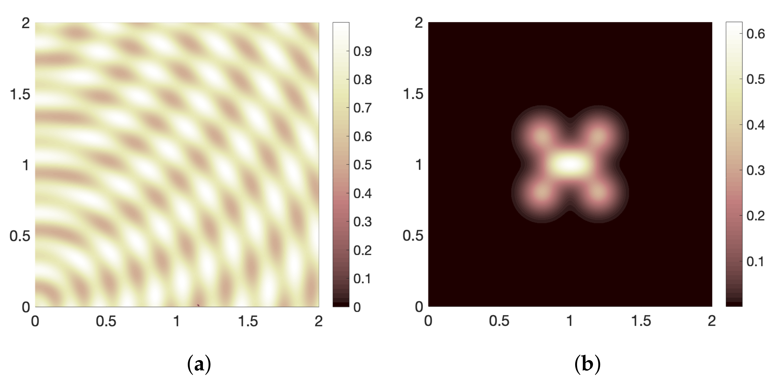
The initial spatial distribution of the host cells is supposed to be localised naturally everywhere (heterogeneous) in the computational domain = [ 0 , 2 ] × [ 0 , 2 ] (see Figure 1a), namely:
h ( 0 , x ) = 3 4 + s i n ( 5 π x 2 ) + s i n ( 5 π ( 1 , 0 ) x 2 ) 8 , x .
Regarding the initial spatial distribution of SARS-CoV-2 particles, we assume initially the presence of the virus takes place within at multiple sites near by high concentrations of the initial spatial distribution of target cells as shown in Figure 1b, that is:
v ( 0 , x ) = i , j { 0 , ± 0.2 , ± 0.4 } k c e x p ( k w x ( 1 + i , 1 + j ) 2 2 Δ x Δ y ) φ ( x ) , x ,
where φ ( x ) is a smooth function used to approximate values to zero outside the ball B ( ( 1 + i , 1 + j ) , 0.25 ) , while k c and k w are positive parameters used to control the amount of viral concentration and viral spatial distribution width in the maximal reference region. Moreover, since we suppose at t = 0 no pre-existing infected cells, chemokines, the effector T cells, the regulatory T cells, B cells and antibodies, hence we have the following initial conditions:
i ( 0 , x ) = 0 , x , c ( 0 , x ) = 0 , x , f ( 0 , x ) = 0 , x , r ( 0 , x ) = 0 , x , β ( 0 , x ) = 0 , x , α ( 0 , x ) = 0 , x .
Finally, our system is assumed to be solved within a fixed computational domain = [ 0 , 2 ] × [ 0 , 2 ] with no molecular transport across the domain boundary , thus we impose Neumann zero flux boundary conditions for all components, namely:
k , ν = 0 k { h , i , v , c , f , r , β , α } on ( 0 , ) × ,
where ν indicates the outward unit normal for vector field to the computational domain boundary .

3.3. Computational Implementation

For computational purposes, we set the maximum spatial domain to be considered within a square region, namely, : = [ 0 , 2 ] × [ 0 , 2 ] which equals to a physical domain of length [ 0 , 0.1 ] × [ 0 , 0.1 ] cm . We discretise R 2 by an equal (uniform) spatial mesh in both directions of length Δ x = Δ y : = 1 × 10 2 which is equivalent to 1 × 10 3 cm in a physical dimensional domain. For time, we discretise the time interval [ t 0 , t 0 + Δ t ] by a uniformly time step of size δ t ^ : = Δ t N with time nodes N + 1 > 1 . Thus, at any spatially discretized point ( p Δ x , q Δ y ) , p , q : = 0 , . . . and at any discretized time node t n = t 0 + n δ t ^ , n = 0 , 1 , . . . , N , we denote the concentrations for all components of the system (8) by M k ( t n , ( x p , y q ) ) k { h , i , v , c , f , r , β , α } . Further, we express the spatial operators for each component of the system (8) by S k ( t n , ( x p , y q ) ) : = 2 M k ( t n , ( x p , y q ) ) and S ^ k ^ ( t n , ( x p , y q ) ) : = M k ^ ( t n , ( x p , y q ) ) k ^ { v , f , r , β } . Hence, at any discretized spatial temporal node ( t n , ( x p , y q ) ) , we approximate the diffusion terms in (8) by a central difference scheme using a fictitious grid points of the form ( M k ) p ± 1 2 , q n , ( M k ) p , q ± 1 2 n , namely:
( S k ) p , q n ( ( M k ) x ) p + 1 2 , q n ( ( M k ) x ) p 1 2 , q n Δ x + ( ( M k ) y ) p , q + 1 2 n ( ( M k ) y ) p , q 1 2 n Δ y .
Additionally, we approximate the chemotaxis terms in (8) by the following expression:
( S ^ k ^ S c ) p , q n ( M k ^ ) p + 1 2 , q n ( ( M c ) x ) p + 1 2 , q n ( M k ^ ) p 1 2 , q n ( ( M c ) x ) p 1 2 , q n Δ x + ( M k ^ ) p , q + 1 2 n ( ( M c ) y ) p , q + 1 2 , n ( M k ^ ) p , q 1 2 n ( ( M c ) y ) p , q 1 2 n Δ y ,
where
( ( M k ) x ) p + 1 2 , q n : = ( M k ) p + 1 , q n ( M k ) p , q n Δ x , ( ( M k ) x ) p 1 2 , q n : = ( M k ) p , q n ( M k ) p 1 , q n Δ x , ( ( M k ) y ) p , q + 1 2 n : = ( M k ) p , q + 1 n ( M k ) p , q n Δ x , ( ( M k ) y ) p , q 1 2 n : = ( M k ) p , q n ( M k ) p , q 1 n Δ x ,
and
( M k ^ ) p ± 1 2 , q n : = ( M k ^ ) p , q n + ( M k ^ ) p ± 1 , q n 2 , ( M k ^ ) p , q ± 1 2 n : = ( M k ^ ) p , q n + ( M k ^ ) p , q ± 1 n 2 .
For time discretisation, we use the predictor corrector method to approximate the solutions i.e., on the interval [ t n , t n + 1 ] , we predict the density for each component ( M k ) by the explicit Euler method, namely:
( M ˜ k ) p , q n + 1 = ( M k ) p , q n + δ t ( F ( h p , q n , i p , q n , v p , q n , c p , q n , f p , q n , r p , q n , β p , q n , α p , q n ) ) ,
where the function F ( · ) denotes all terms of the right hand side of the system (8) including the diffusion ( S k ) and chemotaxis ( S ^ k ^ ) operators. Then, we correct the predicted solutions via the following Trapezoidal approximation rule as well as using predict-evaluate-correct mode to obtain a better approximation of the solution, namely,
( M ^ k ) p , q n + 1 = ( M k ) p , q n + 1 2 δ t ( F ( h p , q n , i p , q n , v p , q n , c p , q n , f p , q n , r p , q n , β p , q n , α p , q n ) + F ( h ˜ p , q n , i ˜ p , q n , v ˜ p , q n , c ˜ p , q n , f ˜ p , q n , r ˜ p , q n , β ˜ p , q n , α ˜ p , q n ) ) . ( M k ) p , q n + 1 = ( M k ) p , q n + 1 2 δ t ( F ( h p , q n , i p , q n , v p , q n , c p , q n , f p , q n , r p , q n , β p , q n , α p , q n ) + F ( h ^ p , q n , i ^ p , q n , v ^ p , q n , c ^ p , q n , f ^ p , q n , r ^ p , q n , β ^ p , q n , α ^ p , q n ) ) .
Thus, following the same procedures, we obtain solutions on the computational domain for each component of (8), that is, for all ( M k ) p , q n k { h , i , v , c , f , r , β , α } .

3.4. Data Estimation

In general, parameter estimation in computational immunology is still a major problem due to either the lack of experimental data at a cellular level or the differences between results from study to study. The estimations of parameters are impacted by many factors such as cells shape, size and type, methods and laboratory equipments as well as the interpretation of the laboratory data [45,46]. However, simulations may provide an efficient manner for immunological exploration and prediction. Therefore, the model validation could be investigated without knowing the data where this common methodology is used during the exploratory steps [47]. Although the shortage of experimental studies about COVID-19, we select a list of values for model parameters to simulate the baseline case for which they are considered as a starting point for the numerical investigation. The baseline values (as shown in Table 1) have been built on clinical and mathematical results, namely [19,22,26,27,34,44]. We estimate diffusion rates building on the size and the shape of cells and particles as detailed in [44] with taking into consideration the unit of diffusion as the area per unit time where we mainly use centimeters as units for measuring length and seconds for time. Further, we pick out the other motility rates and chemotaxis coefficients for immune system components based on biological ranges specified in [34].
For production and decay rates, we select the baseline values depending on few recent mathematical studies [22,26,27] used temporal (within host) modelling approaches for COVID-19. However, most of these data have been collected from previous studies for similar infectious diseases such as dengue infection, HIV infection and AIDS. Therefore, we still face a lack of experimental data for infection with SARS-CoV-2, especially at the cellular scale.

4. A Comparison of Computational and Clinical Results

In this section, we aim to investigate numerically the dynamics of host cells h ( t , x ) , infected cells i ( t , x ) , SARS-CoV-2 particles v ( t , x ) , chemokines c ( t , x ) , the effector T cells f ( t , x ) , the regulatory T cells r ( t , x ) , B-lymphocytes cells β ( t , x ) and antibodies α ( t , x ) . These dynamics are computed at each discretized spatio-temporal node ( t n , ( x p , y q ) ) within a computational domain of size = [ 0 , 2 ] × [ 0 , 2 ] which equals to a physical domain [ 0 , 0.1 ] × [ 0 , 0.1 ] cm . For time steps, we run the numerical simulation for 120 stages (120,000 Δ t ), which equals approximately 333.34 h. However, SARS-CoV-2 particles may remain in the body for more than 60 days or sometimes reaching 150 days as discussed in [5,19,48], which corresponds to 259,200 Δ t 650,000 Δ t (in non-dimensionalised time step). Moreover, we choose the following initial values for the variables those defined in Section 3.1 based on some biological and mathematical observations [19,20,27], h 0 = 4 × 10 5 , i 0 = 3 × 10 4 , v 0 = 357 × 10 4 , c 0 = 0.1 , f 0 = 500 , r 0 = 150 , β 0 = 100 , α 0 = 0.1 . In the following context, we discuss the validation of the suggested model (8) with regards to experimental observations in terms of the viral load of SARS-CoV-2 during time. As mentioned in Section 1, there are a bunch of studies that discuss a within host modeling of SARS-CoV-2 interactions with immune system components, but these studies consider only the temporal dynamics of this interaction. Hence, there is a lack of both computational and experimental data for the spatial distribution of SARS-CoV-2 within the cellular scale. However, we still wish that our suggested spatio-temporal model (8) will stimulate experimental works to validate our numerical findings.
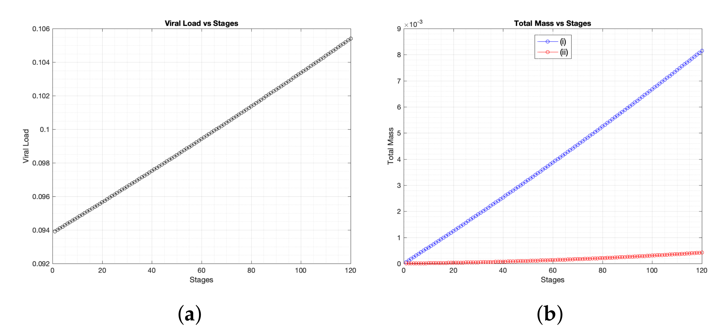
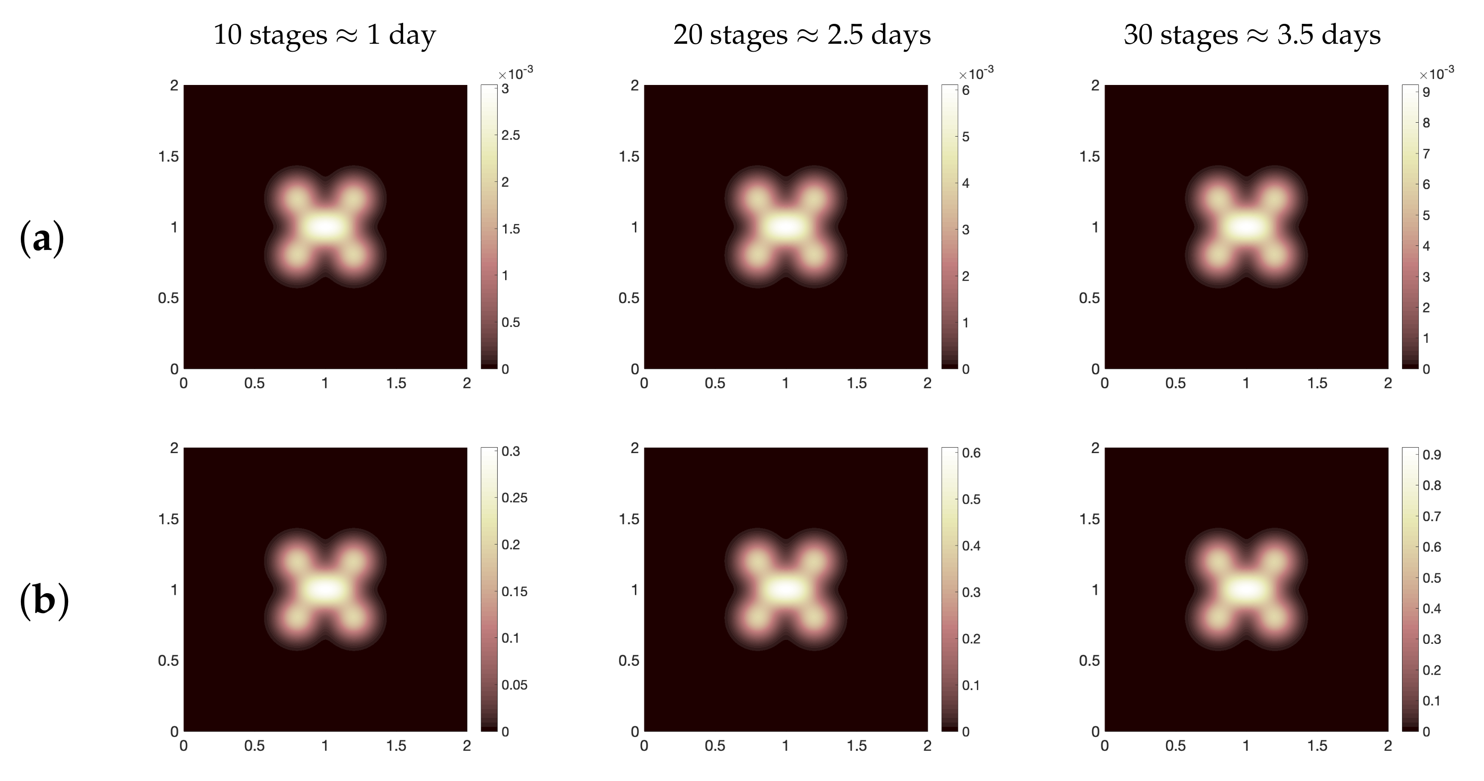
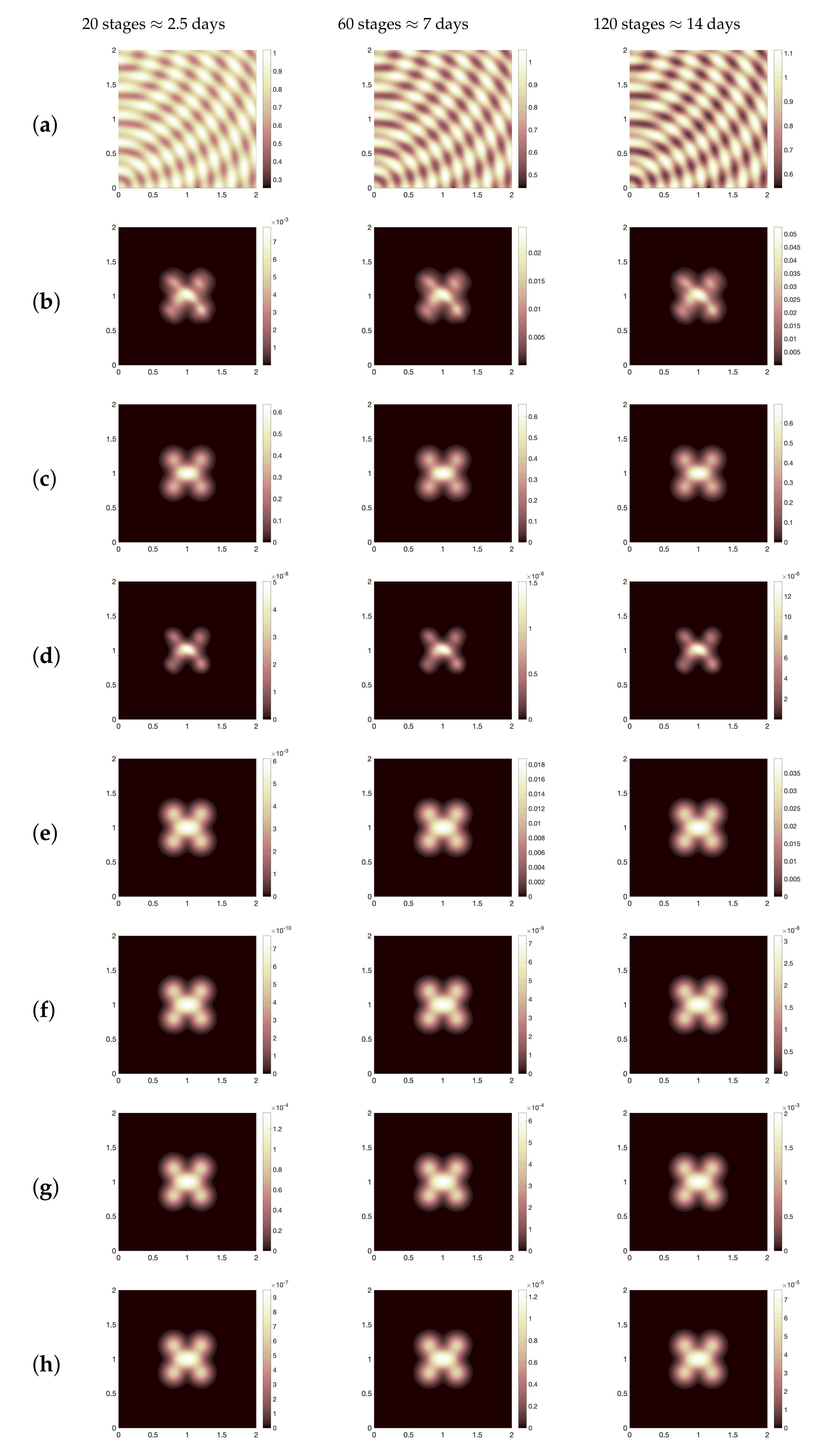
Now, in order to check the validation of our modeling assumptions, we first select a list of values for the model parameters as presented in Table 1 which mainly based on the following published studies [19,22,26,27,34,44]. Using this baseline values, we show the spatial distribution for all dynamics as illustrated in Figure 2 where we present (for three different time periods, namely, ≈2.5 days, 7 days, 14 days): healthy cells (a), infected cells (b), SARS-CoV-2 particles (c), chemokines (d), the effector T cells (e), the regulatory T cells (f), B-lymphocytes cells (g) and antibodies (h). It is obvious to see that the spatial distribution of immune components follows the same distribution patterns of virus. Moreover, for the parameter regimes that we have selected as a starting point for the computational investigation, we find that the total viral load of SARS-CoV-2 increases since day one of infection. This increase of virus occurs due to the slow growth of T and B cells over time (see Figure 3a,b). However, comparing our computational result with patients data for the whole clinical course that have been considered in [49], we conclude the following, in the clinical data, the average virus load in swab test was about 3.44 × 10 5 copies per mL on the day 5 which equals to 9.64 × 10 2 in non-dimensional values, while numerically, the viral load on the day 5 is almost equal to 9.58 × 10 2 , that is, 3.42 × 10 5 (see Figure 4a–i). Nevertheless, the baseline scenario of the numerical simulation represents a failure of immune responses to infection with SARS-CoV-2 because it is clearly to see that the density of infected cells increases from day one of infection until 14 days. This immunity failure probably occurred due to the late response of T cells (especially for asymptomatic cases) as presented in Figure 5 where we compare the effector T cells evolution at early time stages for two cases of immune responses to SARS-CoV-2, namely, baseline scenario and a better case of immunity responses (it will be explained in detail in the next context). Further, the slow response of T cells is negatively reflected on B cells growth and the activation process of antibodies.
In the following, we investigate the impact of variation of parameters on the level of SARS-CoV-2 viral load over a certain period of time. To that end, we first denote the virus domain * ( t 0 ) to be a sub-domain located entirely within our computational domain, that is, * ( t 0 ) ( t 0 ) . Then, we define a new function ψ ( · , · ) which enables increasing or decreasing the level of all system components exclusively at each grid point containing a non-zero solution of virus i.e., at every ( v ) p , q n | v 0 , p , q * ( t 0 ) . Accordingly, ψ ( · , · ) is expressed as follows:
ψ ± ( p , q ) : = ζ if ( x p , y q ) * ( t 0 ) ¯ , 1 if ( x p , y q ) * ( t 0 ) ¯ ,
where * ( t 0 ) ¯ is the topological closure of * ( t 0 ) and the percentage variable ζ is given by the following choices:
ζ : = { 100 % , 150 % , 200 % } .
Thus, the system (8) can be rewritten in the following form:
h t = D h 2 h + μ h h ( 1 h ) δ 11 h , i t = D i 2 i + ψ μ i h v δ 21 i f δ 22 i , v t = D v 2 v χ v · ( v c ) + ψ μ v i δ 31 α v δ 32 v , c t = D c 2 c + μ c i f δ 41 c , f t = D f 2 f χ f · ( f c ) + ψ + μ f v v + k f δ 51 r f δ 52 f , r t = D r 2 r χ r · ( r c ) + ψ μ r f f + k r δ 61 r , β t = D β 2 β χ β · ( β c ) + ψ + μ β v v + k β + ψ + μ β ˜ f δ 71 β , α t = D α 2 α + ψ + μ α β δ 81 α .
Just to note that the system (12) is only computed by using one of the functions ( ψ + , ψ ) , for example, if we plug the function ( ψ + ) into system (12), the other function ( ψ ) will be implemented as a matrix of ones during computations. Based on that, we can divide the parameters into two main groups, namely, (A) parameters that, if increased, would decrease the overall viral load over time (motivation occurs at a rate ψ + ) and (B) parameters that, if increased, would increase the level of viral load (that occurs at a rate ψ ).
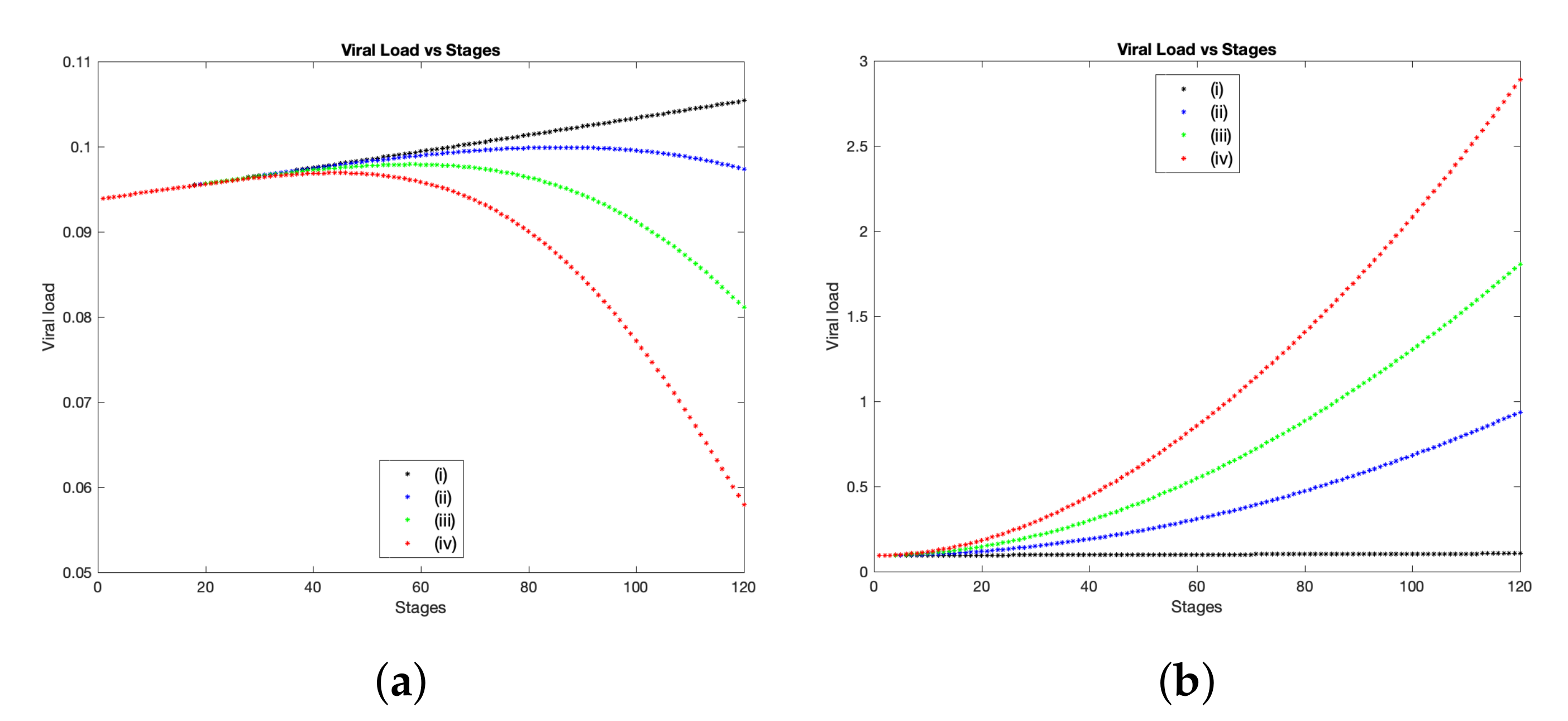
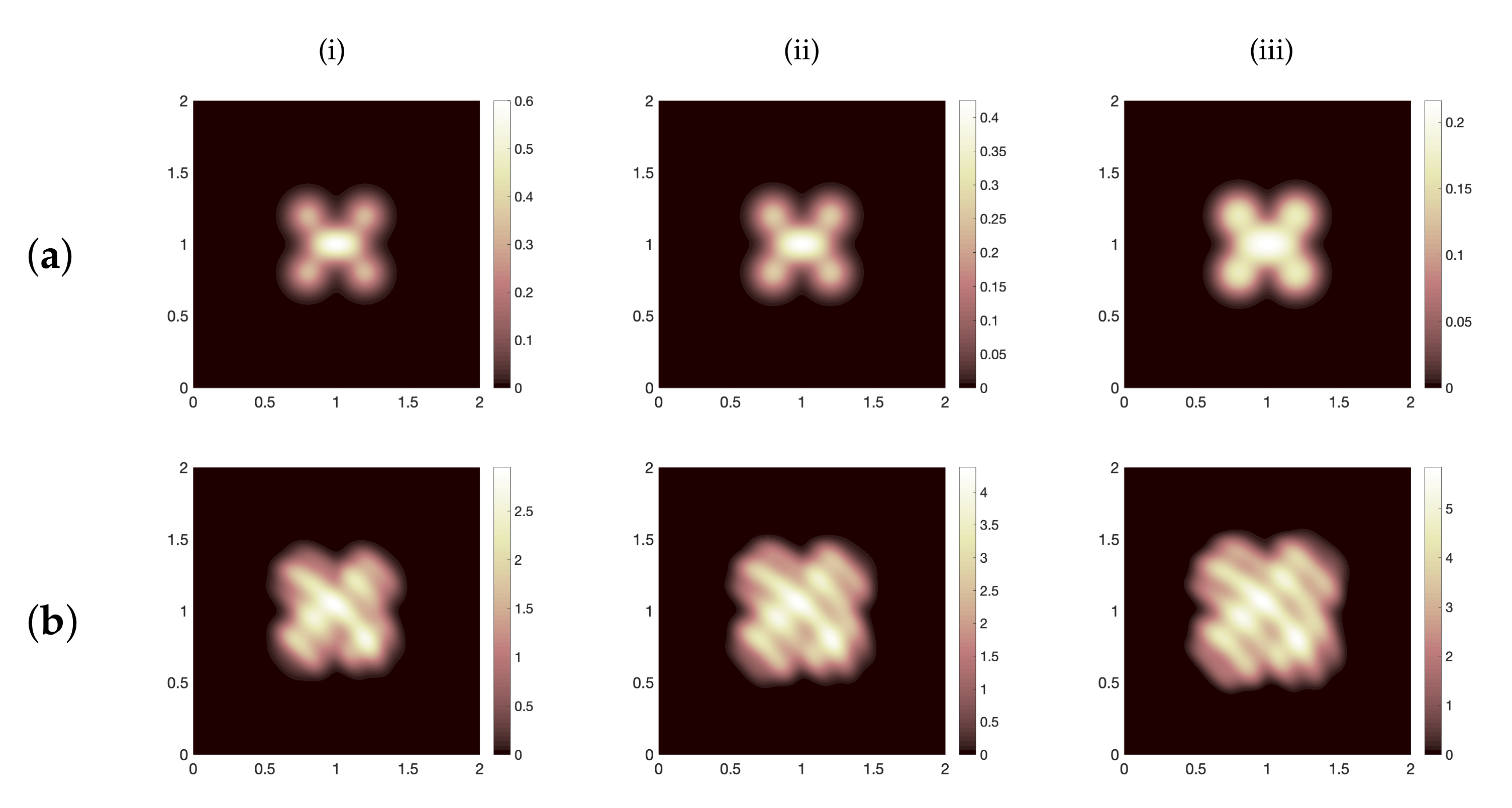
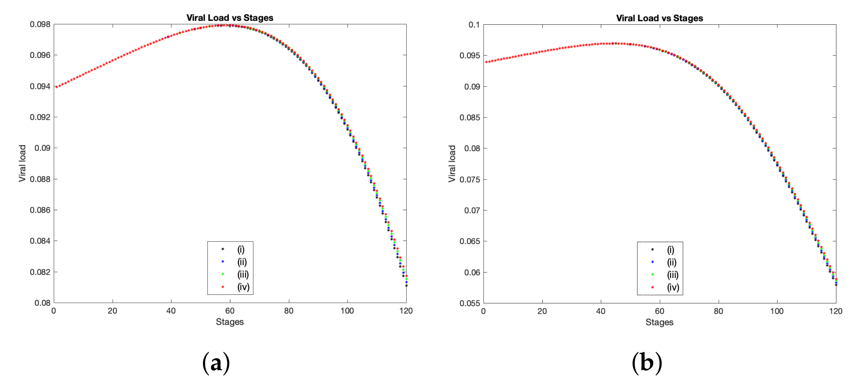
Now, we start the sensitivity analysis using the percentage variable ζ to explore the impact of parameters defined in group (A) upon the overall result. In general, increasing this group of parameters leads to a proportional decay on the overall viral load of SARS-CoV-2 over time. In other words, increasing the percentage variable ( ζ ) brings a clear influence towards controlling the infection with SARS-CoV-2. This result is obvious in Figure 4a, where we show the total viral load of SARS-CoV-2 over 120 stages which corresponds to approximately 14 days. The black curve represents the basic scenario using the baseline values presented in Table 1, while the blue, green and red curves illustrate the same case, but with employing the percentage variable ζ : = 100 % , ζ : = 150 % and ζ : = 200 % respectively. The experimental study [41] shows the amount of viral load of SARS-CoV-2 for more than 80 patients over 12 to 15 days. The peak of viral load occurs between 5 to 6 or 7 days post symptom onset. However, the median time of symptom onset was varying from 2 to 7 days according to [22]. Here, we mainly focus on two patients from Beijing where their daily clinical samples were collected from throat swabs, urine, stool and sputum as presented in [41]. The first patient has a peak of viral load in throat swap in almost 7 days, while the second patient has that peak by the day 5. Hence, in order to compare our computational findings with the above samples results, we find that in the case when ζ : = 200 % , simulations show that the peak of viral load takes place at stage 43 which corresponds to the day 5 where this result coincides with clinical samples collected from the throat swabs for the second patient (see Figure 4a(iv)). Moreover, the viral load copies (per mL) at the peak point is ranging from 10 4 to 10 8 as collected from clinical data [41,49], while in our numerical results, when ζ : = 200 % , the viral load (on the day 5) is equal to 9.69 × 10 2 copies per ml (≈ 3.46 × 10 5 —dimensional value). However, in the case when ζ : = 100 % , 150 % , the peak of viral load appears at stage 80 and 54 (which corresponds to the day 9.25 and the day 6.25) with concentrations of 9.99 × 10 2 and 9.79 × 10 2 copies per ml (which equals to 3.565 × 10 5 and 3.495 × 10 5 ), respectively. Consequently, for both cases of ζ : = 150 % , 200 % , the viral load tends to peak within the same time range compared to data collected from clinical trials. Further, in Figure 6a, we show the spatial distribution of virus particles at the final stage (14 days) for the three cases of ζ , namely, ζ : = (i) 100 % , (ii) 150 % and (iii) 200 % . Thus, this result confirms that increasing the parameter values specified in group (A) leads to a better scenario with regards to infection with SARS-CoV-2.
On other hand, to observe the impact of the parameters defined in group (B) on the overall virus spatial expansion and the total viral load during interactions between virus and immune components, we first let ψ ( p , q ) be denoted by the formula defined in (10), while substituting the function ψ + ( p , q ) by one into model (12) p , q * ( t 0 ) . Then, using parameters values presented in Table 1 and changing ζ by percentages determined in (11), we show a comparison of viral load of SARS-CoV-2 for the above scenario starting from 2.78 h (stage 1) to 14 days (stage 120). Numerically, we obtain a higher viral load and more expansion of spatial distribution on the computational domain whenever ζ is increased (see Figure 4b and Figure 6b). This undesirable growth of virus can be explained by the fact that both rates of infection and viral replication have been considered within group (B), therefore increasing these rates by ψ will mostly cause more viral load over time. Following similar scenarios from clinical findings for died patients as presented in [41], the viral load on the day 8 was at least equal to 10 6 for nasal swab and 1.34 × 10 11 for sputum sample. Hence, in a comparison to our simulations, the viral load on the day 8 (at stage 69) is greater than 10 6 (copies per mL) in dimensional values for all cases of ζ , namely, when ζ : = 100 % : viral load is 0.376 (non-dim) which equals to ≈ 1.34 × 10 6 (dim); when ζ : = 150 % : viral load is 0.687 (non-dim) ≈ 2.45 × 10 6 (dim); when ζ : = 200 % : viral load is 1.08 (non-dim) ≈ 3.85 × 10 6 (dim). Thus, rising the parameters defined in group (B) drives to a serious situation of infection with SARS-CoV-2.
Another factor that affects SARS-CoV-2 infection is the variation of random motility rates for cells, virus and chemokines on the spatial domain. To check this, we decide to duplicate, triplicate and quadruplicate the diffusion rates for all system components using best outcomes in regards to viral load control, namely, substituting the function ψ + as defined in (10) into system (12) with ζ : = { 150 % , 200 % } , while ψ : = 1 (these cases are illustrated in Figure 4a(iii,iv)). Accordingly, in Figure 7 we show the evolution of viral load of SARS-CoV-2 over 14 days using three values of random motility rates for all system components i.e., 2 D k , 3 D k , 4 D k k { h , i , v , c , f , r , β , α } where Figure 7a represents the viral load evolution in the case when ζ : = { 150 % } , while Figure 7b shows the same case but when ζ : = { 200 % } . In general, numerical results show that there is a viral load growth whenever diffusion coefficients are increased. This result could be explained as follows, fast spatial diffusion of system components (especially infected cells and virus particles) within the tissue (our computational domain ) could expand the area of the dynamical interaction as well as transfer the virus to respiratory system which that may drive to have a late and a huge immune responses causing the cytokine release syndrome and leading to serious damage of vital organs and death in the worst cases [8,11,16].

5. Discussion

In contrast to the temporal mathematical models (either between-host or within-host models) as presented in [21,22,23,24,25,26], we here suggested a new spatio-temporal (within-host) mathematical model to describe the interactions at the cellular scale between healthy cells, viral infected cells, SARS-CoV-2 particles and the main parts of immune system, namely, effector and regulatory T cells, B-lymphocytes cells and antibodies in the presence of chemokines concentration. Modeling assumptions and settings were carefully selected building on recent biomedical and mathematical studies as detailed in Section 2. The numerical simulations provided reasonable outcomes for the within-host infection scenario which harmonized with data collected from clinical samples. However, we have faced many challenges regarding data availability as well as investigating the model outputs in a comparison with observations collected from clinical studies.
To investigate the model validation, we have improved a part of the computational framework introduced in [50] and then extended in [39]. Besides the implementation process of the finite difference method including approximations of the diffusion and chemotaxis terms, we have inserted additional strategies involving predict-evaluate-correct mode (see Section 3.3) with taking into account a multi-site of infection on the computational domain and assuming a heterogeneous initial condition for host cells (see Section 3.2) as well as applying certain conditions such as increasing the density of system components exclusively on the virus domain * ( t 0 ) . We investigated numerically multiple scenarios compared to the baseline parameter regimes presented in Table 1 where the majority of these values are selected from [19,22,26,27,34,44]. However, simulation results using these values showed a failure case of immune responses to SARS-CoV-2 as presented in Figure 4a(i). Hence, we decided to define the functions ψ ± ( · , · ) (which exercise their role exclusively at * ( t 0 ) ( t 0 ) ) in order to study the sensitivity of solutions using three choices of the percentage variable ( ζ ) . Based on that, we conclude the following, increasing the production rates of some immune components, namely, ( μ f , μ β , μ β ˜ , μ α ) by a size of ψ + ( · , · ) leads to a clear decay in the total viral load during time, conversely, rising the parameters ( μ i , μ v , μ r ) by a quantity of ψ ( · , · ) encouraged the viral replication and reduced T cells production which in turn caused a growth of the total viral load. Additionally, in the case when ψ + ( · , · ) is considered into model (12), we have found that staying at the peak of viral load differs as the percentage variable changes, for example, when ζ : = 100 % , the viral load reaches the peak after passing 9.25 days and remains on peak for another 36 h and 6.6 min, then decreases on the day 10.5 (for the other cases of ( ζ ) , see Table 2). Furthermore, increasing the motility rates for system components would play a central role on the growth of the viral load over time. In general, for all cases of ( ζ ), our numerical results almost fit clinical outcomes for some patients data collected from [41,49] in terms of the amount of viral load on peaks (in dimensional values—copies per ml) as well as the time of the peak of viral load.
In this work, we have mainly presented a mathematical framework for modeling the immune responses to SARS-CoV-2 using a system of partial differential equations. We have developed a computational approach in order to simulate some scenarios of viral infection at a cellular level. Numerically, we have obtained a better control of SARS-CoV-2 infection in the case when the production level of T cells increases, and B cells and antibodies are exclusively in the spatial domain of the virus. From an immunological perspective, the ability to generate a strong immune response varies between people due to multiple factors. Therefore, we hope that the assumptions formulated in this work will stimulate suitable experimental studies that would investigate the production level of immune components at the infection site. However, in the future, we aim to provide further insight into the other factors such as the resulting pathological damages caused by either virus interactions with surrounding components or the cytokine storm caused by immune system. Moreover, questions regarding the qualitative behavior of the model, the local existence and uniqueness remain an open problem which could be investigated in a later work. Further, topics of COVID-19 are one of the most important research priorities nowadays; therefore, mathematical works should keep track of these efforts which require further improvement and future work. Thus, the proposed modeling framework and the computational technique can be extended to follow new findings from the forthcoming experimental studies.
Funding

This research received no external funding.

Institutional Review Board Statement

Not applicable.

Informed Consent Statement

Not applicable.

Data Availability Statement

Not applicable.

Conflicts of Interest

The author declares no conflict of interest.

References

  1. Yao, Y.; Chen, W.; Wu, X.; Shen, L.; Shen, L.; Fu, Y.; Yang, Q.; Yao, M.; Zhou, J.; Zhou, H. Clinical characteristics of COVID-19 patients in three consecutive generations of spread in Zhejiang, China. Clin. Microbiol. Infect. 2020, 26, 1380–1385. [Google Scholar] [CrossRef] [PubMed]
  2. Cucinotta, D.; Vanelli, M. WHO Declares COVID-19 a Pandemic. Acta Biomed. 2020, 91, 157–160. [Google Scholar] [PubMed]
  3. Cheng, C.; Zhang, D.; Dang, D.; Geng, J.; Zhu, P.; Yuan, M.; Liang, R.; Yang, H.; Jin, Y.; Xie, J.; et al. The incubation period of COVID-19: A global meta-analysis of 53 studies and a Chinese observation study of 11,545 patients. Infect. Dis. Poverty 2021, 10, 119. [Google Scholar] [CrossRef]
  4. Ren, X.; Wen, W.; Fan, X.; Hou, W.; Su, B.; Cai, P.; Li, J.; Liu, Y.; Tang, F.; Zhang, F.; et al. COVID-19 immune features revealed by a large-scale single-cell transcriptome atlas. Cell 2021, 184, 1895–1913. [Google Scholar] [CrossRef] [PubMed]
  5. Zapor, M. Persistent detection and infectious potential of SARS-CoV-2 virus in clinical specimens from COVID-19 patients. Viruses 2020, 12, 1384. [Google Scholar] [CrossRef] [PubMed]
  6. Sherina, N.; Piralla, A.; Du, L.; Wan, H.; Kumagai-Braesch, M.; Andréll, J.; Braesch-Andersen, S.; Cassaniti, I.; Percivalle, E.; Sarasini, A.; et al. Persistence of SARS-CoV-2-specific B and T cell responses in convalescent COVID-19 patients 6–8 months after the infection. Med 2021, 2, 281–295. [Google Scholar] [CrossRef]
  7. Kos, I.; Balensiefer, B.; Lesan, V.; Kaddu-Mulindwa, D.; Thurner, L.; Christofyllakis, K.; Bittenbring, J.T.; Ahlgrimm, M.; Seiffert, M.; Wagenpfeil, S.; et al. Increased B-cell activity with consumption of activated monocytes in severe COVID-19 patients. Eur. J. Immunol. 2021, 51, 1449–1460. [Google Scholar] [CrossRef]
  8. Shah, V.K.; Firmal, P.; Alam, A.; Ganguly, D.; Chattopadhyay, S. Overview of immune response during SARS-CoV-2 infection: Lessons from the past. Front. Immunol. 2020, 11, 1949. [Google Scholar] [CrossRef]
  9. Nowak, M.A.; May, R.M. Virus Dynamics: Mathematical Principles of Immunology and Virology; Oxford University Press: Oxford, UK, 2000. [Google Scholar]
  10. Wang, C.; Zhou, X.; Wang, M.; Chen, X. The impact of SARS-CoV-2 on the human immune system and microbiome. Infect. Microbes Dis. 2020, 3, 14–21. [Google Scholar] [CrossRef]
  11. Cevik, M.; Kuppalli, K.; Kindrachuk, J.; Peiris, M. Virology, transmission, and pathogenesis of SARS-CoV-2. BMJ 2020, 371, m3862. [Google Scholar] [CrossRef]
  12. Janeway, C.A., Jr.; Travers, P.; Walport, M. Immunobiology: The Immune System in Health and Disease, 5th ed.; Garland Science: New York, NY, USA, 2001; Volume 9. [Google Scholar]
  13. Lipsitch, M.; Grad, Y.H.; Sette, A.; Crotty, S. Cross-reactive memory T cells and herd immunity to SARS-CoV-2. Nat. Rev. Immunol. 2020, 20, 709–713. [Google Scholar] [CrossRef]
  14. Quast, I.; Tarlinton, D. B cell memory: Understanding COVID-19. Immunity 2021, 54, 205–210. [Google Scholar] [CrossRef]
  15. French, M.A.; Moodley, Y. The role of SARS-CoV-2 antibodies in COVID-19: Healing in most, harm at times. Respirology 2020, 25, 680–682. [Google Scholar] [CrossRef] [PubMed]
  16. Zhang, Y.; Geng, X.; Tan, Y.; Li, Q.; Xu, C.; Xu, J.; Hao, L.; Zeng, Z.; Luo, X. New understanding of the damage of SARS-CoV-2 infection outside the respiratory system. Biomed. Pharmacother. 2020, 127, 110195. [Google Scholar] [CrossRef]
  17. Macnamara, C.; Eftimie, R. Memory versus effector immune responses in oncolytic virotherapies. J. Theor. Biol. 2015, 377, 1–9. [Google Scholar] [CrossRef] [PubMed] [Green Version]
  18. Hancioglu, B.; Swigon, D.; Clermont, G. A dynamical model of human immune response to influenza A virus infection. J. Theor. Biol. 2007, 246, 70–86. [Google Scholar] [CrossRef]
  19. Sasmal, S.K.; Dong, Y.; Takeuchi, Y. Mathematical modeling on T-cell mediated adaptive immunity in primary dengue infections. J. Theor. Biol. 2017, 429, 229–240. [Google Scholar] [CrossRef] [PubMed]
  20. Nikin-Beers, R.; Ciupe, S.M. The role of antibody in enhancing dengue virus infection. Math. Biosci. 2015, 263, 83–92. [Google Scholar] [CrossRef]
  21. Batista, B.; Dickenson, D.; Gurski, K.; Kebe, M.; Rankin, N. Minimizing disease spread on a quarantined cruise ship: A model of COVID-19 with asymptomatic infections. Math. Biosci. 2020, 329, 108442. [Google Scholar] [CrossRef] [PubMed]
  22. Hernandez-Vargas, E.A.; Velasco-Hernandez, J.X. In-host mathematical modelling of COVID-19 in humans. Annu. Rev. Control 2020, 50, 448–456. [Google Scholar] [CrossRef]
  23. Jiang, S.; Li, Q.; Li, C.; Liu, S.; He, X.; Wang, T.; Li, H.; Corpe, C.; Zhang, X.; Xu, J.; et al. Mathematical models for devising the optimal SARS-CoV-2 strategy for eradication in China, South Korea, and Italy. J. Transl. Med. 2020, 18, 345. [Google Scholar] [CrossRef]
  24. Gonzalez-Parra, G.; Martínez-Rodríguez, D.; Villanueva-Micó, R.J. Impact of a new SARS-CoV-2 variant on the population: A mathematical modeling approach. Math. Comput. Appl. 2021, 26, 25. [Google Scholar] [CrossRef]
  25. Gonzalez-Parra, G.; Arenas, A.J. Nonlinear dynamics of the introduction of a new SARS-CoV-2 variant with different infectiousness. Mathematics 2021, 9, 1564. [Google Scholar] [CrossRef]
  26. Sadria, M.; Layton, A.T. Modeling within-host SARS-CoV-2 infection dynamics and potential treatments. Viruses 2021, 13, 1141. [Google Scholar] [CrossRef]
  27. Ghostine, R.; Gharamti, M.; Hassrouny, S.; Hoteit, I. Mathematical modeling of immune responses against SARS-CoV-2 using an ensemble kalman filter. Mathematics 2021, 9, 2427. [Google Scholar] [CrossRef]
  28. Boianelli, A.; Nguyen, V.K.; Ebensen, T.; Schulze, K.; Wilk, E.; Sharma, N.; Stegemann-Koniszewski, S.; Bruder, D.; Toapanta, F.R.; Guzmán, C.A.; et al. Modeling influenza virus infection: A roadmap for influenza research. Viruses 2015, 7, 5274–5304. [Google Scholar] [CrossRef] [PubMed] [Green Version]
  29. Marchuk, G.; Petrov, R.; Romanyukha, A.; Bocharov, G. Mathematical model of antiviral immune response. I. Data analysis, generalized picture construction and parameters evaluation for hepatitis B. J. Theor. Biol. 1991, 151, 1–40. [Google Scholar] [CrossRef]
  30. Dowling, M.R.; Kan, A.; Heinzel, S.; Marchingo, J.M.; Hodgkin, P.D.; Hawkins, E.D. Regulatory T cells suppress effector T cell proliferation by limiting division destiny. Front. Immunol. 2018, 9, 2461. [Google Scholar] [CrossRef]
  31. Sanderson, C.M.; Way, M.; Smith, G.L. Virus-induced cell motility. J. Virol. 1998, 72, 1235–1243. [Google Scholar] [CrossRef] [Green Version]
  32. Knodel, M.M.; Targett-Adams, P.; Grillo, A.; Herrmann, E.; Wittum, G. Advanced hepatitis C virus replication PDE models within a realistic intracellular geometric environment. Int. J. Environ. Res. Public Health 2019, 16, 513. [Google Scholar] [CrossRef] [PubMed] [Green Version]
  33. Krummel, M.F.; Bartumeus, F.; Gérard, A. T cell migration, search strategies and mechanisms. Nat. Rev. Immunol. 2016, 16, 193–201. [Google Scholar] [CrossRef] [Green Version]
  34. Su, B.; Zhou, W.; Dorman, K.; Jones, D. Mathematical modelling of immune response in tissues. Comput. Math. Methods Med. 2009, 10, 9–38. [Google Scholar] [CrossRef] [Green Version]
  35. Almocera, A.E.S.; Nguyen, V.K.; Hernandez-Vargas, E.A. Multiscale model within-host and between-host for viral infectious diseases. J. Math. Biol. 2018, 77, 1035–1057. [Google Scholar] [CrossRef] [PubMed]
  36. Shereen, M.A.; Khan, S.; Kazmi, A.; Bashir, N.; Siddique, R. COVID-19 infection: Emergence, transmission, and characteristics of human coronaviruses. J. Adv. Res. 2020, 24, 91–98. [Google Scholar] [CrossRef]
  37. Okubo, A. Diffusion and Ecological Problems: Mathematical Models; Springer: Berlin/Heidelberg, Germany, 1980. [Google Scholar]
  38. Chaplain, M.A.J.; Lolas, G. Mathematical modelling of cancer cell invasion of tissue: The role of the urokinase plasminogen activation system. Math. Mod. Meth. Appl. Sci. 2005, 15, 1685–1734. [Google Scholar] [CrossRef] [Green Version]
  39. Alzahrani, T.; Eftimie, R.; Trucu, D. Multiscale modelling of cancer response to oncolytic viral therapy. Math. Biosci. 2019, 310, 76–95. [Google Scholar] [CrossRef] [Green Version]
  40. Matzavinos, A.; Chaplain, M.A.J.; Kuznetsov, V.A. Mathematical modelling of the spatio-temporal response of cytotoxic T-lymphocytes to a solid tumour. Math. Med. Biol. 2004, 21, 1–34. [Google Scholar] [CrossRef]
  41. Pan, Y.; Zhang, D.; Yang, P.; Poon, L.L.M.; Wang, Q. Viral load of SARS-CoV-2 in clinical samples. Lancet Infect Dis. 2020, 20, 411–412. [Google Scholar] [CrossRef]
  42. Zheng, S.; Fan, J.; Yu, F.; Feng, B.; Lou, B.; Zou, Q.; Xie, G.; Lin, S.; Wang, R.; Yang, X.; et al. Viral load dynamics and disease severity in patients infected with SARS-CoV-2 in Zhejiang province, China, January-March 2020: Retrospective cohort study. BMJ 2020, 369, m1443. [Google Scholar] [CrossRef] [Green Version]
  43. Borish, L.C.; Steinke, J.W. 2. Cytokines and chemokines. J. Allergy Clin. Immunol. 2003, 111, S460–S475. [Google Scholar] [CrossRef] [PubMed]
  44. Bray, D. Cell Movements from Molecules to Motility; Garland Science: New York, NY, USA, 2000. [Google Scholar]
  45. Gadhamsetty, S.; Beltman, J.B.; de Boer, R.J. What do mathematical models tell us about killing rates during HIV-1 infection? Immunol. Lett. 2015, 168, 1–6. [Google Scholar] [CrossRef] [PubMed] [Green Version]
  46. De Boer, R.J.; Perelson, A.S. Quantifying T lymphocyte turnover. J. Theor. Biol. 2013, 327, 45–87. [Google Scholar] [CrossRef] [Green Version]
  47. Handel, A.; La Gruta, N.L.; Thomas, P.G. Simulation modelling for immunologists. Nat. Rev. Immunol. 2020, 20, 186–195. [Google Scholar] [CrossRef] [PubMed]
  48. Gabbrielli, M.; Gandolfo, C.; Anichini, G.; Candelori, T.; Benvenuti, M.; Savellini, G.G.; Cusi, M.G. How long can SARS-CoV-2 persist in human corpses? Int. J. Infect. Dis. 2021, 106, 1–2. [Google Scholar] [CrossRef]
  49. Wölfel, R.; Corman, V.M.; Guggemos, W.; Seilmaier, M.; Zange, S.; Müller, M.A.; Niemeyer, D.; Jones, T.C.; Vollmar, P.; Rothe, C.; et al. Virological assessment of hospitalized patients with COVID-2019. Nature 2020, 581, 465–469. [Google Scholar] [CrossRef] [PubMed] [Green Version]
  50. Trucu, D.; Lin, P.; Chaplain, M.A.J.; Wang, Y. A multiscale moving boundary model arising in cancer invasion. Multiscale Model. Sim. 2013, 11, 309–335. [Google Scholar] [CrossRef]
Figure 1. (a) Initial condition for healthy (host) cells density and (b) Initial condition for SARS-CoV-2 density.
Mathematics 09 03274 g001
Figure 2. Spatial distribution for all dynamics in system (8) at three time stages (20, 60 and 120) using the baseline parameter values from Table 1, presenting: (a) healthy cells density, (b) infected cells density, (c) SARS-CoV-2 particles density, (d) chemokines density, (e) the effector T cells density, (f) the regulatory T cells density, (g) B-lymphocytes cells density and (h) antibodies density.
Mathematics 09 03274 g002
Figure 3. Comparison of viral load of SARS-CoV-2 and total mass of immune cells over time stages from 1 to 120 (which is equivalent to approximately 2.78 h to 14 days) for system (8) using the baseline values presented in Table 1. (a) viral load of SARS-CoV-2, (b) total mass of immune cells; (i) T cells and (ii) B cells.
Mathematics 09 03274 g003
Figure 4. Comparison of viral load of SARS-CoV-2 over time stages from 1 to 120 (which is equivalent to approximately 2.78 h to 14 days) for system (12) using the baseline values presented in Table 1 for multiple scenarios of the percentage variable ( ζ ) . (a) when ψ + is represented by (10) and ψ : = 1 , (b) when ψ is represented by (10) and ψ + : = 1 . (i) Baseline case. (ii) ζ : = 100 % . (iii) ζ : = 150 % . (iv) ζ : = 200 % .
Mathematics 09 03274 g004
Figure 5. Comparison of spatial distribution of the effector T cells evolution at early stages (10, 20, 30) (which is equivalent to approximately 1, 2.5, 3.5 days). (a) Baseline case (a failure of immune responses to SARS-CoV-2). (b) example of a better immune responses to SARS-CoV-2, namely, when ψ + is represented by (10) and ψ : = 1 ( ζ : = 100 % ).
Mathematics 09 03274 g005
Figure 6. Comparison of spatial distribution of SARS-CoV-2 evolution at the final stage (120) (which is equivalent to approximately 14 days) for system (12) using the baseline values presented in Table 1 for multiple scenarios of the percentage variable ( ζ ) . (a) when ψ + is represented by (10) and ψ : = 1 , (b) when ψ is represented by (10) and ψ + : = 1 . (i) ζ : = 100 % . (ii) ζ : = 150 % . (iii) ζ : = 200 % .
Mathematics 09 03274 g006
Figure 7. Comparison of viral load of SARS-CoV-2 over time stages from 1 to 120 (which is equivalent to approximately 2.78 h to 14 days) for three different rates of diffusion for all system components (12) using the baseline values presented in Table 1 in the case when ψ + is represented by (10) and ψ : = 1 with the following percentage variable: (a) ζ : = 150 % , (b) ζ : = 200 % . (i) D k ; (ii) 2 D k ; (iii) 3 D k ; (iv) 4 D k k { h , i , v , c , f , r , β , α } .
Mathematics 09 03274 g007
Table 1. Baseline parameters values used in numerical simulations for the spatio-temporal model of COVID-19. ( * ) indicates the modified values.
ParameterNon-Dimensional ValueDimensional ValueReferences
D h 9 × 10 4 9 × 10 10 cm 2 s 1 [44]
D i 1 × 10 4 1 × 10 10 cm 2 s 1 Est. ( D i = D h 9 )
D v 5 × 10 4 5 × 10 10 cm 2 s 1 [44]
D c 1.06 × 10 3 1.06 × 10 9 cm 2 s 1 [34]
D f 1.83 × 10 3 1.83 × 10 9 cm 2 s 1 [34]
D r 1 × 10 3 1 × 10 9 cm 2 s 1 [34]
D β 1.83 × 10 3 1.83 × 10 9 cm 2 s 1 Est. ( D β = D f )
D α 1.83 × 10 3 1.83 × 10 9 cm 2 s 1 Est. ( D α = D f )
χ v 1.67 × 10 4 1.66 × 10 9 cm 2 s 1 Est. ( χ v = χ f )
χ f 1.67 × 10 4 1.66 × 10 9 cm 2 s 1 [34]
χ r 1.67 × 10 4 1.66 × 10 9 cm 2 s 1 [34]
χ β 1.67 × 10 4 1.66 × 10 9 cm 2 s 1 Est. ( χ β = χ f )
μ h 0.462 * 0.462 × 10 1 cells mL 1 s 1 [26,27]
μ i 0.826 1.736 × 10 20 mL (RNA copies) 1 s 1 [22,27]
μ v 0.255 6 × 10 3 * s 1 [27]
μ c 0.174 0.115 × 10 4 s 1 [26,27]
μ f 0.694 0.347 × 10 1 * mL cells 1 s 1 [19,27]
μ r 0.077 0.11 × 10 2 mL cells 1 s 1 Est. ( μ r = μ f 30 )
μ β 0.0116 0.11 × 10 3 * mL cells 1 s 1 [19,27]
μ β ˜ 0.579 0.11 × 10 4 mL cells 1 s 1 Est. ( μ β ˜ = μ β 10 )
μ α 0.694 0.81 × 10 7 s 1 [19,27]
δ 11 0.0162 1.62 × 10 6 s 1 [19,27]
δ 21 0.0579 1.15 × 10 8 mL cells 1 s 1 [27]
δ 22 0.0011 1.15 × 10 7 s 1 [19,27]
δ 31 0.116 1.15 × 10 4 ml molecules 1 s 1 [19,27]
δ 32 0.04 4.05 × 10 6 * s 1 [27]
δ 41 0.0016 1.66 × 10 7 s 1 [34]
δ 51 0.52 3.47 × 10 7 mL cells 1 s 1 [34]
δ 52 0.0034 3.47 × 10 7 s 1 [34]
δ 61 0.0034 3.47 × 10 7 s 1 [34]
δ 71 0.023 2.31 × 10 6 s 1 [19,26]
δ 81 0.0081 8.1 × 10 7 s 1 [19,27]
k f 8.14 × 10 1 2.9 × 10 6 [22]
k r 5.81 × 10 3 2.9 × 10 6 [22]
k β 8.14 × 10 1 2.9 × 10 6 [22]
Δ x , Δ y 1 × 10 2 1 × 10 3 cm[44]
Δ t 1 × 10 3 10 s
Table 2. Duration and amount of viral load on the peak for each case of ζ in the case when ψ + ( · , · ) is considered into model (12) and ψ : = 1 .
CaseDuration of Viral Load PeakViral Load (Non-Dim)Viral Load (Dim)
ζ : = 100 % 36.11 h (stage 80–92) 9.99 × 10 2 3.565 × 10 5
ζ : = 150 % 25 h (stage 54–62) 9.79 × 10 2 3.495 × 10 5
ζ : = 200 % 25 h (stage 40–48) 9.69 × 10 2 3.46 × 10 5
Publisher’s Note: MDPI stays neutral with regard to jurisdictional claims in published maps and institutional affiliations.