Effect of Initial Stress on an SH Wave in a Monoclinic Layer over a Heterogeneous Monoclinic Half-Space

Abstract

Considering the propagation of an SH wave at a corrugated interface between a monoclinic layer and heterogeneous half-space in the presence of initial stress. The inhomogeneity in the half-space is the causation of an exponential function of depth. Whittaker’s function is employed to find the half-space solution. The dispersion relation has been established in closed form. The special cases are discussed, and the classical Love wave equation is one of the special cases. The influence of nonhomogeneity parameter, coupling parameter, and depth of irregularity on the phase velocity was studied.

1. Introduction

Many experimental and theoretical studies predicted that the Earth is a convoluted model in nature. Therefore, a more natural presentation of the medium through which seismic waves propagate is required. The propagation of a wave in an inhomogeneous medium is of keen interest due to the continuous variation in the elastic properties of the material. The heterogeneity in the material is produced by a change in rigidity and density. Various authors have taken various forms of the variation, like linear exponential, quadratic, etc., for simulating the variation in different geological parameters inside the Earth. Jeffrey [1] deliberated the impact of heterogeneity on the Love wave. Bullen [2] mentioned that density varies inside the Earth at different rates. Wilson [3] examined the propagation of the Rayleigh wave in a heterogeneous medium. Dhua and Chattopadhyay [4] discussed wave propagation in heterogeneous layers of the Earth. Alam et al. [5] examined the propagation of an SH-wave in an anisotropic crustal layer over a heterogeneous half-space. Taking into account the structure and characteristics of the Earth, a variety of crustal forms are possible. Crystals are solid in nature and bounded by faces or plane surfaces. The monoclinic form is one of them. It has three unequal axes, two intersecting at an oblique angle, and the third is transverse to them. Several authors worked in this direction [6,7,8,9,10,11,12].

Initial stress develops in the body due to many physical causes. The initial stress has a great impact on the rigidity of the elastic structure and produces a mechanical fault called buckling. Biot [13] firstly examined the propagation of light under initial stress. A detailed study on the propagation of Love, Rayleigh, and SH-waves in a pre-stress heterogeneous half-space was made by Chaterjee et al. [14]. Singh et al. [15] analyzed the impact of stress and irregularity on the Love wave in a heterogeneous medium. They have shown that horizontal stress has a favorable impact on the phase velocity. Abd-Alla et al. [16] discussed the impact of stress on an SV wave at the solid-liquid interface. Verma et al. [17] examined the influence of initial stress on the propagation of the Rayleigh wave in a heterogeneous medium. Khan and Afzal [18] examined the impact of initial stress on the viscoelastic liquid. They found that the reflected and refracted P wave has a maximum amplitude ratio.

Motivated in this paper by the above studies, we have considered the propagation of an SH-wave in a homogeneous monoclinic layer lying over a heterogeneous half-space. Initial stress, rigidity, and density are assumed to vary with depth. The dispersion curves are predicted by graphs for various values of non-homogeneity parameters and different sizes of irregularity.

2. Problem Formulation

Let us assume the Cartesian coordinate system; hence a wave propagating along $x$-axis and z-axis is considered vertically downward. A nonhomogeneous monoclinic layer $N_1:\left[r_1\left(x\right)-h\le z\le r_2\left(x\right)\right]$ over a heterogeneous monoclinic half-space $N_2:\left[r_2\left(x\right)\le z\le \infty \right],$ where $r_1\left(x\right)$ and $r_2\left(x\right)$ is periodic, and continuous functions of $x$ and $h$ is the thickness of the layer. The Fourier series of these functions are written as

$$r_j\left(x\right)={{\displaystyle \sum }}_{n=1}^{\infty }\left[r_n{}^j{e}^{in\alpha x}+r_{-n}{}^j{e}^{-in\alpha x}\right] ,$$

(1)

where $r_n{}^j$ and $r_{-n}{}^j$ are nth order coefficient of Fourier series expansion

$$r_{\mp n}{}^j=\left\{\begin{array}{c}\frac{a_j}{2} \mathrm{for} n=1 j=1,2,\\ \frac{S_n^j\mp Q_n^j}{2}, \mathrm{for} n=2,3,4, \dots \end{array}\right.$$

where $S_n^j$ and $Q_n^j$ are coefficient of Fourier series expansion.

Equation (1) can be explained as follow (Ref. [19])

$$r_1=a_{1}cos\alpha x , r_2=a_{2}cos\alpha x,$$

(2)

where $\alpha$ the wave is number, $a_1$ and $a_2$ are the amplitudes of the upper and wavy surface.

3. SH-Wave in Homogeneous Monoclinic Layer

We consider the equation of motion in the presence of initial stress P and magnetic field (Ref. [6]).

$${\tau }_{ij,j}-\frac{P}{2}\frac{{\partial }^2{v}_1}{\partial x^2}+{\left(\overrightarrow{J}\times \overrightarrow{B}\right)}_i={\rho }_1\frac{{\partial }^2{U}_i}{\partial t^2}, i,j=1,2,3.$$

(3)

where $U_i=\left[u_1,v_1,w_1\right]$ is the displacement vector, ${\rho }_1$ the mass density, $\overrightarrow{B}$ the magnetic induction vector, and $\overrightarrow{J}$ the electric current density.

The stress-strain relation is defined as

$${\tau }_{ij}=C_{ijkl}{e}_{kl}$$

(4)

We consider the homogeneity of the monoclinic layer as,

$$\begin{gathered} C_{12}=C_{12}, C_{11}=C_{11}, C_{13}=C_{13}, C_{25}=C_{25}, \\ {C}_{15}=C_{15}, C_{23}=C_{23} , C_{46}=C_{46}, C_{33}=C_{33,} \\ {C}_{44}=C_{44} , C_{35}=C_{35}, C_{66}=C_{66}, \\ {C}_{55}=C_{55} , C_{22}=C_{22}. \end{gathered}$$

(5)

The stress-strain relations for are given by:

$$\begin{gathered} {\tau }_{11}=C_{11}{e}_{11 }+C_{21}{e}_{22}+C_{13}{e}_{33}+C_{15}{e}_{13}, \\ {\tau }_{22}=C_{21}{e}_{11}+C_{22}{e}_{22}+C_{23}{e}_{33}+C_{25}{e}_{13}, \\ {\tau }_{33}=C_{13}{e}_{11}+C_{23}{e}_{22}+C_{33}{e}_{33}+C_{35}{e}_{13,} \\ {\tau }_{23}=C_{44}{e}_{23}+C_{46}{e}_{12}, \\ {\tau }_{13}=C_{15}{e}_{11}+C_{25}{e}_{22}+C_{35}{e}_{33}+C_{55}{e}_{13}, \\ {\tau }_{12}=C_{44}{e}_{23}+C_{66}{e}_{12}, \end{gathered}$$

(6)

where $C_{ij}=C_{ji}\left(i,j=1,2,\dots \dots ,6\right) \mathrm{are} \mathrm{elastic} \mathrm{constants} \mathrm{and}$

$$e_{ij}=\frac{1}{2}\left( \frac{\partial u_i}{\partial x_j}+\frac{\partial u_j}{\partial x_i} \right).$$

When the SH-wave is propagating in $xz$ plane, we have the following components of displacement

$$v_1=v_1\left(x,z,t\right), u_1=0=w_1.$$

(7)

Using Equation (7) into Equation (3), we have

$$\frac{\partial {\tau }_{12}}{\partial x}+\frac{\partial {\tau }_{23}}{\partial z}-\frac{P}{2}\frac{{\partial }^2{v}_1}{\partial x^2}+{\left(\overrightarrow{J}\times \overrightarrow{B}\right)}_2={\rho }_1\frac{{\partial }^2{v}_1 }{\partial t^2}.$$

(8)

Maxwell’s equations are

$$\overrightarrow{\nabla }·\overrightarrow{B}=0, \overrightarrow{\nabla }\times \overrightarrow{E}=-\frac{\partial \overrightarrow{B}}{\partial t}, \overrightarrow{ \nabla }·\overrightarrow{E}=\frac{{\rho }_e}{ϵ}, \overrightarrow{ B}={\mu }_e\overrightarrow{H,} \overrightarrow{\nabla }\times \overrightarrow{H}=\overrightarrow{J},$$

(9)

where $\overrightarrow{E}$ is the electric field, $\overrightarrow{H}$ includes both the induced and primary magnetic fields, ${\rho }_e$ is charge density, ${\mu }_e$ is permeability, $ϵ$ is the permittivity of free space, and $\sigma$ is the conduction coefficient. Then Maxwell’s stress tensor ${\left({\tau }_{\mathrm{ij}}\right)}^M$ is given by Ref. [18]

$${\left({\tau }_{\mathrm{ij}}\right)}^M={\mu }_e\left[H_i{h}_j+H_j{h}_i-H_k{h}_k{\delta }_{\mathrm{ij}}\right],$$

(10)

where $h_i=$ [$h_1,h_2,h_3]$ is the change in the magnetic field.

In the absence of displacement current Equation (9) becomes

$$\frac{{\nabla }^2\overrightarrow{H}}{{\mathsf{\sigma }\mathsf{\mu }}_e}=\left[\frac{\partial \overrightarrow{H}}{\partial t}-\overrightarrow{\nabla }\times \left(\frac{\partial \overrightarrow{U}}{\partial t}\times \overrightarrow{H}\right)\right].$$

(11)

Components form of Equation (11) is given below

$$\frac{\partial H_x}{\partial t}=\frac{1}{{\mathsf{\sigma }\mathsf{\mu }}_e}{\nabla }^2{H}_x, \frac{\partial H_y}{\partial t}=\frac{1}{{\mathsf{\sigma }\mathsf{\mu }}_e}{\nabla }^2{H}_y+\left[\frac{\partial }{\partial x}\left(H_x\frac{\partial v_1}{\partial \mathrm{t}}\right)+\frac{\partial }{\partial z}\left(H_z\frac{\partial v_1}{\partial \mathrm{t}}\right)\right], \frac{\partial H_z}{\partial t}=\frac{1}{{\mathsf{\sigma }\mathsf{\mu }}_e}{\nabla }^2{H}_y.$$

(12)

When $\mathsf{\sigma }\to \infty$ Equation (12) becomes

$$\frac{\partial H_x}{\partial t}=0=\frac{\partial H_z}{\partial t},$$

(13)

and

$$\frac{\partial H_y}{\partial t}=\left[\frac{\partial }{\partial x}\left(H_x\frac{\partial v_1}{\partial \mathrm{t}}\right)+\frac{\partial }{\partial z}\left(H_z\frac{\partial v_1}{\partial \mathrm{t}}\right)\right].$$

(14)

Equation (13) shows that $H_x$ and $H_z$ have no perturbation, but Equation (14) indicates there may be some perturbation in $H_y$. Hence there is some perturbation $h_2$ in $H_y,$ the only component of an induced magnetic field. The components of the magnetic field can be written as

$$H_{x }=H_{01}, H_y=H_{02}+h_2, H_z=H_{03}$$

(15)

Initially the $h_2$ is zero. The magnetic field is normal to the polarization of the wave, i.e., $H_{02}=0.$ The wave crosses the primary magnetic field at an angle $\Phi$.

$$\overrightarrow{H_0}=\left(H_{0}cos\Phi , 0,H_{0}sin\Phi \right),$$

$$\overrightarrow{H}=\left(H_{0}cos\Phi , h_2,H_{0}sin\Phi \right).$$

(16)

Using Equation (16) into Equation (14), one obtains

$$\frac{ \partial h_2 }{ \partial \mathrm{t}}=\frac{ \partial }{\partial \mathrm{t}}\left[H_0 cos\Phi \frac{ \partial v_1}{ \partial \mathrm{x}}+H_{0}sin\Phi \frac{ \partial v_1}{ \partial \mathrm{z}}\right].$$

(17)

Integrating on both sides, we get

$$h_2=H_{0}cos\Phi \frac{ \partial v_1}{ \partial \mathrm{x}}+H_{0}sin \Phi \frac{ \partial v_1}{ \partial \mathrm{z}}.$$

(18)

Now $\overrightarrow{J}\times \overrightarrow{B}$ becomes

$$\overrightarrow{J}\times \overrightarrow{B}={\mu }_e\left[\left(\overrightarrow{H}·\overrightarrow{\nabla }\right)\overrightarrow{H}-\frac{1}{2} \overrightarrow{\nabla }\overrightarrow{H^2}\right].$$

(19)

Putting the values of $\overrightarrow{J}\times \overrightarrow{B}$,${\tau }_{12}$ and ${\tau }_{23}$ in Equation (8), we have

$$L\frac{{\partial }^2{v}_1}{\partial x^2}+2M\frac{{\partial }^2{v}_1}{\partial x\partial z}+N\frac{{\partial }^2{v}_1}{\partial z^2}={\rho }_1\frac{{\partial }^2{v}_1 }{\partial t^2},$$

(20)

where $m=\frac{{\mu }_e{H}_0{}^2}{C_{44}},$ the coupling parameter of magnetoelastic medium,

$$L=C_{44}\left(O-\frac{p}{2C_{44}}\right), O=C_{44}\left(\frac{C_{66}}{C_{44}}+mco{s}^2\Phi \right),$$

$$M=C_{44}\left(\frac{C_{46}}{C_{44}}+mcos\Phi sin\Phi \right), N=C_{44}\left(1+msi{n}^2\Phi \right).$$

(21)

A harmonic wave traveling in the positive $x$ direction.

$$v_1=V_1\left(z\right)e^{ik\left(x-ct\right)},$$

(22)

Substituting Equation (21) into Equation (20), we have

$$\frac{d^2{V}_1\left(z\right)}{d{z}^2}+{\eta }_1\frac{d{V}_1}{dz}+{\eta }_2{V}_1\left(z\right)=0$$

(23)

where,

$${\eta }_1=2ik\frac{M}{N}, {\eta }_2=k^2\left(\frac{c^2}{c^2{}_1}-\frac{L}{N}\right), q=\frac{\sqrt{ {\eta }_1{}^2-4{\eta }_2}}{2}, c_1=\sqrt{\frac{N}{\rho }}.$$

The solution of Equation (23) is given below

$$v_1\left(z\right)=e^{-\frac{ {\eta }_1}{2}z}\left(Acosqz+Bsinqz\right)e^{ik\left(x-ct\right)}.$$

(24)

4. SH-Wave in Heterogeneous Monoclinic Half Space

Consider heterogeneous monoclinic half-space as

$$\begin{gathered} C_{21}\left(z\right)=C_{21}{e}^{vz}, C_{11}\left(z\right)=C_{11}{e}^{vz}, C_{13}\left(z\right)=C_{13}{e}^{vz}, C_{25}\left(z\right)=C_{25}{e}^{vz}, \\ {C}_{15\left(z\right)}=C_{15}{e}^{vz}, C_{23}\left(z\right)=C_{23} e^{vz}, C_{46}\left(z\right)=C_{46}{e}^{vz}, C_{33}\left(z\right)=C_{33} e^{vz}, \\ {C}_{44}\left(z\right)=C_{44}{e}^{vz}, C_{35}\left(z\right)=C_{35}{e}^{vz}, C_{66}\left(z\right)=C_{66} e^{vz}, \\ {C}_{55}\left(z\right)=C_{55}{e}^{vz}, C_{22}\left(z\right)=C_{22}{e}^{vz}, \end{gathered}$$

(25)

where $v$ is the real heterogeneous constants.

The stress-strain relations for heterogeneous medium is given as

$$\begin{gathered} {\tau }_{11}=C_{11}{e}_{11 }{e}^{vz}+C_{21}{e}_{22}{e}^{vz}+C_{13}{e}_{33}{e}^{vz}+C_{15}{e}_{13}{e}^{vz}, \\ {\tau }_{22}=C_{21}{e}_{11}{e}^{vz}+C_{22}{e}_{22}{e}^{vz}+C_{23}{e}_{33}{e}^{vz}+C_{25}{e}_{13}{e}^{vz}, \\ {\tau }_{33}=C_{13}{e}_{11}{e}^{vz}+C_{23}{e}_{22}{e}^{vz}+C_{33}{e}_{33}{e}^{vz}+C_{35}{e}_{13}{e}^{vz}, \\ {\tau }_{23}=C_{44}{e}_{23}{e}^{vz}+C_{46}{e}_{12} e^{vz} , \\ {\tau }_{13}=C_{15}{e}_{11}{e}^{vz}+C_{25}{e}_{22}{e}^{vz}+C_{35}{e}_{33}{e}^{vz}+C_{55}{e}_{13}{e}^{vz}, \\ {\tau }_{12}=C_{44}{e}_{23}{e}^{vz}+C_{66}{e}_{12} e^{vz}, \end{gathered}$$

(26)

where $C_{ij}=C_{ji}\left(i,j=1,2,\dots \dots ,6\right) \mathrm{are} \mathrm{elastic} \mathrm{constants} \mathrm{and}$

$$e_{ij}=\frac{1}{2}\left(\frac{\partial u_i}{\partial x_j}+\frac{\partial u_j}{\partial x_i} \right).$$

Now, we consider the equation of motion in the presence of initial stress $P$ and in the $x$ direction and in the absence of a magnetic field is given as

$${\tau }_{ij,j}-\frac{P}{2}\frac{{\partial }^2{v}_2}{\partial x^2}=\rho \frac{{\partial }^2{v}_2}{\partial t^2}, i,j=1,2,3,$$

(27)

$$v_2=v_2\left(x,z,t\right) , u_2=0=w_2 , \frac{\partial }{\partial y}=0$$

(28)

For heterogeneous medium initial stress, $P$ and density $\rho$ are explained as Ref. [5]

$$\rho ={\rho }^{\prime }{e}^{\alpha z}, P=p^{\prime }{e}^{\beta z},$$

(29)

where $\alpha$ and $\beta$ are real heterogeneous constants. Using Equations (26), (28), and (29) into Equation (27), it takes the following form

$$\frac{\partial }{\partial x}\left[\left(C_{46}\frac{ \partial v_2}{ \partial \mathrm{z}}\right)+\left(C_{66}-\frac{p^{\prime }}{2} \right)\frac{ \partial v_2 }{ \partial \mathrm{x}}\right]+\frac{\partial }{\partial z}\left[C_{46}\frac{ \partial v_2 }{ \partial \mathrm{x}}+C_{44}\frac{ \partial v_2}{ \partial \mathrm{z}}+v\left(C_{46}\frac{ \partial v_2 }{ \partial \mathrm{x}}+C_{44}\frac{ \partial v_2}{ \partial \mathrm{z}}\right)\right]={\rho }^{\prime } \frac{e^{\beta z}}{e^{\alpha z} }\frac{{\partial }^2{v}_2 }{\partial t^2}.$$

(30)

Let us assume a harmonic wave traveling in the positive $x$ direction.

$$v_2=V_2\left(z\right)e^{ik\left(x-ct\right)}.$$

(31)

Using Equation (31) into Equation (30), we get

$$\frac{d^2{V}_2\left(z\right)}{d{z}^2}+{\zeta }_1\frac{d{V}_2}{dz}-k^2 \left({\zeta }_2-\frac{c^2}{c^2{}_0} \frac{e^{\beta z}}{e^{\alpha z} }\right)V_2\left(z\right)=0,$$

(32)

where ${\zeta }_1=\frac{ 2ik{C}_{46}+v{C}_{44}}{ C_{44}}, {\zeta }_2=\frac{ vi{C}_{46}}{ k{C}_{44}}+C_{66}-\frac{p^{\prime }}{2}, c_0=\sqrt{\frac{C_{44}}{{\rho }^{\prime }}}.$

Using $V_2\left(z\right)=\psi \left(z\right)e^{\frac{-\alpha z}{2}}$ into Equation (32), we get simplified form as below

$$\frac{d^2\psi \left(z\right)}{d{z}^2}+\left[ \frac{k^2{c}^2\left(1+\beta z\right)}{c^2{}_0\left(1+\alpha z\right)}-k^2 \left({\zeta }_2+\frac{\alpha {\zeta }_1}{k^2}+\frac{{\alpha }^2}{4k^2} \right)\psi \left(z\right)\right]=0.$$

(33)

The quantities are defined as below

$$\gamma =\sqrt{{\zeta }_2-\frac{\beta c^2}{\alpha c_0{}^2}+\frac{{\alpha }^2}{4k^2}+\frac{\alpha {\zeta }_1}{k^2}},$$

(34)

$$z=\frac{\mathsf{\Omega }}{2k\gamma }-\frac{1}{\alpha }, \mathsf{\Omega }=\frac{2k\gamma }{\alpha }\left(1+\alpha z\right),$$

(35)

$$\frac{d^2\psi \left(\mathsf{\Omega }\right)}{d{\phi }^2}+\left(\frac{R}{\mathsf{\Omega }}-\frac{1}{4}\right)\psi \left(\mathsf{\Omega }\right)=0,{ }_{ }$$

(36)

where $R=\frac{k^2{c}^2\left(\alpha -\beta \right)}{2\gamma c_0^2{\alpha }^2}.$ ‘

Equation (36) is the Whittaker equation [20]. The solution of Equation (36) is written as

$$\psi \left(\mathsf{\Omega }\right)=C{W}_{R,\frac{1}{2}}\left(\mathsf{\Omega }\right)+D{W}_{-R,\frac{1}{2}}\left(\mathsf{\Omega }\right),$$

(37)

where C and D are arbitrary constants,$W_{R,\frac{1}{2}}\left(\mathsf{\Omega }\right) and W_{-R,\frac{1}{2}}\left(\mathsf{\Omega }\right)$ are Whittaker’s functions. $\underset{z\to \infty }{\lim }\psi \left(\mathsf{\Omega }\right)\to 0 and \underset{z\to \infty }{\lim }{V}_1\left(z\right)\to 0$ Then the approximate required solution of inhomogeneous half-space is

$$v_2=C{W}_{R,\frac{1}{2}}\left(\mathsf{\Omega }\right)e^{-\frac{\alpha z}{2}}{e}^{ik\left(x-ct\right)}.$$

(38)

Consider the first two terms of Whittaker’s function $W_{R,\frac{1}{2}}\left(\mathsf{\Omega }\right)$, then the Equation (38)

$$v_2=C\mathsf{\Omega }{e}^{-\frac{\mathsf{\Omega }}{2}}\left[1+\frac{\left(1-R\right)}{2}\mathsf{\Omega }\right]e^{-\frac{\alpha z}{2}}{e}^{ik\left(x-ct\right)}.$$

(39)

5. Boundary Conditions

We consider the following boundary conditions.

Stresses at the interference is

$$\left[{\tau }_{23}+{\left({\tau }_{23}\right)}^M\right]-r_1{}^{\prime }\left[{\tau }_{12}+{\left({\tau }_{12}\right)}^M\right]=0, at z=r_1\left(x\right)-h,$$

After substituting the expression of ${\sigma }_{23} , {\left({\sigma }_{23}\right)}^M$ into the above expression, we get

$$\left(N\frac{\partial v_1}{\partial z}+M\frac{\partial v_1}{\partial x}\right)-r_1{}^{\prime }\left(M\frac{\partial v_1}{\partial x}+O\frac{\partial v_1}{\partial z}\right)=0.$$

Stresses are continuous at the common corrugated interference.

$$\left[{\tau }_{23}+{\left({\tau }_{23}\right)}^M\right]-r_2{}^{\prime }\left[{\tau }_{12}+{\left({\tau }_{12}\right)}^M\right]={\tau }_{23}-r_2{}^{\prime }{\tau }_{12} \mathrm{at} \mathrm{z}=r_2\left(x\right),$$

$$M\frac{\partial v_1}{\partial z}-r_2{}^{\prime }O\frac{\partial v_1}{\partial x}=e^{vz}\left[\left(C_{44}-r_2{}^{\prime }{C}_{46})\frac{\partial v_2}{\partial z}\right)+\left(C_{46}-r_2{}^{\prime }{C}_{66}\right)\frac{\partial v_2}{\partial x}\right].$$

Displacements are continuous at the common corrugated interference.

$$v_1=v_2, \mathrm{at} \mathrm{z}=r_2\left(x\right).$$

6. Dispersion Relation

Using the solution in Equations (24) and (39) into the boundary conditions, we get the dispersion equation as

$$A\left[\left(ik{g}_2-g_1\frac{ {\eta }_1}{2}\right)cosq\left(r_1-h\right)-g_{1}qsinq\left(r_1-h\right)\right]+B\left[\left(ik{g}_2-g_1\frac{ {\eta }_1}{2}\right)sinq\left(r_1-h\right)+g_{1}qcosq\left(r_1-h\right)\right]=0_{ }$$

(40)

$$A\left[\left(ik{s}_2-s_1\frac{ {\eta }_1}{2}\right)cosq{r}_2-s_{1}qsinq{r}_2\right]+B\left[\left(ik{s}_2-s_1\frac{ {\eta }_1}{2}\right)sinq{r}_2+s_{1}qcosq{r}_2\right]+CX=0_{ }$$

(41)

$$cosq{r}_2+Bsinq{r}_2+CS=0_{,}$$

(42)

where

$$g_1=N-r_1{}^{\prime }M, s_1=N-r_2{}^{\prime }M,$$

$$g_2=M-r_1{}^{\prime }O, s_2=M-r_2{}^{\prime }O,$$

$$S=-\frac{2k\gamma }{\alpha }{e}^{-\left[\frac{k\gamma }{\alpha }+\left(k\gamma +\frac{\alpha }{2}\right)r_2\right]}\left\{\left(1+\alpha r_2\right)+\left(1-R\right){\left(1+\alpha r_2\right)}^2\frac{\gamma k}{\alpha } \right\}{e}^{-\frac{ {\eta }_1}{2}{r}_2},$$

$$\begin{gathered} X=-\frac{2k\gamma }{\alpha }\left\{1+\left(1-R\right)\left(1+\alpha r_2\right)\frac{\gamma k}{\alpha }\right\}{e}^{-\left[\frac{k\gamma }{\alpha }+\left(k\gamma +\frac{\alpha }{2}\right)r_2\right]}{e}^{\left(\frac{ {\eta }_1}{2}+\mathrm{v}+\alpha \right)r_2}\{\left(1+\alpha r_2\right)\left[\left(C_{44}- \\ {r}_2{}^{\prime }{C}_{46}\right)[ \left(k\gamma +\frac{\alpha }{2}\right)-\frac{\alpha }{\left(1+\alpha {\mathsf{\lambda }}_2\right)}-\frac{\left(1-R\right)\gamma k}{1+\left(1-R\right)\left(1+\alpha r_2\right)\frac{\gamma k}{\alpha }}]\right]+ik\left(C_{44}-r_2{}^{\prime }{C}_{46}\right)\}, \end{gathered}$$

$$T=\left[\left(C_{44}-r_2{}^{\prime }{C}_{46}\right)[ \left(k\gamma +\frac{\alpha }{2}\right)-\frac{\alpha }{\left(1+\alpha {\mathsf{\lambda }}_2\right)}-\frac{\left(1-R\right)\gamma k}{1+\left(1-R\right)\left(1+\alpha r_2\right)\frac{\gamma k}{\alpha }}]\right],$$

$$Tank\left(r_2-r_1+h\right)\sqrt{\frac{c^2}{c_1{}^2}-\frac{L}{N}+{\left( \frac{M}{N} \right)}^2 }=\frac{sT\sqrt{\frac{c^2}{c_1{}^2}-\frac{L}{N}+{\left( \frac{M}{N} \right)}^2 }\left[r_2{}^2-2r_1{r}_2\frac{M}{N}-r_1{}^2\left(\frac{c^2}{c_1{}^2}-\frac{L}{N}\right)\right]e^{\left(\alpha +v\right)r_2}}{{\left(s_2{g}_2-g_1{s}_1\frac{M}{N}-g_2{s}_1\frac{M}{N}-g_1{s}_1\left(\frac{c^2}{c_1{}^2}-\frac{L}{N}\right)\right)}^2+{\left(T\left[g_2-g_1\frac{M}{N}\right]e^{\left(\alpha +v\right)r{ }_2}\right)}^2}$$

(43)

Equation (43) is the dispersion relation for an SH-wave in a monoclinic layer over a heterogeneous half-space.

7. Particular Case

Case 1: Upper free surface is planar

When upper free surface, i.e., $r_1=0$ and the lower surface is corrugated $r_2=a_{2}cos\left(\alpha x\right)$, then the dispersion relation (43) can be reduced

$$Tank\left[h+a_{2}cos\alpha x\right]\sqrt{\frac{c^2}{c_1{}^2}-\frac{L}{N}+{\left( \frac{M}{N} \right)}^2 }=\frac{{\mu }_1\left[\gamma +\frac{\alpha }{2}-\frac{\alpha }{1+\alpha a_{2}cos\left(\alpha x\right)}-\frac{\left(1-R\right)\gamma e^{\left(\alpha +v\right)a_{2}cos\left(\alpha x\right)}}{1+\left(1-R\right)1+\alpha a_{2}cos\left(\alpha x\right))\frac{\gamma k}{a}}\right] }{\nu \sqrt{\frac{c^2}{c_1{}^2}-\frac{L}{N}+{\left( \frac{M}{N} \right)}^2 }},$$

(44)

where $\nu =\left[N+a{a}_{2}M Sin\left(\alpha x\right)\right]$,

Case 2: Lower common surface is planar

When the lower common surface is planar, i.e., $r_2=0$ and the upper free surface is wavy $r₁=a_{1}cos\alpha x$, then the dispersion relation (43) can be reduced into

$$Tank\left[h+a_{1}cos\alpha x\right]\sqrt{\frac{c^2}{c_1{}^2}-\frac{L}{N}+{\left( \frac{M}{N} \right)}^2 } =\frac{N\left[\gamma +\frac{\alpha }{2}-\alpha +\frac{\left(1-R\right)\gamma }{1+\left(1-R\right)\frac{\gamma k}{a}}\right]\sqrt{\frac{c^2}{c_1{}^2}-\frac{L}{N}+{\left( \frac{M}{N} \right)}^2 }\left[ {\overline{g}}_2{}^2-2{\overline{g}}_1{\overline{g}}_2\frac{L}{N}-{\overline{g}}_1{}^2\left( \frac{c^2}{c_1{}^2}-\frac{L}{N}\right)\right]}{{\left({\overline{g}}_1\frac{M^2}{N}+{\overline{g}}_{1}N\left( \frac{c^2}{c_1{}^2}-\frac{L}{N}\right)\right)}^2+{\left( {\mu }_1\gamma +\frac{\alpha }{2}+\alpha -\frac{\left(1-R\right)}{1+\left(1-R\right)\frac{\gamma k}{a}}\left({\overline{g}}_2-{\overline{g}}_1\frac{M}{N}\right) \right)}^2},$$

(45)

$${\overline{g}}_1=\left[N+a{a}_{1}M sin\left(\alpha x\right)\right],$$

$$\overline{g_2}=\left[M+a{a}_{1}O sin\left(\alpha x\right)\right],$$

Case 3: Both Corrugations have Equal Amplitudes

For equal amplitudes of both corrugations, i.e., $a_1=a_2=$d ⇒ $r_1=r_2=dcos\alpha x$, then the dispersion relation (43) can be changes into

$$Tankh\sqrt{\frac{c^2}{c_1{}^2}-\frac{L}{N}+{\left( \frac{M}{N} \right)}^2 }=\frac{g^2{\mu }_1\overline{T}\sqrt{\frac{c^2}{c_1{}^2}-\frac{L}{N}+{\left( \frac{M}{N} \right)}^2 }\left[s\left( \frac{ s}{g}-2\frac{M}{N}\right)-r\left( \frac{c^2}{c_1{}^2}-\frac{L}{N}\right) \right]e^{\left(\alpha +v\right)\left[dcos\left(\alpha x\right)\right]}}{{\left[s_2{}^2-2gs\frac{M}{N}-r^2\left(\frac{c^2}{c_1{}^2}-\frac{L}{N}\right)\right]}^2+{\left[{\mu }_1\overline{T}\left(s-r\frac{N}{0}\right)e^{\left(\alpha +v\right)\left[dcos\left(\alpha x\right)\right]}\right]}^2},$$

(46)

$$\overline{T}=\left(k\gamma +\frac{\alpha }{2}\right)-\frac{\alpha }{\left(1+dcos(\alpha x\right))}-\frac{\left(1-R\right)\gamma k}{1+\left(1-R\right)\left(1+dcos(\alpha x\right)\frac{\gamma k}{\alpha }} .$$

Case 4: Isotropic Media with Planar Boundary Surface

If the layer is isotropic and neglected the magnetic field, and half-space is uniform isotropic, i.e.,$r_1=r_2=0, m=0, C_{44}=0,$ C₄₆ = 0, α→0, β→0, or p→0, then Equation (43) can be reduced into the Love wave equation.

$$Tan\left[kh\sqrt{\left(\frac{c^2}{c_1{}^2}-1\right)}\right]=\frac{\sqrt{1-\frac{c^2}{c_0{}^2}}}{\sqrt{ \frac{c^2}{c_1{}^2}-1}}{.}_{ }$$

(47)

8. Numerical Results

For monoclinic layer the data is taken from Kumer et al. [9] as follows

$$C_{44}=94 \mathrm{Gpa}, C_{46}=-11 \mathrm{Gpa}, C_{66}=93{ \mathrm{Gpa}}_{.}$$

For monoclinic half-space, we have used data given in Gubbin [21]

$${\rho }_1=7450\frac{\mathrm{kg}}{{\mathrm{m}}^3}, {\rho }_2=3321\frac{\mathrm{kg}}{{\mathrm{m}}^3}, {\mu }_e=71 \mathrm{Gpa}.$$

The dimensionless parameter called elastic coupling parameter $m=\frac{{\mu }_e{H}_0{}^2}{C_{44}}$, heterogeneities parameters $\left(\alpha ,\beta \right)$, position parameters, $\left(h\right)$ initial stress parameter $\left(p\right)$ has been numerically and graphically evaluated for their different values. Now we take an angle $\varphi$ be fixed ${10}^0$ in all figures. The effect of coupling parameter $m$ can be seen in Figure 1. We have noticed that the influence of the coupling parameter increases the phase velocity. Figure 2 and Figure 3 show the effect of heterogeneous parameters ($\alpha$ and $\beta )$. In both figures, we perceived that the phase velocity of SH-wave declines as the value of ($\alpha$ and $\beta )$ increases. More energy is released by the waves when the inhomogeneity of the medium is increased. That is why the phase velocity decreases. Figure 4 is a graphical representation of initial stress. We noticed that the phase velocity declines at initial stress. Figure 5 indicates the variation of position parameter $h$ on the phase velocity. The phase velocity decreases as the position parameter rises. Figure 6 and Figure 7 show the impact of corrugation on the phase velocity. Figure 8 is related to case I, wherein $a_1=0.$ These figures indicate that the phase velocity rises uniformly as $a_1$ rises. Figure 8 and Figure 9 display the impact of common corrugation parameter $a_2$ on the phase velocity. The curve of Figure 9 is related to case II. These figures explain that the phase velocity decreases uniformly as the value of $a_2$ rises. All figures satisfied the fact that the phase velocity of SH waves declines with wave number. The results are obtained by using the basic condition of SH wave $c_1<c<c_2.$

Figure 10, Figure 11 and Figure 12 are made to observe the effect of various parameters on group velocity. Figure 10 indicates the influence of coupling parameter on group velocity. As the coupling parameter increases, the group velocity also increases. Figure 11 and Figure 12 describe the impact of heterogeneous parameters on group velocity. The group velocity declines as heterogeneous parameters increase.

9. Conclusions

The effect of initial stress on an SH wave in an anisotropic monoclinic layer over a heterogeneous half-space is discussed. The dispersion relation is gained numerically. The relationship between wave number and phase velocity was evaluated using graphs for dispersion equation. Whittaker’s function is used to find the solution of the half-space. This study helps predict the behavior of an SH-wave under initial stress at mountain roots and continental region etc. The main findings are summarized as:

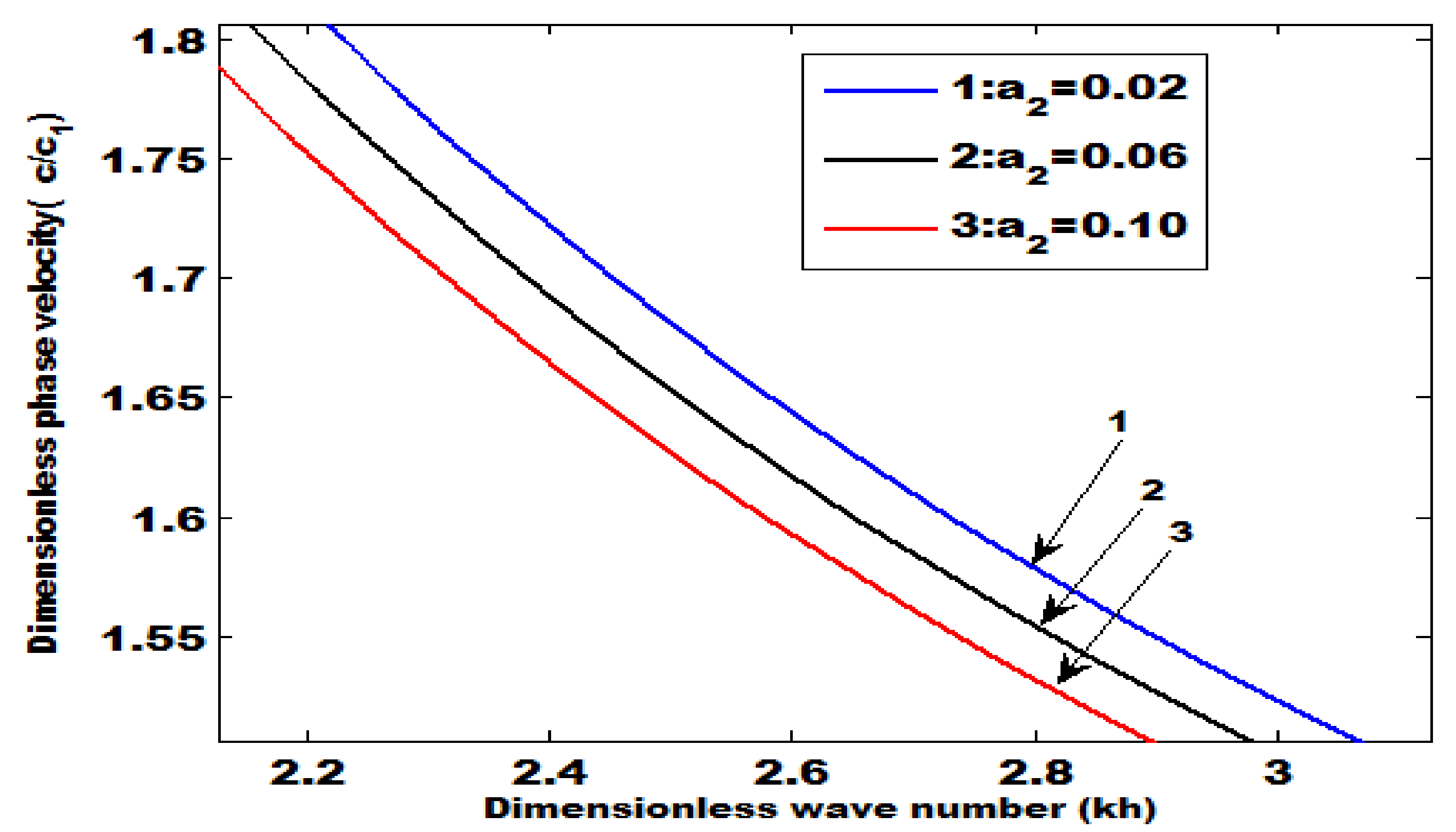
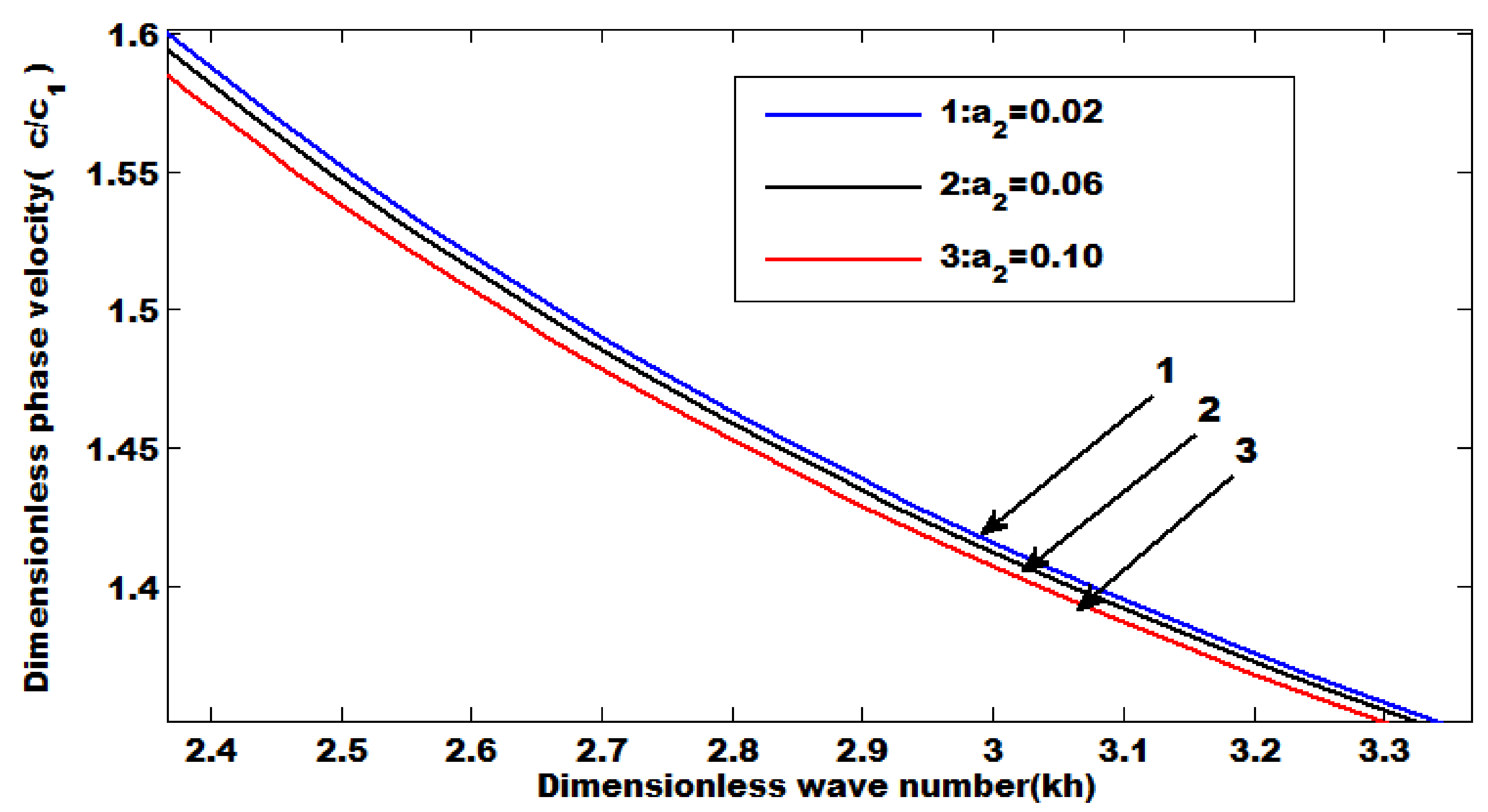
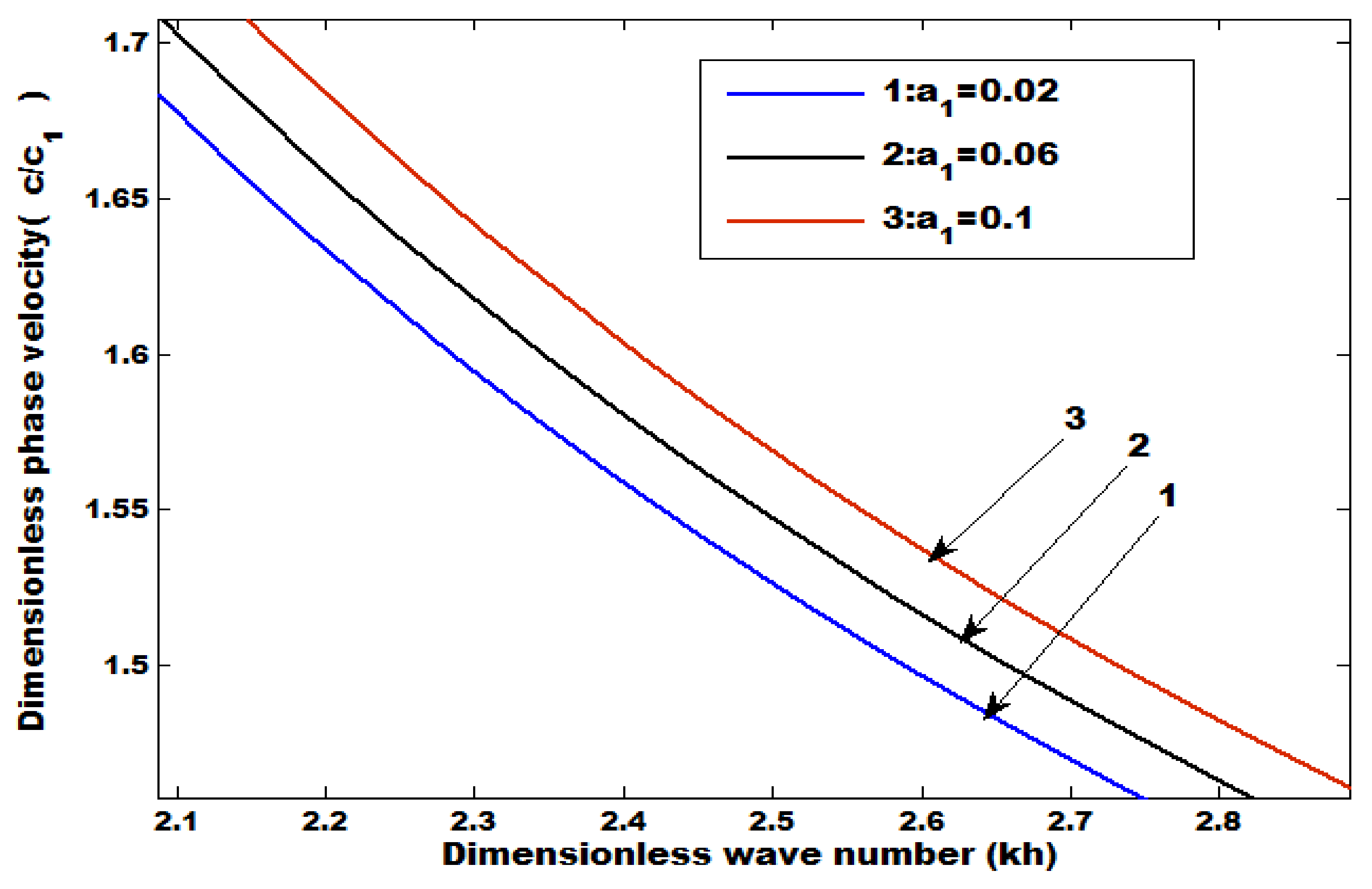
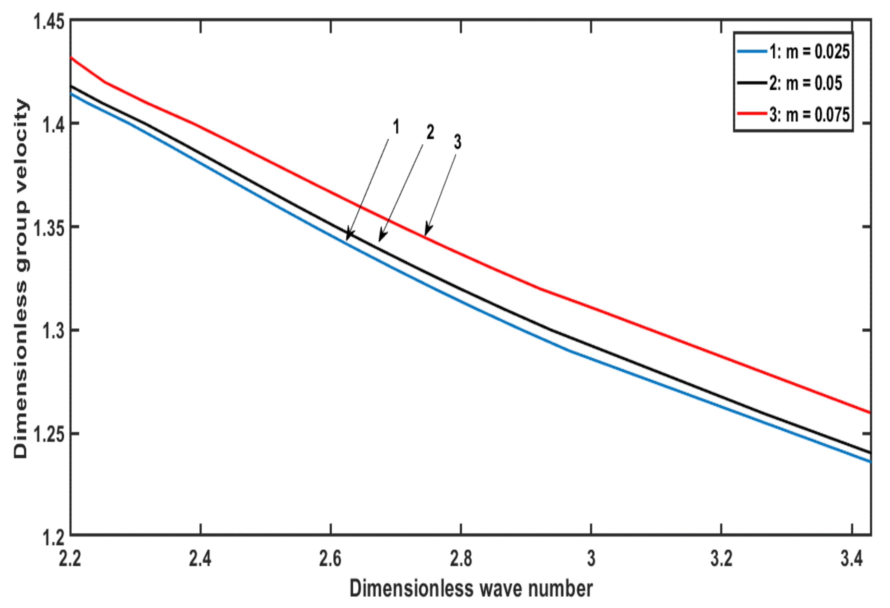
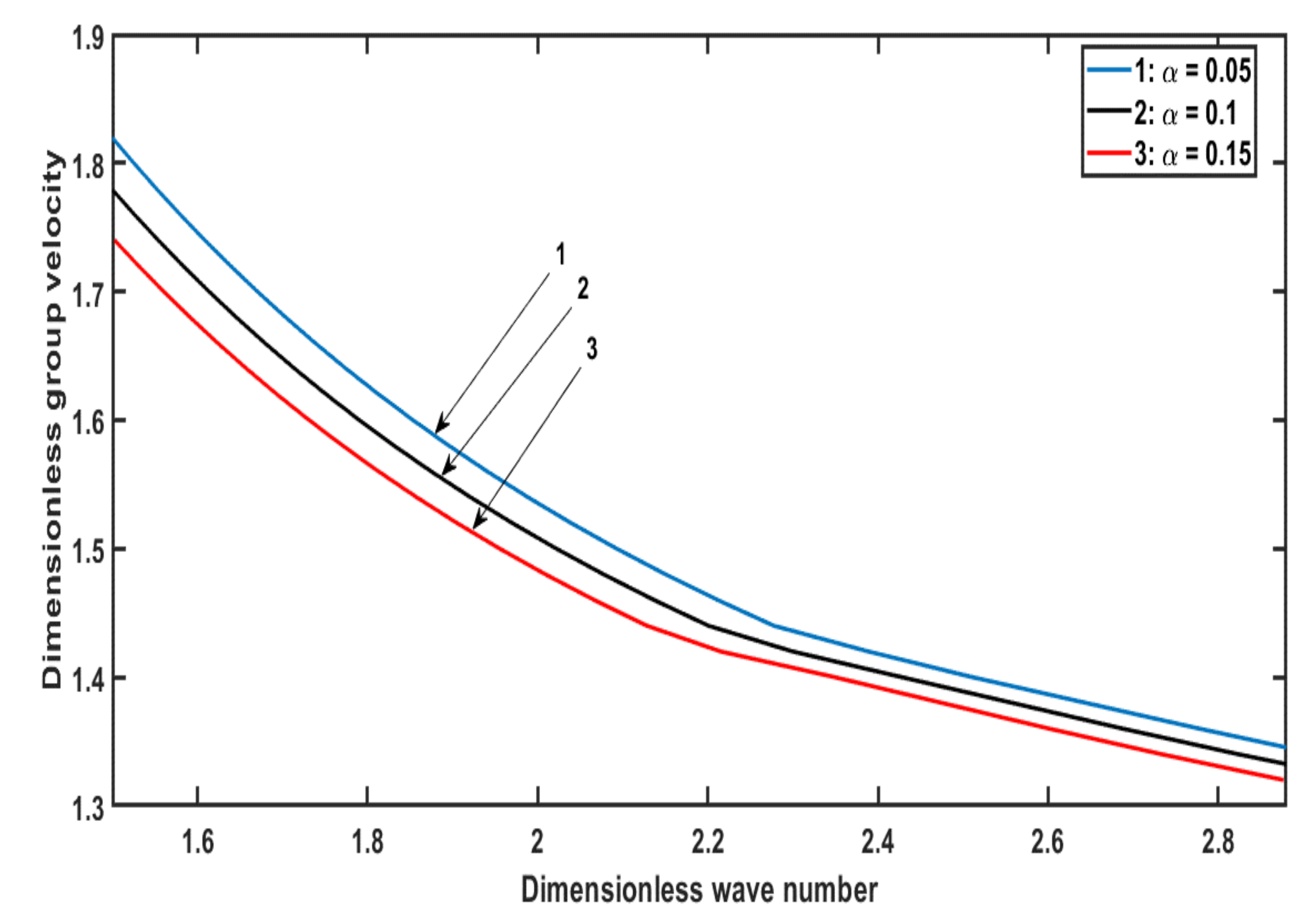
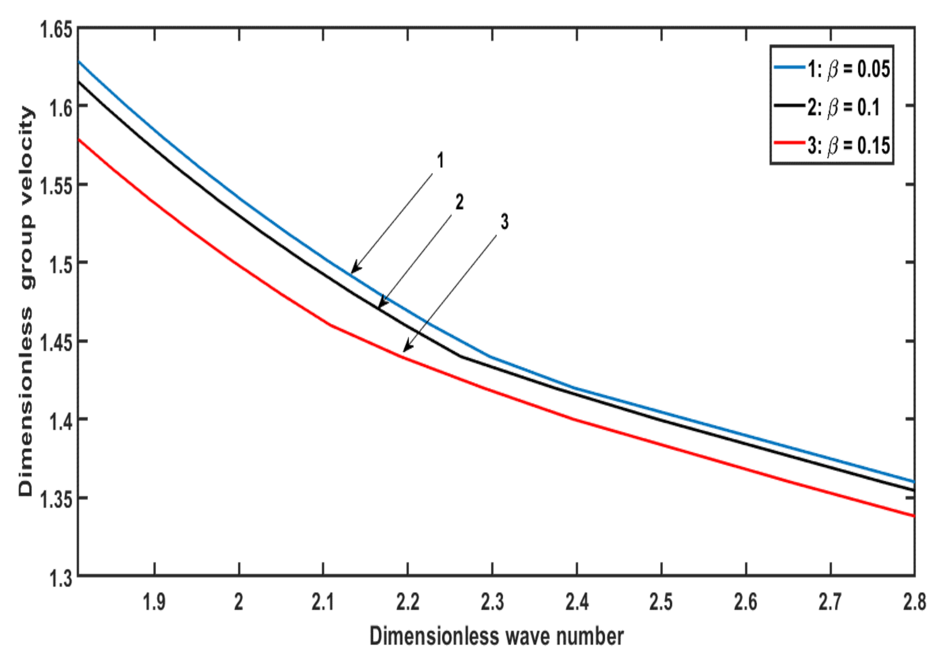
• An increase in the coupling parameter and position parameter increases the phase velocity.
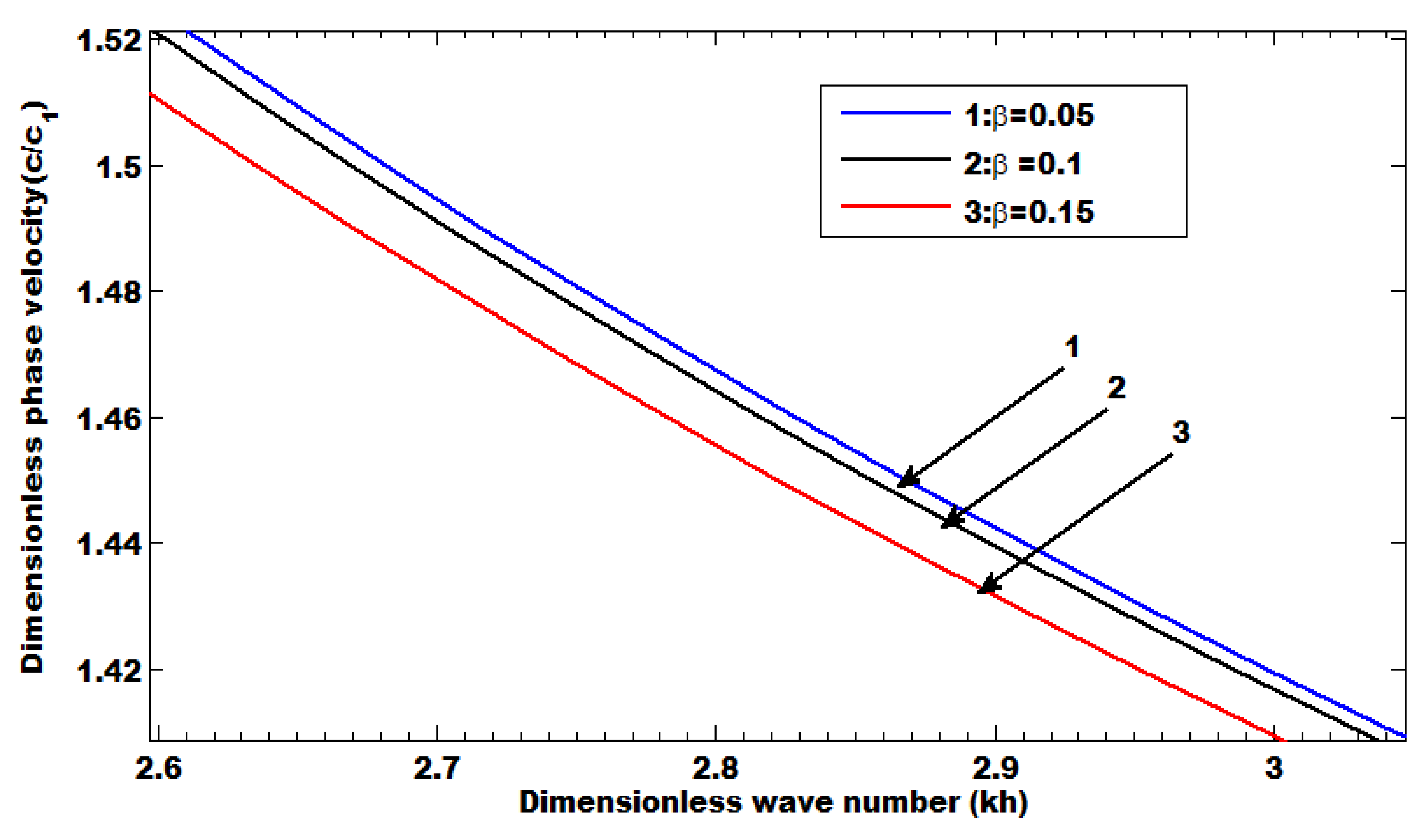
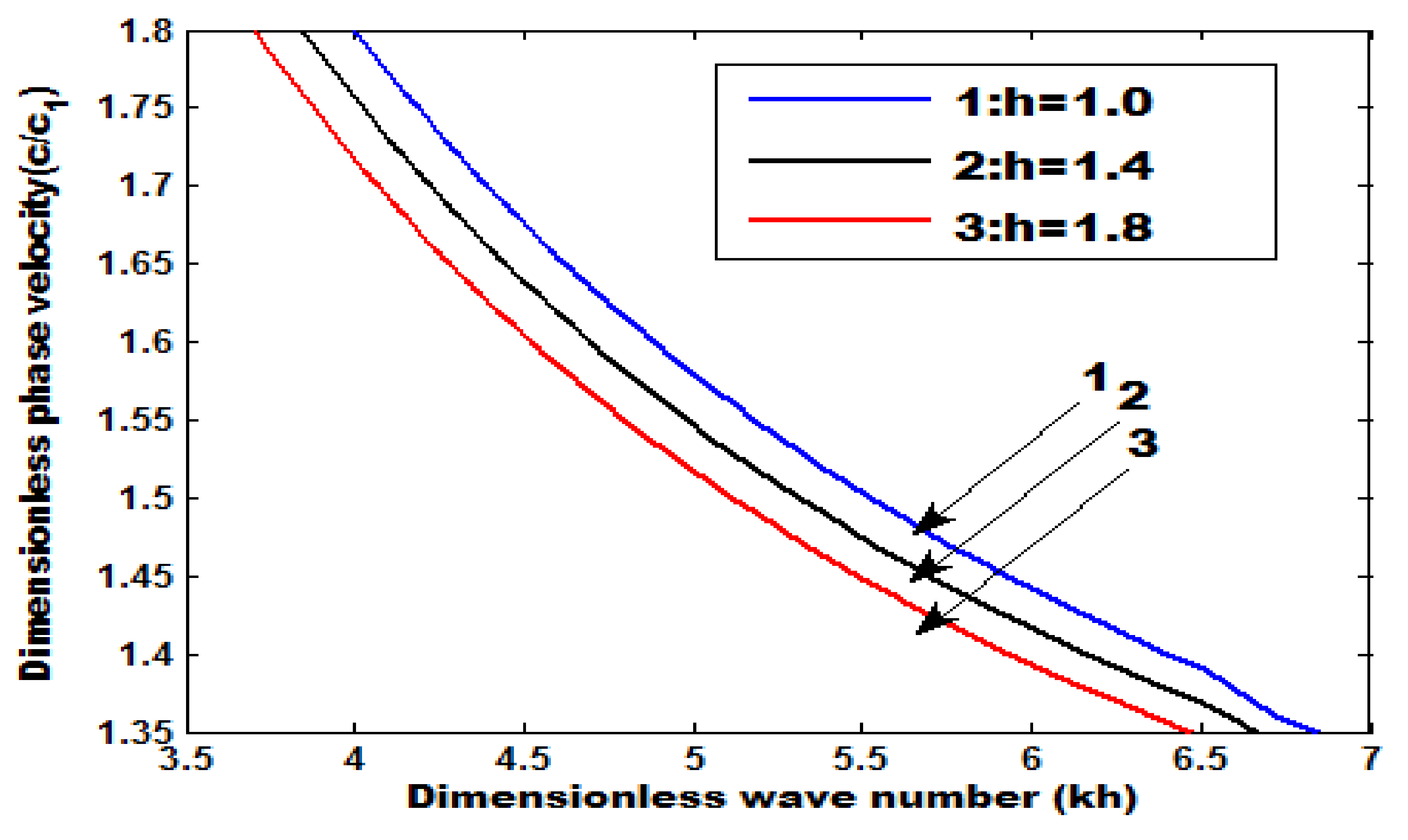
• The phase velocity decreases by increasing the heterogeneous parameters.
• The magnitude of phase velocity is greater in the absence of a common surface compared with the absence of an upper free surface.

References

1. Jeffreys, H. The Effect on Love Waves of Heterogeneity in the Lower Layer. Geophys. J. Int. 1928, 2, 101–111. [Google Scholar] [CrossRef] [Green Version]
2. Bullen, K.E. The problem of the earth’s density variation. Bull. Seismol. Soc. Am. 1940, 30, 235–250. [Google Scholar] [CrossRef]
3. Wilson, J.T. Surface waves in a heterogeneous medium. Bull. Seismol. Soc. Am. 1942, 32, 297–304. [Google Scholar] [CrossRef]
4. Dhua, S.; Chattopadhyay, A. Wave propagation in heterogeneous layers of the Earth. Waves Random Complex Media 2016, 26, 626–641. [Google Scholar] [CrossRef]
5. Alam, P.; Kundu, S.; Gupta, S. Dispersion study of SH-wave propagation in an irregular magneto-elastic anisotropic crustal layer over an irregular heterogeneous half-space. J. King Saud Univ.–Sci. 2018, 30, 301–310. [Google Scholar] [CrossRef]
6. Khan, A.A.; Umar, A.; Zaman, A. Rayleigh waves propagation in anisotropic layer superimposed a monoclinic medium. Indian J. Phys. 2019, 95, 449–457. [Google Scholar] [CrossRef]
7. Ilyashenko, A.V.; Kuznetsov, S.V. SH waves in anisotropic (monoclinic) media Z. Angew. Math. Phys. 2018, 17, 69. [Google Scholar] [CrossRef]
8. Singh, B.; Yadav, A.K. Plane wave in a rotating monoclinic magneto-thermoelastic medium. J. Eng. Phys. Phys. 2016, 89, 1393–1399. [Google Scholar]
9. Kumar, S.; Pal, P.C.; Majhi, S. Reflection and transmission of plane SH-waves through an anisotropic magnetoelastic layer sandwiched between two semi-infinite inhomogeneous viscoelastic half-spaces. Pure Appl. Geophy. 2015, 172, 2621–2634. [Google Scholar] [CrossRef]
10. Zhang, Y.; Xu, G.; Zheng, Z. Terahertz waves propagation in an inhomogeneous plasma layer using the improved scattering-matrix method. Waves Random Complex Media 2020, 1–15. [Google Scholar] [CrossRef]
11. Rao, Q.; Xu, G.; Wang, P.; Zheng, Z. Study on the Propagation Characteristics of Terahertz Waves in Dusty Plasma with a Ceramic Substrate by the Scattering Matrix Method. Sensors 2021, 21, 263. [Google Scholar] [CrossRef] [PubMed]
12. Rao, Q.; Xu, G.; Wang, P.; Zheng, Z. Study of the Propagation Characteristics of Terahertz Waves in a Collisional and Inhomogeneous Dusty Plasma with a Ceramic Substrate and Oblique Angle of Incidence. Int. J. Antennas Propag. 2021, 2021, 6625530. [Google Scholar] [CrossRef]
13. Biot, M.A. The Influence of Initial Stress on Elastic Waves. J. Appl. Phys. 1940, 11, 522–530. [Google Scholar] [CrossRef]
14. Chatterjee, M.; Dhua, S.; Chattopadhyay, A.; Sahu, S.A. Reflection and Refraction for Three-Dimensional Plane Waves at the Interface between Distinct Anisotropic Half-Spaces under Initial Stresses. Int. J. Géoméch. 2016, 16, 04015099. [Google Scholar] [CrossRef]
15. Singh, A.K.; Das, A.; Parween, Z.; Chattopadahyay, A. Influence of initial stress, irregularity and heterogeneity on Love-type wave propagation in double pre-stressed irregular layers lying over a pre-stressed half-space. J. Earth Syst. Sci. 2015, 124, 1457–1474. [Google Scholar] [CrossRef] [Green Version]
16. Abd-Alla, A.M.; Abo-Dahab, S.M.; Kilany, A.A. SV-waves incidence at interface between solid-liquid media under electromagnetic field and initial stress in the context of three thermoelastic theories. J. Therm. Stresses 2016, 39, 960–976. [Google Scholar] [CrossRef]
17. Verma, A.K.; Chattopadhyay, A.; Singh, A.K. Influence of Heterogeneity and Initial Stress on the Propagation of Rayleigh-type Wave in a Transversely Isotropic Layer. Procedia Eng. 2017, 173, 988–995. [Google Scholar] [CrossRef]
18. Khan, A.A.; Afzal, A. Influence of initial stress and gravity on refraction and reflection of SV wave at interface between two viscoelastic liquid under three thermoelastic theories. J. Braz. Soc. Mech. Sci. Eng. 2018, 40, 208. [Google Scholar] [CrossRef]
19. Tomar, S.K.; Kaur, J. Shear waves at a corrugated interface between anisotropic elastic and visco-elastic solid half-spaces. J. Seism. 2007, 11, 235–258. [Google Scholar] [CrossRef]
20. Whittaker, E.; Watson, G.N. A Course of Modern Analysis; Universal Book Stall: New Delhi, India, 1990. [Google Scholar]
21. Gubbin, D. Seismology and Plate Tectonics; Cambridge University Press: Cambridge, UK, 1990. [Google Scholar]
Figure 1. The phase velocity with wave number when   a 1 = 0.1 ,   α = 0.2 ,   β = 0.1 ,   h = 0.04 ,   p = 0.01 ,   a 2 = 0.2 .
Mathematics 09 03243 g001
Figure 2. The phase velocity with wave number when a 1 = 0.1 ,   p = 0.01 ,   a 2 = 0.2 ,   m = 0.08 ,   h = 0.04 ,   α = 0.2 .
Mathematics 09 03243 g002
Figure 3. The phase velocity with wave number when a 1 = 0.1 ,   p = 0.01 ,   a 2 = 0.2 ,   h = 0.04 ,   m = 0.08 ,   β = 0.1 .
Mathematics 09 03243 g003
Figure 4. The phase velocity with wave number when a 1 = 0.1 ,   β = 0.1 ,   h = 0.04 ,   a 2 = 0.2 ,   m = 0.08 ,   α = 0.2 .
Mathematics 09 03243 g004
Figure 5. The phase velocity with wave number when m = 0.08 ,   a 1 = 0.1 ,   p = 0.01 ,   a 2 = 0.2 ,   α = 0.2 ,   β = 0.1 .
Mathematics 09 03243 g005
Figure 6. The phase velocity with wave number when a 1 = 0.1 ,   m = 0.08 ,   h = 0.04 ,   p = 0.01 ,   α = 0.2 ,   β = 0.1 .
Mathematics 09 03243 g006
Figure 7. The phase velocity with wave number when a 1 = 0 ,   m = 0.08 ,   h = 0.04 ,   p = 0.01 ,   α = 0.2 ,   β = 0.1 .
Mathematics 09 03243 g007
Figure 8. The phase velocity with wave number when m = 0.08 ,   a 2 = 0.2 ,   h = 0.04 ,   p = 0.01 ,   α = 0.2 ,   β = 0.1 .
Mathematics 09 03243 g008
Figure 9. The phase velocity with wave number when m = 0.08 ,   a 2 = 0 ,   h = 0.04 ,   p = 0.01 ,   α = 0.2 ,   β = 0.1 .
Mathematics 09 03243 g009
Figure 10. The group velocity with wave number when a 1 = 0.1 ,   p = 0.01 ,   a 2 = 0.2 ,   h = 0.01 ,   α = 0.2 ,   β = 0.1 .
Mathematics 09 03243 g010
Figure 11. The group velocity with wave number when a 1 = 0.1 ,   p = 0.01 ,   m = 0.08 ,   h = 0.04 ,   a 2 = 0.2 ,   β = 0.1 .
Mathematics 09 03243 g011
Figure 12. The group velocity with wave number when a 1 = 0.1 ,   p = 0.01 ,   m = 0.08 ,   a 2 = 0.2 ,   α = 0.2 ,   h = 0.04 .
Mathematics 09 03243 g012
Publisher’s Note: MDPI stays neutral with regard to jurisdictional claims in published maps and institutional affiliations.